Autonomous Data Collection Techniques for
Approximating Marine Vehicle Kinematics
by
Jacob Gerlach
B.S. Naval Architecture, United States Naval Academy (2008)
Submitted to the Department of Mechanical Engineering
in partial fulfillment of the requirements for the degrees of
~~uJ C=:> U-1 ci_:
w
I
Master of Science in Naval Architecture and Marine Engineering
and
Master of Science in Ocean Engineering
at the
MASSACHUSETTS INSTITUTE OF TECHNOLOGY
June 2015
Massachusetts Institute of Technology 2015. All rights reserved.
A uthor ...
Certified by...
Signature redacted
Departrfmnt of Mechanical Engineering
May 8, 2015
Signature redacted
Michael R. Benjamin
Research Scientist, Department of Mechanical Engineering
Certified by...
A 1,1' , Thesis
supervisor
Signature redacted
....
/
John. J>Leonard
Samuel C. Collins Professor of Meclaf cal and Ocea Engineering
-"
/esi
8'uervisorAccepted by
...
Signature redacted
...
David E. Hardt
Chairman, Department Committee on Graduate Students
Autonomous Data Collection Techniques for Approximating
Marine Vehicle Kinematics
by
Jacob Gerlach
Submitted to the Department of Mechanical Engineering on May 8, 2015, in partial fulfillment of the
requirements for the degrees of
Master of Science in Naval Architecture and Marine Engineering and
Master of Science in Ocean Engineering
Abstract
Understanding vehicle kinematics is essential in allowing autonomous guidance al-gorithms to accurately assess short range encounters. Low cost, reconfigurable au-tonomous vehicles motivate using in-field online techniques rather than tow tank test-ing or Computational Fluid Dynamics (CFD). While the parameters of many physical dynamic models can be obtained using System Identification (SI) techniques, these models require knowledge of the vehicle actuators, which may not be the case in a "backseat driver" architecture using payload autonomy. Even when an identified physical model is available, using it to simulate trajectories requires insight into the design of the relevant controller, which may be proprietary or otherwise unknown to the back seat. This thesis develops a data collection procedure to obtain empiri-cal kinematic trajectories for unmanned surface vehicles (USVs). A linear black box model of the USV yaw system is also developed, using only data available in the backseat. A prediction table for the M200 USV is developed with both techniques.
Thesis Supervisor: Michael R. Benjamin
Title: Research Scientist, Department of Mechanical Engineering
Thesis Supervisor: John. J. Leonard
Acknowledgments
First, thanks to my parents for fostering a love for education and an insatiable cu-riosity about the world. All of my success can probably be traced back to a mother that read to me.
I am indebted to the Navy for offering me the fantastic opportunity to go to MIT
as my job. I look forward to contributing to the Navy with everything I've learned here.
Thanks also to Alon Yaari. His efforts to develop and improve the MOOS interface to the M200's, maintenance of the vehicles themselves, and insights into their inner
workings were essential.
Thanks to John Leonard for his insight and valuable perspective on the greater world of robotics. I regret not getting his input earlier and more often.
This thesis would have been impossible without Kyle Woerner. I only became aware of MOOS-IvP through his promotion of course 2.680. Although highly chal-lenging, it was extraordinarily rewarding and I can't overstate how much I learned. His accompanying doctoral work was essential to this work. He was always quick to address mutual concerns, listen to ideas, and provide valuable advice.
A heartfelt thanks to Mike Benjamin. It's hard for me to imagine how much better
my education over the years would have been if every teacher invested as much time and personal interest in their students.
I can't offer enough thanks to my wife Monica and sons Noah and Elijah. My
family was always patient with long hours, late nights, and coding on the couch. Without their support, I could never have finished this work.
Contents
1 Introduction 1.1 Motivation. . . . . 1.2 Overview. . . . . 2 Background 2.1 Guidance ... ... 2.1.1 Path Planning . . . . 2.1.2 Path Smoothing . . . .2.1.3 Short Range Avoidance . . . . 2.2 Dynamics and Control . . . . 2.2.1 Notation . . . . 2.2.2 System Models . . . .
2.2.3 On Line Identification . . . . 2.2.4 Control vs Trajectory Prediction . . . . .
2.3 Payload Autonomy . . . .
3 Approximate Vehicle Kinematics
3.1 Advance and Transfer . . . .
3.2 Kinematics Lookup Table . . . .
3.3 Measuring Kinematic Trajectories . . . .
3.3.1 Data Collection . . . .
3.3.2 Fitting, Approximation, and Interpolation 3.4 Black Box Modeling . . . .
13 13 14 15 . . . . 15 . . . . 15 . . . . 15 . . . . 17 . . . . 20 . . . . 21 . . . . 21 . . . . 22 . . . . 23 . . . . 23 27 . . . . 27 . . . . 29 . . . . 30 . . . . 30 . . . . 31 . . . . 31
3.4.1 Black Box Yaw System . . . . 31
3.4.2 Black Box Modeling of M200 Using In-Water Data . . . . 35
3.4.3 Model Improvements . . . . 37
3.5 Sum m ary . . . . 39
4 MOOS Applications and Behaviors 41 4.1 MOOS-IvP . . . . 41
4.2 TurnSequence Class . . . . 42
4.3 pDynamicsMonitor . . . . 43
4.4 Behaviors . . . . 43
4.4.1 ConditionSet . . . . 44
4.4.2 Operating Region and Container . . . . 44
4.4.3 Constant Heading and Speed . . . . 45
4.5 AVK Collection Mission . . . . 46
4.6 Summary . . . . 49
5 Experimental AVK Results 51 5.1 Results from Experimental Simulations . . . . 51
5.2 In-Water Observed Characteristics . . . . 53
5.3 Sum m ary . . . . 56
6 Future Work 61 6.1 Utility of AVK . . . . 61
6.2 Vehicle State . . . . 61
6.3 Dealing with External Forces . . . . 63
7 Conclusions 65
List of Figures
2-1 Short range avoidance of second obstacle . . . . 18
2-2 Using buffers to compensate for unknown kinematics . . . . 19
2-3 Infeasibility of course reversal . . . . 20
3-1 Advance and Transfer . . . . 28
3-2 USV yaw motion as a System . . . . 32
3-3 Black Box model of USV yaw System . . . . 33
3-4 Kingfisher M200 . . . . 35
3-5 Parameter Identification with M200 data . . . . 37
3-6 Parameter Identification with M200 data . . . . 38
3-7 Black Box Trajectory Prediction . . . . 39
3-8 Black Box Trajectory Prediction . . . . 40
3-9 Influence of History in Black Box Model . . . . 40
4-1 Basic Mission Simulation . . . . 48
AppTick influence on simulation consistency . . Variation in simulation results . . . . Variation in experimentally observed trajectories Experimental M200 Advance Characteristics Experimental M200 Transfer Characteristics Developing mean turn from experimental data Comparison of Predictions of 70 degree turn . Comparison of Turn Prediction Techniques . . . on the M200 . . . . 53 54 . . . . 54 . . . . 55 . . . . 56 . . . . 57 . . . . 58 . . . . 59 5-1 5-2 5-3 5-4 5-5 5-6 5-7 5-8
A-1 M200 Summary Data ... . 68
A-2 M200 Summary Data ... . 69
A-3 M200 Summary Data ... . 70
A-4 M200 Summary Data ... . 71
A-5 M200 Summary Data, Outliers removed ... ... 72
A-6 Comparison of Turn Prediction Techniques . . . . 73
List of Tables
2.1 6-DOF Dynamic and Kinematic Notation ... 21
3.1 Key M200 configuration parameters . . . . 35
5.1 Key simulation configuration parameters . . . . 52
Chapter 1
Introduction
1.1
Motivation
As Autonomous Marine Vehicle (AMV) technology proliferates, there is an ever in-creasing demand for improving their performance. Improvements to endurance, sens-ing, and intelligence are actively researched and continuously implemented.
One of the core subsystems of any autonomous vehicle is Navigation, Guidance, and Control (NGC). The navigation component can be as simple as obtaining data from GPS for a simple USV or as complex as fusing information from a compass, in-ertial navigation system, and data from fathometers and acoustic positioning systems to maintain an accurate estimate of position for the duration of a UUV mission.
Vehicle guidance consists of choosing the vehicle's course and speed. Often, the vehicle's path for an entire mission or portion of a mission is determined at once, a process called path planning in the literature. Guidance functions may also in-clude reactive components, either determining the desired heading instantaneously or modifying a pre-planned path when new information is obtained.
With the vehicle's trajectory determined by the guidance component, the vehicle control system must determine how to command the vehicle's actuators in order to achieve the desired course and speed. Most AMV's are underactuated and nonholo-nomic and research into various control methodologies remains highly active.
opera-tors, and the optimal solution varies based on the desired budget, capabilities, and flexibility. One gap in the existing options is the capability to provide accurate ve-hicle guidance for short range encounters on low cost veve-hicles using an architecture known as payload autonomy. The goal of this thesis is to develop data collection techniques needed to enable guidance algorithms operating in payload autonomy sys-tems to improve short range decision making by considering approximations of vehicle kinematics.
1.2
Overview
Chapter 2 reviews existing guidance and control methodologies and addresses why a new approach is pursued for payload autonomy. Chapter 3 describes a system to provide short term predictions of vehicle kinematics using either explicitly measured trajectories or a black box system model. The primary product of this thesis is software developed for MOOS-IvP, a modular, behavior based autonomy system. MOOS-IvP is described in Chapter 4 as are the algorithms and data collection mission developed in this work to collect kinematic data. Chapter 5 describes the validation of the data collection mission in simulation and on Kingfisher M200 USV's. Finally, Chapter 6 discusses some limitations of the current implementation and potential approaches to improve on these limitations.
Chapter 2
Background
2.1
Guidance
2.1.1
Path Planning
Path planning has its roots in early land based robots. Given a starting position, goal position, and some knowledge about obstacles, the robot must select a path to travel. Choosing a path is an optimization problem. The most obvious criterion to optimize is distance: what is the path that gets to the goal, avoiding the obstacles, while traveling the least distance? [12]
The basic problem formulation translates well to marine autonomy. The guidance component of many AMV missions can be framed as choosing or following a path while avoiding obstacles. Obstacle avoidance for other moving vessels imposes ad-ditional constraints on path planners, especially when there are protocols the AMV should respect. Woerner
[18]
discusses a variety of reasons to pursue AMV guidance approaches that incorporate the collision avoidance regulations (COLREGS) used by human steered ships [9].2.1.2
Path Smoothing
Depending on the path planning method used, the resulting optimum path may be piecewise linear. For underactuated vehicles, a piecewise linear path cannot be
accu-rately followed. Various approaches exist in the literature to generate smooth paths. The simplest approach is to generate a smooth path that passes through the way-points determined by a simple path planning algorithm. This approach is generally implemented by smoothing after a path has been selected rather than being part of the optimization process [8].
One simple smoothing method is the cubic spline. It is straightforward to fit a cubic spline through path planner waypoints. This guarantees that the curvature of the path is continuous, which is an improvement. Cubic splines suffer from the fact that the entire path is affected by each waypoint. This may mean that the smoothed path may be significantly different from the path originally determined by the planner, potentially sacrificing optimality or even being unsafe. It also means that the entire path must be recalculated if a local modification is performed (say, for obstacle avoidance). Finally, although the cubic spline path has a continuous second derivative, it is not necessarily dynamically feasible. [8]
One alternative to cubic splines is B splines. B-splines have an advantage over cubic splines because each control point only has local influence. Moving a control point, for example to conduct local path modifications, only modifies a portion of the path. Despite this advantage, B splines still do not explicitly account for the maneuvering characteristics of the vehicle. However, one guidance algorithm can dynamically change the order of a B-spline used to smooth the path between planned waypoints [13]. Higher order splines were found to be tracked more easily by the vehicle.
Rather than modifying a path to make it smooth, many path planning algorithms explicitly consider a dynamic constraint as part of the planning algorithm. For ex-ample, some path planning approaches include curved segments with limited radius of curvature, accounting for the vehicle's turning capability [15]. This simplifies the vehicle's turning kinematics to a combination of straight line motion and constant
radius of curvature turns. While turning radius is an important constraint, it can only represent the kinematics of a vehicle that has achieved a steady state turn.
dy-namically feasible paths, their application in the literature is limited to cases where standoff ranges to obstacles are sufficient that the transition from straight travel to steady state turning is not significant.
2.1.3
Short Range Avoidance
In general, good seamanship (in practice) and the Collision Regulations'
191
(bystatute) dictate that avoidance maneuvers be taken early and should result in comfort-able passing distances rather than more "efficient" maneuvers which might narrowly avoid collision. Nevertheless, there are cases where understanding the limits of the vehicle's maneuvering capabilities is necessary to take appropriate action. While the notion of "short" range depends in general on vehicle size, it depends more specifically on the vehicle's maneuvering characteristics. There is no precise definition for short range, but several cases are presented where range to obstacles is on the order of the
vehicle's turning radius. These cases certainly qualify as short range.
Formation control for multiple cooperating AMVs is an active area of research. Depending on the application, it may be desirable to maintain very short ranges between members of the swarm.
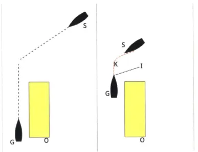
In some complex interactions, it may be necessary to delay taking avoidance action because of a second obstacle. Figure 2-1 depicts one such possibility. In this and other cases, must know their maneuvering capabilities to determine the correct maneuver.
Guidance algorithms that seek to employ COLREGS protocols for vessel interac-tions must handle situainterac-tions where course and speed are constrained as the "stand on" vessel2. If the other vessel, required to "give way"3, does not take appropriate action,
the stand on vessel may have the option (Rule 17.a.ii) or obligation (Rule 17.b) to take avoidance action at short range. As in Figure 2-1, the correct maneuver in any given situation may depend on the maneuverability of the vessel in question.
Finally, autonomous sensing and classification of obstacles still has significant 'See Rule 8.
2
See Rule 17.
4
G
G 0
Figure 2-1: Motivation for Short Range Avoidance: Remaining to the left of obstacle 0 means that vessel G is unable to maneuver to avoid vessel S until close range. G's maneuvering capabilities may make it impossible to keep clear of S while turning (path K), in which case she should slow and allow S to pass ahead rather than maintaining speed and trying to maneuver. Assuming an instantaneous turn (path I) will incorrectly make a collision free turn appear feasible
challenges. Advances in radar, LIDAR, and stereo vision are enhancing sensing capa-bility, and methods to fuse data from multiple sensors are improving. Nevertheless, delays in sensing obstacles may require an AMV to take avoidance action at short range.
While research into techniques such as model predictive control is ongoing and practical implementations are used on some aircraft, most algorithms employed in currently fielded AMVs do not consider the kinematics associated with the initiation of a turn. As underactuated vehicles, any AMV with an initial forward speed will have some "advance4" in the original direction of travel while turning to a new course. In one autonomy system, obstacle and contact avoidance behaviors consider a straight line from the vehicle's position to the obstacle
[4].
Candidate courses are evaluated based on the CPA resulting from this straight line, effectively assuming that the vehicle can make instantaneous turns. A similar approach uses behavior voting for candidate trajectories - arcs laid out such that each cell in a grid is covered[11]. In both of these cases, the evaluation criteria do not consider the advance required to4The term "advance" refers to translation in the original direction of motion during a turn. Advance and its counterpart transfer are discussed in more detail in Section 3.1.
achieve the new course.
These approaches and others currently in use benefit from the fact that obstacles and collision avoidance standoff ranges are typically much larger than the advance distance associated with a particular course change. Furthermore, the NGC system updates decisions and control action many times while approaching such an obstacle.
A small error in estimation of the vehicle's trajectory can typically be compensated
for with future guidance and control decisions.
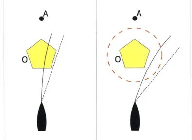
Consider, however, an obstacle detected at close range, as shown in Figure 2-2. Without knowledge of the expected vehicle kinematic trajectory, the first course would be selected and a collision could occur. Buffer zones around obstacles help compensate for this, but this is limiting in a crowded obstacle field such as a minefield. Buffers would also be inadequate to enable accurate navigation in a narrow channel.
A A
0 0
Figure 2-2: Inadequacy of assuming Instantaneous Turns: A vehicle driving to waypoint A must avoid obstacle 0. At close range, collision may occur due to the difference between an instantaneous turn and actual vehicle trajectory. If an offset is added to the obstacle, a larger turn is executed and collision is avoided.
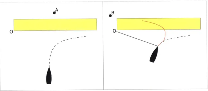
Alternatively, consider the scenario shown in Figure 2-3. Assuming instantaneous turn capability results in an inaccurate expectation of reversing course to pass to the opposite side of an obstacle. This type of difficulty was encountered in [11], which describes an issue with decision making fluctuating between alternate sides of an obstascle. Similar issues have occurred in obstacle avoidance algorithms in the
MOOS-IvP autonomy software used in this thesis. In both cases, a sort of decision making hysteresis was introduced to "commit" to passing on one side of an obstacle. An algorithm that considers the expected vehicle kinematics would inherently recognize the impossibility of immediately changing course to cross to the other side and would make the correct decision without artificial coping mechanisms.
0B
0 0
Figure 2-3: Motivation for Short Range Avoidance: Initially, the vehicle has decided to pass to the right of obstacle 0 to reach waypoint A. Later, some other factor has updated the waypoint to B and passing to the left of the obstacle is preferable. Assuming either instantaneous course change or instantaneously achieving a maximum turn rate makes this option appear possible. In reality, the vehicle cannot reverse course without colliding with the obstacle.
Given these types of challenges, it is clear that guidance algorithms cannot be assured of taking the right action in short range engagements without knowledge of
the turning kinematics.
2.2
Dynamics and Control
Models of vehicle dynamics have been used extensively in the field of control theory.
If the necessary parameters are known, the equations of motion can be used directly
to solve for the vehicle's motion based on the applied forces. This leads directly to a prediction of the vehicle's kinematics for a given force input. This type of kinematic prediction would be suitable for enhancing guidance algorithms to better handle short range encounters.
2.2.1
Notation
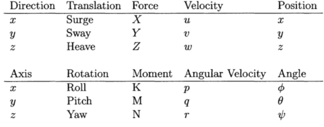
Notation in this this thesis follows the conventions given in [10], summarized in Table 2.1. Additionally, AO is used to denote the discrete heading change associated with a specific intended turn.
Table 2.1: Summary of notation used for kinematics and dynamics in six degrees of freedom. Direction Translation Force Velocity Position
x Surge X u x
y Sway Y v y
z Heave Z w z
Axis Rotation Moment Angular Velocity Angle
x Roll K p
y Pitch M q 6
z Yaw N r
2.2.2
System Models
The 6 DOF motion of a marine vehicle on the surface (such as a USV) is usually simplified to plane motion for steering models, neglecting the influence of roll, pitch, and heave. With these simplifications, both linear and nonlinear approaches exist to
treat the motion of the vehicle with varying degrees of accuracy. After simplifying to
3-DOF the equation of motion is given [101 by
Mu + D(u)u = f(u) (2.1)
u = [u, v, r]T is the planar velocity, M is the inertia matrix (including added mass),
and D is the hydrodynamic drag matrix. f(u) is the vector of forces on the vehicle, including actuators and environmental forces. This model might prove inadequate
when substantial pitch and roll motions occur (in heavy seas, for example), but is
sufficient for many situations where out of plane motions are not significant.
in M and D gives a planar model for vehicle dynamics
m1 1it - m22vr + diu = f
m22i + 'mur
+
d2v = 0 (2.2)m3 3r + mldUV + d3r = T
While some applications may require models with less assumptions and simplifications (for example, including external forces), it has been noted that the majority of USV heading controllers are based on this model [2].
Determining the added mass and hydrodynamic drag coefficients in M and D is a form of system identification (SI). Traditionally, SI for a large ship would be performed experimentally. Computational Fluid Dynamics is also capable of estimating the requisite coefficients. Both of these approaches can be expensive. A complete set of
SI experiments requires extensive time in a tow tank [1]. Commercial CFD software,
as an alternative, is itself costly and can require specialized computing hardware. Research and other activities are increasingly relying on larger numbers of small low cost AMVs. In this environment, it may not always be realistic to expect this type of analysis to be done. Furthermore, mission specific payloads have the potential to significantly change the identified properties. This could be as simple as changing the mass and displacement of the vehicle or could be more complex if the payload includes some type of sensor in the water [14]. SI, however performed, would have to be repeated for each configuration of the vehicle.
2.2.3
On Line Identification
An alternative to tow tank experiments and CFD is "on-line" system identification. This allows determining approximate hydrodynamic properties in the course of op-erating the vehicle in the real world. The flexibility afforded by this technique is an attractive solution when low cost vehicles and mission reconfigurability make it impractical to utilize other SI techniques.
will require some knowledge of the vehicle's actuators: rudder angle, propeller speed, etc. Depending on the type of model used, SI may also require measurements such as sway velocity. This follows from the idea of parameter identifiability
13].
This will become significant in Section 2.3 where sufficient measurements required to ensure system identifiability may not always be available.2.2.4
Control vs Trajectory Prediction
The typical use for dynamic models is in vehicle control -determining desired actuator motion to achieve a guidance objective. As discussed in Section 2.1.3, considering the turning kinematics in higher level control functions on AMVs is primarily necessary for short term path planning, typically in support of obstacle or collision avoidance. These objectives require predicting the vehicle's trajectory based on future control action. By predicting trajectories, guidance algorithms can be restricted to consider only dynamically feasible paths. Additionally, by more accurately understanding the expected kinematics associated with a given decision, algorithms can more effectively determine if that decision will actually achieve the intended objectives.
Given a dynamic model with the appropriate parameters identified, such a trajec-tory could be generated by simulating the actuator commands and resultant vehicle motion for a suitable guidance input. Note that this requires knowledge of both the physical properties of the vessel and also the design and parameters of the low level controller generating the actuator commands.
2.3
Payload Autonomy
Payload autonomy is an approach to autonomous vehicles that decouples high and low level control. A "front seat" vehicle computer handles low level control of the vehicle's actuators. The front seat controls actuators to achieve goals such as "desired heading" or "desired speed" that are requested by a separate autonomy "back seat". This has also been referred to as the "backseat driver design philosophy" [5].
agnostic to the hardware where it will be executed. This can provide logistical ad-vantages for organizations that deploy multiple different AMV's. Furthermore, an autonomy mission can be designed and implemented entirely on a payload computer. Provided with a payload interface, that mission should then be usable on any specific AMV. The notion of hardware agnostic payload autonomy imposes several limitations that make it challenging to allow the back seat autonomy system to use a dynamic system model for kinematic predictions.
The first challenge is limitations on the front to back seat interface. Increasing requirements beyond navigation data and simple goals like heading, depth, and speed complicates the interface. This is clearly not insurmountable, but leads to the next problem. Obtaining hardware independence means that a dynamics model in the backseat should work regardless of whether the autonomy mission is running on a differential drive catamaran or a monohull with a fixed propeller and rudder. This means that both the additional interfaces and the dynamics model used depend on the vehicle type.
Finally, even if the front to back seat interface were expanded to include all of the actuators and the dynamics model in the backseat where flexible enough to accom-modate all vehicle types, the front seat still has a controller that will influence the vehicle's kinematics. Predicting kinematics from the back seat would require modeling
not just the physical behavior of the vehicle, but also the behavior of the controller.
Model predictive control does exactly this (albeit without the restriction of payload autonomy). Work in [17] and
[16]
takes this approach, conducting path planning that explicitly models future control actions and vehicle dynamics to restrict path planning to dynamically feasible paths. While this is possible when the design of the control system is known, many commercial vehicles use proprietary controllers. An approach that approximates kinematics without requiring explicit knowledge of the controller is still desirable.This chapter has reviewed some existing techniques used to account for realistic vehicle kinematics in guidance algorithms, as well as approaches to rigorously account for the vehicle dynamics in control theory. The next chapter will describe a new
Chapter 3
Approximate Vehicle Kinematics
With the goal to provide platform independent short term prediction of turning kine-matics, a new approach is necessary. Given the limitations imposed by payload
auton-omy (Section 2.3), an empirical approach is warranted to provide broad applicability even when specific actuator movements are unknown. This means approximating the vehicle kinematics without the aid of a physical dynamic model (Section 2.2.2). Two alternatives are presented. First, in Section 3.3, an approach utilizing direct measure-ments of trajectories is described. This is approach is termed Approximate Vehicle Kinematics (AVK). An alternative approach, utilizing a black box model of the ship yaw system is described in section 3.4.
3.1
Advance and Transfer
Approximate kinematics have long held wide acceptance by human mariners. Coastal piloting has many of the same challenges described in Section 2.1.3. In general, over-lapping constraints require the ship's crew to execute very precisely timed maneuvers.
A prime example is maneuvering a large ship to remain within a channel. The
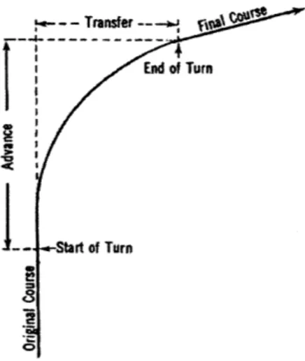
ve-hicle's kinematics are approximated by two linear distances: advance and transfer (Figure 3-1). These are defined as the distance traveled parallel and perpendicular to the vehicle's original course [7]. These distances are a function of vehicle speed u, initial rudder angle 60, and heading change AV):
(3.1)
Knowing these distances allows a ship's Navigator to conduct detailed advance planning for a turn, determining the exact point to initiate the turn ("Start of Turn" in Figure 3-1).
- Transfer -- SO t
End of Turn
--Start of Turn
Figure 3-1: Advance and Transfer as considered by typical navigation practice on ships. The helmsman deflects the rudder at the point labeled "Start of Turn". At some point during the turn, the helmsman shifts the rudder, and makes fine adjustments as necessary to steady the ship on the new heading. If the desired "End of Turn" point is known, the Advance and Transfer (known in advance for a given ship based on the intended speed and rudder angle) can be used to calculate the "Start of Turn" point. Image borrowed from [7].
Although advance and transfer are referenced to the rudder angle used to initiate the turn, 6(t) is not constant. The helmsman manipulates the rudder as appropriate to achieve the new course precisely ("End of Turn" on Figure 3-1). The expected rudder manipulation is implicit in the kinematic approximation. Furthermore, while the end of turn point is calculated, the trajectory between start and end is just an approximation made by drawing a fair line between the points [7].
Just as traditional navigation practice abstracts the actions of the helmsman, the payload autonomy approach abstracts the actions of the front seat controller. Where the goal of this technique in traditional navigation is essentially advance path planning (where exactly to execute a pre-planned maneuver), approximate kinematics are intended here to aid in evaluating the suitability of various maneuvers to achieve
reactive collision avoidance goals.
3.2
Kinematics Lookup Table
Just as advance and transfer for a large ship are functions of rudder angle, speed, and heading change (equation 3.1), the kinematic trajectory for a USV turn is a function of similar inputs. Where a ship's Navigator could direct differing amounts of rudder for one heading change, it is assumed here that the payload autonomy interface provides no provision for such a request. Therefore the actuator motions used to produce a certain heading change are assumed to be a single valued function of the guidance input and initial state:
[N(t), K(t)] = f(u, A0, r) (3.2)
where the yaw moment N(t) may be due to a rudder, differential propulsion, or some other method and the thrust K(t) may also change during a turn. Under this assumption, the vehicle's kinematics are then a function of initial state and turn parameters
x(t) f(X4, XO) (3.3)
where x =
[X,
y, b, v, r]. For the present work, consideration is restricted to initialstates xO where vo = ro = 0. This is a strong assumption and is discussed further in
Section 3.4 and Chapter 6.
In the absence of external influences such as current, the global position
[X,
y] and heading4
of the vehicle have no influence on the resulting trajectory. The turn trajectory can then be referenced to the body fixed reference frame P. fromthe moment the turn is initiated. JV has an origin [XN, YN] = [xO,o, yo,o] with the
positive y-axis oriented at Oo where (-)o represents the value at the start of the turn. The resulting trajectory starts at the origin of K, traveling initially in the positive y direction and is denoted
a left and right turn will be the same. Right turns are chosen to be the reference. For a given combination of (uo, AV), the corresponding left turn -AV) can be recovered
by reflecting the kinematic trajectory XN across the y axis of AP.
Under these assumptions, k = (uo, AO) with 0 < A@i K 180 uniquely identifies a
turn trajectory. As a practical matter, the space k can be discretized into appropriate intervals for data collection and vehicle planning. The discretization of k is referred to as a Cached Kinematics Table (CKT), where each cell in the table kij contains the trajectory x(t) associated with the turn (i = uo,
j
= AO). This structure fits verynaturally with a data collection mission and is consistent with the existing structure of the guidance decision space. Furthermore, the notion of caching this information may offer practical advantages for computational performance when used in guidance algorithms.
The specific discretization of the AVK table may vary. In a data collection mission, for example, it might be appropriate to choose a 20 degree A@ spacing to minimize the time associated with the mission. In guidance algorithms, on the other hand, it might be necessary to discretize to 1 degree to match the candidate headings being considered.
3.3
Measuring Kinematic Trajectories
3.3.1
Data Collection
In order to populate the table, each turn kij must be performed and the resulting trajectory recorded. This is achieved through a data collection mission, described in Section 4.5. Essential to this effort is controlling vehicle initial conditions and controlling the guidance input (i.e. keeping the desired heading constant).
One challenge in executing this mission is the presence of external influences such as wind and current. These have the potential to substantially influence vehicle turning characteristics. Accounting for these factors is complicated further on vehicles where the navigation system is not capable of determining both speed through the
water and speed over ground. Further discussion of possible techniques to exclude the influence of external forces is given in Section 6.3.
3.3.2
Fitting, Approximation, and Interpolation
An AVK trajectory collected in this manner is not directly useful. First, the position data recorded may be noisy. While the vehicle's speed generally changes during a turn, it is assumed here that the kinematic trajectory can be adequately approximated by assuming a constant speed during the turn, equal to the average speed required to traverse the recorded trajectory in the observed time. This assumption means that only the geometric shape of the input data needs to be retained, not the discrete time history. As a result, the input data can be simplified by approximating it with a function y = f(x) over an appropriate domain of x. Accompanying work to this thesis examines the suitability of various data fitting techniques. A fourth order polynomial was chosen, fit to the data using least squares regression.
To improve the computational efficiency of guidance algorithms using the AVK trajectory, the trajectory is further simplified by approximating the polynomial as a piecewise linear function.
Section 3.2 discussed possible discretizations of the CKT. If the experimentally collected data is sparse, trajectories in the table can be interpolated to provide data for cells in the fine discretization used for guidance.
3.4 Black Box Modeling
3.4.1
Black Box Yaw System
While AVK trajectories stored in a kinematics lookup table offer a significant im-provement in the predictive capability of a back seat guidance algorithm, the utility of the approach is severely limited by the restrictions on initial vehicle state intro-duced in Section 3.2. A system model, on the other hand, includes the current state explicitly and has fewer restrictions on applicability.
The physical dynamics models discussed in Section 2.2.2 predict vehicle motion on the basis of physical properties of the vehicle and its actuators. In the case of yaw dynamics, a simple example of this approach is the 1st-order Nomoto steering model
[101.
1 K
S= -- r + - (3.4)
T T
where J is the rudder angle and i is the derivative of yaw rate (i.e.
).
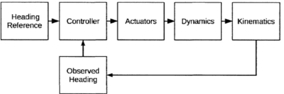
Some technique must be used to identify the parameters T (a time delay factor) and K (a proportionality constant for the effectiveness of the rudder). Once identified, this model (either in conjunction with a speed model or by assuming some speed profile) could be used to predict a vehicle's trajectory for some known rudder input 6(t) by simulating the system shown in Figure 3-2 (replacing the actual vehicle dynamics with the model).Heading Controller Actuators - Dynamics - Kinematics Reference
Observed Heading
Figure 3-2: The USV yaw motion as a system. The guidance component determines the heading reference. The navigation system provides feedback to the controller. In response to changes in the heading reference and feedback signal, the controller produces actuator motions. The actuators exert forces and moments on the vehicle, resulting in a certain kinematic profile depending on the inertial and hydrodynamic properties of the vehicle (i.e. the dynamics).
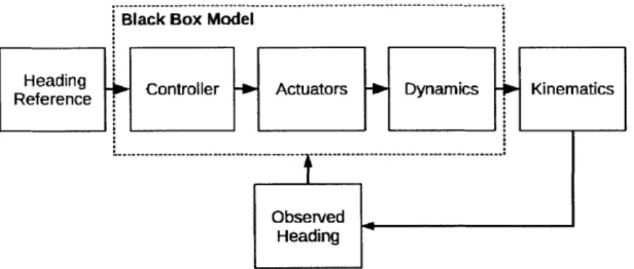
To avoid the need to simulate the controller and know actuator positions, a differ-ent model is considered. If the boundaries of the model are expanded to include both the control layer and the actuator dynamics, a black box model of the entire system is obtained as shown in Figure 3-3. The inputs are desired and observed headings and the output is vehicle's heading.
A simple linear model of this system is
Black Box Model
Re e Controller +ib Actuators -No Dynamics -i-Kinematics
Observed Heading
Figure 3-3: Black box model of USV yaw motion. The behavior of the controller and the actua-tors are modeled together with the vehicle dynamics. The resulting model can make a trajectory prediction without knowledge of the controller design or the actuator positions.
where E is a vector of the difference between the desired heading given by the heading
reference and the measured heading (Id - 0) at previous time steps. Similarly, / is
a vector of previous vehicle headings. Given a sample data set from the vehicle, a simple least squares fit of the parameters A and B serves to perform SI for the black box model.
It is noted that the choice of input data can have significant impact on the quality of the produced model. For example, if E and V) are monotonically increasing, then
A = 0 and B = [B1, 0, ... , 0] where B1 > 1 and the exact valuedepends on the input
data. Such a model is obviously inadequate and can never predict heading decreasing (i.e. left turns). An alternating set of left and right turns, like those shown in Figures
3-5 and 3-6 results in values for each element in A and B and can predict both right
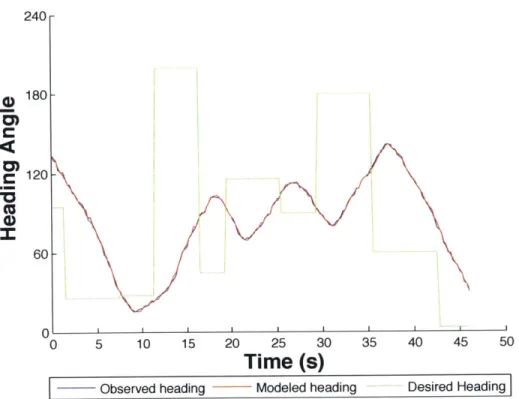
and left turns. Finally, it is noted in [10] that persistent excitation is preferred for system identification. This is addressed further in Section 3.4.2.
With A and B identified, the model can be used to predict turning trajectories
by simulating coordinates and heading changes.
" Begin with desired and actual heading for last n steps
" Construct error and heading vectors
" Use current x and y position, heading, and speed
- Given x, y, heading, and speed
- Estimate next x and y position from heading and speed
- From previous heading data, predict next heading using model
- From next heading, calculate e at next step
- Update error and heading vectors
A modeling approach has several advantages compared to the approach described
in Section 3.3. First, it nominally requires less data collection time. Rather than fully discretizing the kj domain with data collection points, an appropriate sequence of input data is collected at each speed.
A significant weakness that arises from the CKT structure and the direct
mea-surement AVK approach is that the stored turn trajectories can only be used to directly predict trajectories that match the vehicle's behavior during data collection (i.e. the conditions associated with a certain CKT cell). In the present work, this means the vehicle is on a steady course. Once the vehicle has started turning, the
trajectories stored in the table cannot accurately predict the vehicle's path. Despite
potential options to allow the CKT/AVK approach to more robustly handle varied vehicle initial conditions (Section 6.2), incorporating these changes into the system increases complexity and may also require changes to the data collection mission.
A system model, by nature of considering the system state and recent state history,
is able to generate a prediction anywhere along the trajectory of a turn. This avoids the need to classify the vehicle's current state (steady vs. turning) and have special cases to build a trajectory prediction accordingly.
Despite these advantages, obtaining an adequate model is not trivial. The model proposed in Equation 3.5 does not explicitly consider nonlinearities such as actuator saturation and nonlinear hydrodynamic forces. Additionally, although a well identi-fied model may generate a reasonably accurate heading prediction, any error will be propagated at each time step over the course of a trajectory prediction.
3.4.2
Black Box Modeling of M200 Using In-Water Data
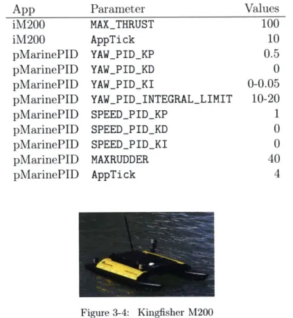
In water experiments were performed to evaluate the viability of this sort of black box model. This work was tested at the Battelle Autonomy Lab at the MIT Sailing Pavilion. While some early work was performed on Kingfisher M100's, the major-ity of the field testing was performed on Kingfisher M200's. The M200 is a small autonomous catamaran (see Figure 3-4). Propulsion is provided by two waterjets. Steering is controlled using differential drive. The frontseat contains interface layers to the thrusters and navigation equipment. Although the front seat can accept indi-vidual thruster commands from the backseat, it lacks heading and speed controllers. These functions are instead performed by pMarinePID, a MOOS application imple-menting a basic PID controller for heading and speed. Key configuration parameters
affecting vehicle maneuvering characteristics are listed in Table 3.1.
Table 3.1: Key M200 configuration parameters affecting maneuverability. In tests for this work, the following parameters were used unless otherwise specified.
App Parameter Values
iM200 MAXTHRUST 100 iM200 AppTick 10 pMarinePID YAWPIDKP 0.5 pMarinePID YAWPIDKD 0 pMarinePID YAW_PID_KI 0-0.05 pMarinePID YAWPIDINTEGRALLIMIT 10-20 pMarinePID SPEED_PID_KP 1 pMarinePID SPEEDPIDKD 0 pMarinePID SPEEDPIDKI 0 pMarinePID MAXRUDDER 40 pMarinePID AppTick 4 Figure 3-4: Kingfisher M200
box yaw model like that described in 3.5. Two sets of input data were used. The first, shown in Figure 3-5, consisted of several discrete turns. The second, shown in Figure 3-6, was a persistent excitement of the vehicle's heading. In both data sets, the desired vehicle speed was constant at 1.5 m/s.
No filtering was performed on the data. For the discrete turns in particular, non-trivial low frequency noise is apparent in the heading data. This is attributed to environmental effects. Filtering the input used for parameter identification might improve the performance of the model; this was not investigated.
The asynchronous nature of MOOS publications (see Chapter 4) means that data logged from a vehicle must be resampled to be suitable for use in linear least squares identification of the model coefficients. The minimum relevant application frequency was 4 Hz (pMarinePID). Other relevant applications, such as iM200 (providing the navigation data) and pHelmIvP (publishing desired heading) were operated at 10 Hz. To remain within the limits of the actual publications, data was resampled to 4 Hz. To resample, each relevant variable was linearly interpolated between logged values to obtain a value for each synchronous time step.
Ten seconds of history was used, corresponding to 40 samples in E and
4.
Further discussion of model form is given in Section 3.4.3.Trajectories simulated by modeling heading changes (as described in Section 3.4.1) are given in Figures 3-7 and 3-8. Both predictions are calculated from the point where the desired heading has changed but the control system has not yet responded (i.e. the first sample where DESIREDHEADING changes). In both cases the model is stable and eventually converges to the new desired heading. While it under predicts the heading change at each time step, resulting in a wider turn than actually observed, the predicted response is generally similar to the actual trajectory.
The speed at the beginning of the turn was assumed to be constant and was used to propagate the predicted position. If a suitable speed model were also developed and identified, a more accurate prediction could be developed. Both models were also tested using the actual speeds from the resampled logs instead of an assumed constant speed. While this provided minor improvement, the M200 speeds in this data were
360 300 4) cc C) (~v~ 240 K - 180- 120- 60-0 1 1 1 1 1 0 50 100 150 200 250 300
Time (s)
Observed heading Modeled heading Desired Heading
Figure 3-5: Using M200 In-Water Data to Identify Model Parameters: Input data for the black box system identification process. Here discrete turns are used, like those used to record AVK trajectories
relatively constant during the turns and the trajectories using actual speed data were not significantly different than those shown here using a constant speed assumption. For other cases where speed changes significantly during a turn, an accurate speed model would prove essential in developing accurate predictions.
While the model was able to predict some of the turns in its input data with some accuracy, it still needs refinement to adequately predict turns over the full range of heading changes. A comparison of results from this black box model and the AVK measured trajectory is given in Section 5.2.
3.4.3
Model Improvements
The black box approach described meets the goal of providing a predictive tool for cases where models of the vehicle's dynamics or low level control cannot easily be obtained. However, further work is necessary to evaluate whether a different
mod-240r 0 180 r 120
cc
60-I.. 0 5 10 15 20 25 30 35 40 45 50Time (s)
Observed heading Modeled heading Desired Heading
Figure 3-6: Using M200 In-Water Data to Identify Model Parameters: Input data for the black box system identification process. In this case, vehicle heading was persistently excited by intentionally varying DESIREDHEADING to prevent the vehicle from steadying on course.
eling approach could more accurately predict trajectories. In particular, techniques other that least squares should be explored for identifying the values of the model parameters. A least squares fit minimizes the prediction error for heading at the next
time increment. The actual desire, however, is to minimize error in the predicted tra-jectory. Parameter estimation techniques that allow an arbitrary cost function would
allow the entire trajectory to be considered in the estimation process.
One parameter which could be systematically varied in a more robust identification process is the number of time steps included in the model. The best choice for this parameter should also be informed by the ultimate usage of the model. Predicting the latter part of a large turn trajectory may require 10-15 seconds of history in the model. On the other hand, this may have undesirable effects on predicting the beginning of a turn if the prior 15 seconds have significant changes. An example of the effect of model history is given in Figure 3-9. A related analysis is to determine how
E-135
4)
0" -136-cc 5-137--138- Observed Trajectory 0 Modeled Trajectory -139-42 44 46 48 50 52 54 56x coordinate (m)
Figure 3-7: Poor input data produces poor estimates: Trajectory predictions using black box model. Model coefficients were identified from the discrete turn data set shown in Figure 3-5. The initial speed is assumed to be constant throughout the turn. In this case, the model has too much delay and predicts too little heading change at each time step. The result is a trajectory prediction with a much larger advance and transfer than the actual vehicle trajectory.
much of the trajectory must be accurately simulated to achieve the desired guidance results. It may be the case that modeling only the first (say) half of the turn achieves the necessary guidance algorithm performance. The results of this analysis could be included in the cost function for an alternative parameter estimation technique, giving higher weight, for example, to accurately predicting the beginning of the trajectory. Similarly, smaller turns (up to about 90 degrees) are more relevant to effective obstacle avoidance and could be given higher weight.
It would also be beneficial to study the model's sensitivity to the size of the time step. The time step used in the input data is implicit in the coefficients identified for a model like Equation 3.5. Utilizing a different time step requires changing the model structure and repeating the identification process.
3.5
Summary
This chapter has presented two potential approaches to allow a payload autonomous guidance system to estimate the kinematics of a turn. A simple black box model for
USV yaw dynamics was developed and tested on an M200 USV. The AVK approach
for directly measuring turn kinematics serves as the basis for the data collection procedure outlined in the next chapter.
18 --18 - Observed Trajectory -18.5 - Modeled Trajectory _ 19 - -19.5- -20-" -20.5 -00
o
-21/ 0 -21.5--22 -22.5 -23 I 28 29 30 31 32 33 34 35 36x coordinate (m)
Figure 3-8: Persistent excitation improves predictive capability: Trajectory prediction using black box model. Model coefficients were identified from the persistently excited data set shown in Figure 3-6. The initial speed is assumed to be constant throughout the turn. Compared to Figure
3-7, the prediction has much better agreement with the observed trajectory, but has a lesser the
same problem under-predicting heading change, resulting in a modest over-estimate of advance.
1.15- 1.10-I 1.05-U 1.00-0.95 -0 .) 0.90- 0.85- 0.80-.0 2 4 6 8 10 12
History in Model (sec)
Figure 3-9: Evaluation of model time scale in prediction accuracy: The accuracy of the trajectory prediction generated by the model depends directly on the amount of history included. The actual (blue) turn shown in Figure 3-8 was predicted by models with varying amounts of history. The mean squared error between each point on the predicted trajectory and the observed trajectory is shown for each prediction. It should be noted that the minimum MSE is for only one turn and does not necessarily imply an optimum choice across all heading changes.
Chapter 4
MOOS Applications and Behaviors
Data collection for the AVK approach described in Chapter 3 has been implemented in MOOS-IvP here. A brief general description of MOOS-IvP is given. More detail is available in [5].
4.1
MOOS-IvP
The Mission Oriented Operating Suite (MOOS) serves as middleware, allowing vari-ous applications to communicate with each other. For a typical autonomvari-ous vehicle mission, applications for communication, sensing, data logging, and guidance would communicate and share data through the MOOS database (MOOSDB). In a payload autonomy architecture, an interface application to communicate with the front seat computer would also be present.
MOOS applications share data through a publish and subscribe architecture. A
typical exchange of data relevant to this work is as follows: GPS data is processed in the front seat navigation system and shared to a MOOS interface application such as iM200. This application does any additional required processing such as conversion to local grid coordinates and posts a message such as NAVX = 10.5 to the MOOSDB.
An application interested in navigation data subscribes to the variable NAVX and receives a message from the MOOSDB containing the value of the variable as well as useful metadata such as the publishing application and time of publication. Some
discussion of the impacts of this data exchange architecture is given in Section 5.1. For autonomous vehicles, one of the most important functions for MOOS applica-tions is vehicle guidance. In MOOS-IvP, this role is fulfilled by pHelmIvP ("the helm"), a behavior-based architecture where action selection among competing behaviors is achieved with multi-objective optimization using interval programming
[6].
The helm makes guidance decisions by solving an optimization problem framed by one or more behaviors. Typical behaviors include waypoint following, (static) obstacle avoidance, and contact avoidance. Each behavior generates an objective function, assigning a utility value to each possible combination of speed and heading. (Although simple behaviors might only produce an objective function for one of these variables).Of note for this work, the helm is configured with a specific discretization of the
decision making domain. A typical configuration would be discretizing the heading domain to 1' and the speed domain to 0.1 m/s. Recalling Section 3.3.2, this illustrates the need for methods such as interpolation to reduce the number of discrete heading change and initial speed combinations that are empirically tested to populate the table.
4.2
TurnSequence Class
The TurnSequence C++ class is the fundamental data structure used in this work. It contains the meta-information needed to identify a turn, namely the turn speed and heading change. The turn trajectory is recorded using a list of X/Y coordinates.
A TurnSequence has two fundamental purposes. First is to serve as a record
of a turn performed in order to ascertain vehicle kinematics. The TurnSequence is passed to functions to fit a polynomial to the data (Section 3.3.2). In order to provide consistent input to the curve fitting functions, the standard orientation described in Section 3.2 has been applied to TurnSequence's: the turn starts at the origin with an initial heading of North and the turn is made to the right. The turn records obtained during a data collection mission will be initiated at arbitrary X/Y coordinates and could be either left or right hand turns. The class includes functions to rotate,
translate, and reflect an arbitrary turn to match the orientation convention.
When rotating the TurnSequence to be North facing, the turn is rotated based on the instantaneous heading at the start of the turn. If the vehicle is steady on the initial heading, the normalized turn trajectory will initially be perfectly vertical (due North), whereas if the vehicle had an initial yaw rate, the trajectory will diverge.
The TurnSequence class is also used to express the piecewise linear approximation of the polynomial fit to the source data (discussed in Section 3.3.2). The meta-data is the same as the original turn record, but the list of points is simplified. This type of TurnSequence is generated either by processing raw data or using the interpolation process described in Section 3.3.2. To evaluate vehicle trajectories with respect to obstacles, the rotation, translation, and reflection functions are used to match the TurnSequence to the vehicle's pose.
4.3
pDynamicsMonitor
pDynamicsMonitor is a MOOS App designed to coordinate the data collection mission run to collect AVK trajectories. It interacts with the ConditionSet, ConstantHeading, and ConstantSpeed behaviors. These behaviors are described in Section 4.4 and the overall coordination in the mission is described in Section 4.5. pDynamicsMonitor is configured with a range of heading changes and speeds directs each combination to be conducted. As turn data is collected, the resulting TurnSequence is logged for post processing.
4.4
Behaviors
MOOS-IvP utilizes a behavior based architecture. This allows each goal (such as waypoint following or collision avoidance) to be expressed individually. While this architecture generally performs multi-objective optimization from multiple competing behaviors, the data collection process was utilized several discrete helm modes, with no competing behaviors active simultaneously. This arose from the need to measure
the response of the vehicle (controller and physical) with precisely known input from the backseat. Several existing behaviors were either utilized or modified, and two new behaviors were written.
4.4.1
ConditionSet
Section 6.2 discusses the importance of defining a specific vehicle state associated with the start of a particular turn. The ConditionSet behavior exists to establish the required state. For the simplest case, this means establishing a desired speed and a steady course. Steady course is determined by calculating yaw rate from NAVHEADING postings.
tk - tk_1
Differentiating discrete heading readings to determine yaw rate was found to gen-erate a highly noisy yaw rate, even in simulation. To smooth the data, a moving average was used to reduce the effect of noisy heading data.
1n-1
/avg = - En-k (4.2)
k=O
Where n is the window size of the filter. It was found that with navigation data published both at 4 Hz (in simulation) or 10 Hz (on the m200), a window size n = 5 gave good results.
ConditionSet is configured with a desired speed and acceptable speed tolerance and a maximum yaw rate. On becoming active, ConditionSet notes the current course. Until the configuration thresholds are achieved, ConditionSet generates an objective function to maintain course and achieve the desired speed.
4.4.2
Operating Region and Container
The OpRegion behavior is distributed with MOOS-IvP. It is configured with a polygon that the vehicle is to remain within. If the vehicle exits the polygon, it is shut down.