Measuring corrosion levels of ductile iron pipes using scanned images

(1)

Publisher’s version / Version de l'éditeur:

Vous avez des questions? Nous pouvons vous aider. Pour communiquer directement avec un auteur, consultez la première page de la revue dans laquelle son article a été publié afin de trouver ses coordonnées. Si vous n’arrivez pas à les repérer, communiquez avec nous à PublicationsArchive-ArchivesPublications@nrc-cnrc.gc.ca.

Questions? Contact the NRC Publications Archive team at

PublicationsArchive-ArchivesPublications@nrc-cnrc.gc.ca. If you wish to email the authors directly, please see the first page of the publication for their contact information.

https://publications-cnrc.canada.ca/fra/droits

L’accès à ce site Web et l’utilisation de son contenu sont assujettis aux conditions présentées dans le site LISEZ CES CONDITIONS ATTENTIVEMENT AVANT D’UTILISER CE SITE WEB.

Research Report (National Research Council of Canada. Institute for Research in Construction), 2008-11-01

READ THESE TERMS AND CONDITIONS CAREFULLY BEFORE USING THIS WEBSITE.

https://nrc-publications.canada.ca/eng/copyright

NRC Publications Archive Record / Notice des Archives des publications du CNRC :

https://nrc-publications.canada.ca/eng/view/object/?id=842b0ab8-bbbb-473c-9890-5a64bfd1045a https://publications-cnrc.canada.ca/fra/voir/objet/?id=842b0ab8-bbbb-473c-9890-5a64bfd1045a

NRC Publications Archive

Archives des publications du CNRC

For the publisher’s version, please access the DOI link below./ Pour consulter la version de l’éditeur, utilisez le lien DOI ci-dessous.

https://doi.org/10.4224/20374408

Access and use of this website and the material on it are subject to the Terms and Conditions set forth at

Measuring corrosion levels of ductile iron pipes using scanned images

(2)

http://irc.nrc-cnrc.gc.ca

M e a suring c orrosion leve ls of

duc t ile iron pipe s using

sc a nne d im a ge s

R R - 2 6 8

M a k , H . ; W o n g , B . ; K r u i t h o f , S . ; K r y s , D . ; L i u , Z .

N o v e m b e r 2 0 0 8

(3)

Executive Summary

This report documents the findings and the results of an engineering exercise to develop a process to measure the corrosion depth of buried samples from their scanned images before and after burial. The recommended method consists of 5 steps which combine the power of a Konica Minolta scanner, PolyWorks and software developed in Matlab. PolyWorks is mainly used as a human interface for manipulating and aligning point cloud data sets. The use of PolyWorks reduces software development to a minimum. Software developed in Matlab is mainly for image transformation and corrosion depth/volume calculation.

Since the corrosion measurements are planned to span from 5 to 20 years, the proposed process is developed with long term viability in mind. Both the Minolta scanner and PolyWorks can be replaced with other systems providing similar functionalities. The interface files are ASCII based which is universally acceptable. All theories, algorithms and engineering principals involved are documented in sufficient details in the Appendix sections so that the software code can be re-implemented in any form possible if Matlab becomes obsolete.

The practicality of this process has been verified using three simulated laser-scanned images each of two samples at corrosion depths of 0.08 mm, 4 mm and 4 mm with +/-5% noise added. In this way, the recommended method and software developed in Matlab is also verified.

The calculation of the corrosion volume is one of the goals of this exercise. It is found that the corrosion volume derived from a single image scanning method is not a comparable quantity between any two corrosion measurements. This is because the scanning angle is uncontrollable when samples are scanned years apart. This varies the visibility of the boundaries of the sunken corrosion surface at each scan. Instead, it is proposed to use the mean corrosion depth, defined as the total corrosion volume per unit corrosion area, for this purpose. Multiple scanning of the sample will correct this problem, but it will involve more complicated image stitching operations in PolyWorks. This is left as a future improvement of the current method.

Logically, the accuracy of this method depends heavily on the surface treatment of the corroded surface. Surface dirt and loose particles have to be removed in a way that does not damage the actual underlying metal surface. Surface rusts that cannot be removed will introduce errors to this method.

In conclusion, the recommended method has measured the simulated corrosion depths with accuracies over 95%. It is an acceptable process.

(4)

1 Background

1.1 The Project

The Buried Utilities Group, Urban Infrastructure Program, is conducting a project to assess the degree of corrosion of buried ductile iron pipes. The project uses several sensors, CORROSOMETER® Corrosion Probes, which are designed to estimate the corrosion level of a ductile iron pipe. The sensors contain a sample of ductile iron, which is exposed to the same elements as the target ductile iron pipe. The corrosion on this exposed area will reflect the degree of corrosion on the buried pipes. These sensors are designed to be read by a corrosometer, CORROSOMETER® Portable Instrument, which measures electrical resistance across the exposed ductile iron sample. As the sample corrodes there is less material so the resistance of the sample increases. The problem is that there seems to be little experimental data showing the effectiveness and

characteristics of these specific sensors. So a series of tests have been set up to evaluate the characteristics of the sensors.

Initial tests include leaving these sensors in controlled environments beside ductile iron pipes. The problem with this is that the samples will take 5 to 20 years to corrode. So another set of tests has been developed that will use electrolysis to increase the corrosion rate of the samples. This will allow the samples to corrode in months rather than years. To confirm that the electrolysis is a controlled environment and the results can be reproduced, a set of our own samples was manufactured that can be used to test the environment. These samples are just sections of ductile iron pipe that have an exposed surface that is the same surface area as the corrosion sensors. Once the results show that the electrolysis can be performed as to yield the same results each time, then the

experiment will be used on the actual corrosion sensors.

In order to evaluate the amount of corrosion, a set of different test methods are needed. For the electrolysis test, three different techniques are used to gather data on the amount of metal loss. The first method is to compare the weight of the sample before and after the experiment. The difference in weight will reflect the total metal loss. The second technique will be to measure the number of electrons that were removed from the sample using electrolysis and then calculate that total weight loss. The problem with these techniques is that they will tell us how much metal loss there was, but there is no

information to say where it was lost. This third technique is to use laser-scanned images to measure the corrosion rate. Dennis Krys has also developed a basic program in Matlab to measure the corrosion depth of any two laser-scanned images. This technique will

(7)

exposed surface of a sample. The corrosion depth across the complete area of the exposed surface, the distribution and the total corrosion volume must be calculated. CCCT has been provided with two samples (Sample A & Sample B as shown in Appendix C.1) to perform the study.

Based on this approach, CCCT has:

• Recommended a way to improve the accuracy of image alignment of the scanned images by incorporating abrupt changes to the otherwise gentle geometric shape of the samples. This is achieved by using a few pieces of Lego blocks to be installed in the surrounding area of the exposed surface (See Appendix C.1). • Performed the scanning of the samples using the Konica Minolta 3D Digitizer

VIVID 910.

• Developed a method to combine the image alignment capability of PolyWorks and image processing power in Matlab to derive the delta of any two scanned images.

• Verified the method by using three simulated corrosion scanned images of each sample with corrosion depths of 0.08 mm, 4 mm and 4 mm with noise.

The goal of this document is to record the methods, the results and the engineering

principles / theories involved. As the methodology proposed in this project has a potential time span greater than 10 years, it is necessary to document all relevant information in very simple terms so that they can be referred to in future. The image files, due to their size, are not included in this document. They, together with the Matlab code, are stored electronically in the shared drives at the NRC London site. The files are backed-up periodically; their archives are kept for a long time and are available on request.

1.3 The Technology & Challenges

The challenge of this project is to find the offset distances (profile) of the corroded surface from its original exposed position. However, one cannot find this distance by simply subtracting the points in the scanned images of the corroded object and the original object, because each image sits in its own 3D space. The origin, the viewing angle (scan angle) and coverage area of any two scanned images may be different because of the individual setup.

The general procedure to calculate the offset distance(s) of two scanned images is as follows:

1. Align the two geometric shapes represented by their point cloud data sets by fitting local surfaces to them.

2. Lay a common grid to the corresponding surfaces and find out all the grid points on these surfaces.

3. Calculate the z-distance between corresponding grid points of the two sets of surfaces.

4. Analyze the distribution of the offset distances of the exposed area before and after corrosion which will reflect the nature of the corrosion.

(8)

The alignment (or some times called registration) of two cloud point data sets in Step 1 is still a hot research topic. Typically, the process is divided into two stages:

1. Crude pre-alignment: The intention of this operation is to roughly put the two images in the same orientation by translation and rotation. Many researchers are still working on this area to provide an automatic way to pre-align two point cloud data sets. Commercial tools, e.g. PolyWorks, usually use a semi-manual method, which require the operator to pick a set of identical points (landmarks) from the two images and then the software will perform the rough alignment1.

2. Fine alignment: The goal of this operation is to move the two point clouds relative to each other so that the sum of the square distances between the two images is minimum (least square method). The golden standard process used in the field is the Iterative Closest Point (ICP) algorithm which is also implemented in

PolyWorks.

Since the ICP will attempt to average the distance of the two images, the corroded surface will introduce errors in the fine alignment stage. Hence, the corroded surface has to be excluded in the image alignment step. Once the alignment is achieved, one needs to find out the transformation matrix that the alignment algorithm has used and re-apply it to the points of the corroded area.

The scanning operation of the original surfaces of the samples is very important in this method, because it produces the images to which all subsequent images of corroded samples have to be compared. As the method to calculate the corrosion depth developed by Dennis is based on the delta of the z-values of the grid points, the scanning has to be performed as close to the surface normal of the samples as possible. Since it is very difficult to be exact, the orientation of the scanned images needs to be determined and rotated accordingly, using image processing techniques so that their surface normals align with the z-axis before the corrosion depth can be calculated.

One intention of this project is to calculate the corrosion volume of the sample after a period of burial. To do this, one has to find the actual boundary of the corroded surface and the corrosion depth at each point. Unfortunately this may not be possible, especially for sunken surfaces, because the scanning angle is not controllable in our case. Some part of the actual boundary of the corroded surface may not be visible in the scan.

To overcome this challenge, it is proposed to use the mean corrosion depth of the

corroded surface instead. The mean corrosion depth is the total corrosion volume per unit corrosion area. In this way, it is independent of the corroded surface boundary. To

(9)

Appendix A.3 and Appendix A.4. The algorithm to determine the boundary of the exposed area used in mean corrosion depth calculation is documented in Appendix A.5 and the corrosion volume calculation in Appendix A.2.

(10)

2 The Proposed Process

Figure 1 and Figure 2 show the complete operation flow of this process. For the sample before corrosion (refer to Figure 1):

1) Scan the original sample using the Konica Minolta 3D Digitizer VIVID 910. The scanning should be done at the minimum distance (or maximum resolution) of the scanner. The Digitizer’s line of sight (z-axis) should be aligned closely with the sample surface normal. This generates the image file IMO.

2) Load the image IMO into PolyWorks:

a. Cut off the points in the exposed area of the sample and save it as image file IMO_hole.

b. Cut off all the points of the IMO image leaving only the exposed area and save it as image file IMO_exposed.

Image scan

IMO

Original Sample

Cut out exposed area

IMO_hole Color code: • PolyWorks operation • Matlab operation • File_name

STEP 1

STEP 2

IMO_exposed

(11)

of the scanner. The Digitizer’s line of sight (z-axis) should be aligned closely with the sample surface normal. This generates the image file IME.

2) Load the image IME into PolyWorks, cut off the points in the exposed area of the sample and save it as image file IME_hole.

3) Load both IMO_hole2 and IME_hole into PolyWorks and use the point cloud alignment tool to align IME_hole to IMO_hole. Save the aligned IME_hole to file IME_hole_aligned.

4) Use Matlab to calculate the corrosion depth

a. Edit the front part of main6 in Matlab to provide

i. the input file directory and file names for IMO_exposed, IME_hole, IME_hole_aligned and IME, and

ii. the output file directory and file name for IME_aligned, IMO_exposed_rotated1 and IME_exposed_rotated. b. Run main6 in Matlab

c. Log down the analysis results displayed on the screen and the figure displaying the results of corrosion depth histogram and distribution. 5) Use PolyWorks to display the delta of IMO and IME_aligned and to inspect

IMO_exposed_rotated1 and IME_exposed_rotated to check if the area used for corrosion calculation is properly set.

2

(12)

Corroded Sample

Image scan

IME

Cut out exposed area

IME_hole

IME_hole_aligned

And apply to IME, Extract the boundary of IMO_exposed to extract IME_exposed to calculate the corrosion distance & Derive Xform matrix from IME_hole to IME_hole_aligned volume. IME_aligned

STEP 1

STEP 2

STEP 3

STEP 4

STEP 5

IMO_exposed_rotated1 IME_exposed_rotated

Align with IMO_hole

Display corrosion distance distribution

Color code:

(13)

3 Test Results

In order to test the process and all software tools developed, three simulated corrosion scanned images are created mathematically3 to simulate the corrosion depths of 0.08 mm, 4 mm and 4 mm with 5% noise added respectively to the exposed area of Sample A and Sample B. This section documents the test results of the process using these simulation files.

3.1 Sample A

The data measured from Sample A:

• The surface normal of the exposed surface is found to be at 2.43o

to the z-axis. After re-orientation, the angle becomes 0.002o.

• The vertices of the inner cropping polygon used in all corrosion calculations for Sample A are 3.7963, 29.7675), (43.2575, 26.9300), (42.2943, 17.9787) and (-3.8680, 19.3511).

3.1.1 0.08 mm Simulated Corrosion Depth

The screen captures of the results for processing the 0.08 mm simulated scanned image are included in Appendix C.3 section C.3.1.

Here are the results obtained from the process:

• The min, median, max, and std of the corrosion depth are -0.014 mm, 0.083 mm, 0.163 mm and 0.088, respectively.

• The total corrosion volume measured within the cropping polygon is 37.06 mm3

. • The total corrosion area within the cropping polygon is 449.27 mm2

. • The mean corrosion depth = 0.082 mm.

• Method accuracy = 1 0.082 0.08 100% 97.5% 0.08 − ⎛ ₋ ⎞_× ₌ ⎜ ⎟ ⎝ ⎠

3.1.2 4 mm Simulated Corrosion Depth

The screen captures of the results for processing the 4 mm simulated scanned image are included in Appendix C.3 section C.3.1.

• The min, median, max, and std of the corrosion depth are 3.799 mm, 4.032 mm, 4.269 mm and 0.052, respectively.

• The total corrosion volume measured within the cropping polygon is 1811.92 mm3.

• The total corrosion area within the cropping polygon is 449.31 mm2

3

The scanned image of Sample A is taken and all the points in the exposed area are isolated using PolyWorks. Matlab is used to (1) find the angle of the surface normal to the z-axis, (2) rotate the exposed area accordingly, (3) add 0.08 mm, 4 mm and 4 mm + 5% random noise, respectively to the z values of these points and then (4) rotate the exposed area back to generate the simulation scan files.

(14)

• Method accuracy = 99.25%

3.1.3 4 mm Simulated Corrosion Depth with +/- 5% Noise

3.2 Sample B

The data measured from Sample B:

• The surface normal of the exposed surface is found to be at 6.64o

to the z-axis. After re-orientation, the angle becomes 0.004o.

• The vertices of the cropping inner polygon used in all corrosion calculations for Sample B are 14.2617, 80.5095), (35.0287, 78.0985), (35.3734, 68.0502) and (-14.3429, 70.2161).

3.2.1 0.08 mm Simulated Corrosion Depth

The screen captures of the results for processing the 0.08 mm simulated scanned image are included in Appendix C.3 section C.3.2.

• The min, median, max, and std of the corrosion depth are -0.219 mm, 0.083 mm, 0.690 mm and 0.032, respectively.

• The total corrosion volume measured within the cropping polygon is 41.83 mm3

. • The total corrosion area within the cropping polygon is 500.34 mm2

• Method accuracy = 95%

(15)

3.2.3 4 mm Simulated Corrosion Depth with +/- 5% Noise

(16)

4 Discussion

From the test results, it is found that:

1. The accuracy of this method depends heavily on the surface treatment of the buried sample prior to the measurement. One has to remove all dirt and loose particles (e.g. rust) from the metal surface without damaging the integrity of the underlying metal surface. When metal rusts, it expands in volume. The rust on the corroded surface will introduce errors in the mean corrosion depth calculated. 2. The corrosion volume derived from a single image scanning is not a comparable

quantity between any two corrosion measurements. Instead the mean corrosion depth is a better means for this purpose. This is because the scanning angle of a corroded sample, performed in subsequent scans years apart, is not controllable. The resulting point cloud image of the corrosion area will differ between scans, especially for sunken surfaces, where there may be areas that are visible in one scan and not in another. Even if one applies image processing techniques to align the corroded surface with the original one and crop both with the same outline, the resulting corroded surface may still differ between scans. Since the corrosion volumes are calculated based on these corrosion areas, the corrosion volume thus calculated cannot compare one from the other. The mean corrosion depth,

however, being the ratio of the corrosion volume per unit corrosion area, is independent of the corrosion area from one scan to another. It is a better measure to compare degree of corrosion with. A multiple scan approach may solve this problem. It is left as a future development of this method.

3. The test results have shown that this method can measure the simulated corrosion depth, even with noise introduced, above 95% accuracy. Better results are

obtained for Sample A (97%, 99% and 99%) than Sample B (95%, 100% and 98%).

4. The histogram of each corrosion simulation test should theoretically consist of one value only, except the ones with normally distributed random noise added. The deviation from the theoretical value is due to several factors: the non-planar nature of the exposed surface, the closeness of the edges of the selected exposed area to the protected area and the way the corrosion depth is calculated, using the Matlab method.

a. The non-planar nature of the exposed surface, especially Sample B, prevents a perfect alignment of the surface normal to the z-axis in every part of the surface. In creating the simulation files, the simulated corrosion depth is added to the z-values of all the points in the aligned exposed area of the original scanned image. However, due to the local surface normal variations, the result is not a straight offset movement of the exposed

(17)

amount of corrosion depths from 2.0 to 3.5 mm as seen in the histogram of Sample B with 4.00 mm corrosion depth +/- 5% noise added (Appendix 0). The diagrams on the right show the

different views of the cropped exposed surface area in this case. The points concerned are enclosed in the blue polygon. However, they do not affect the accuracy of the corrosion depth measurement. This problem can be corrected by selecting a smaller exposed a to show this is a possible outcome. c. The interp

rea for Sample B. However, this is not done olation of the scan points into the common grid points using local cubic surfaces introduces variances into the intended result. The median values and the tight σ values of the corrosion depth in the 0.08 and 4 mm test cases have shown that the method works relatively well. The Matlab code for analyzing the corrosion depth results are written to handle 5.

to cise, normally distributed random noises have been

introduced,

ility of this process, though it cannot be validated, has wer

at

t method provides only limited data on corrosion features, e.g. pits. It

or corrosion depth variations. The histogram, statistical data and 2D distribution display of the measured corrosion depth, should reveal valuable information as the nature of the corrosion.

6. During the engineering exer

introduced to the corroded surface of the simulated scanned images. Unfortunately, it occurs that if too high a noise level (e.g. +/- 25%) is

PolyWorks will not be able to create an underlying surface to these scan points, hence the method developed will not work. Hence this exercise restricts itself to +/-5% as a maximum.

7. The long term applicab

reasonable assurances. In years to come, the scanner can be replaced with a ne one as long as it can output the point cloud image in text file format. PolyWorks can be replaced by any packages having the same functionality to manipulate point cloud data. The Matlab code may not run because of a new language form or platform changes. However the theories and algorithms involved will remain the same. One can easily recode the program to suit the new language format required.

8. The curren

provides the minimum, maximum and distribution of the corrosion depth. One can recognize the pits on the surface using the corrosion depth distribution diagram. In future, it may be feasible to extract more information about pits other corrosion features such as the location, size and depth.

(18)

5 Future Improvements

The investigation is by no means complete given the time constraint. There are possible future improvements of the current proposal.

The proposed method is based on a single scanned image of the samples. Unfortunately, the visibility of the boundaries of a sunken surface is not consistent for scans to be performed years apart. This is because the scanning angle is not controllable. At a different angle, the bottom edges of the sunken surface may not be visible from the scanner. To overcome this problem, a multiple scan operation can be used. Each sample will be scanned multiple times at different angles to ensure the entire sunken surface including the transition slops, is covered. PolyWorks can be used to stitch all these point cloud images together to create one single scanned image. This will replace the IMO and IME files in Step 1 of the process. In Step 4, the current Matlab software uses a smaller (10% reduction) inner polygon to calculate the corrosion volume. With the multiple scans approach, the Matlab software should be modified to use an enlarged outer and inner polygon for the corrosion volume calculation. The enlarged polygons are to ensure that the transition slops and bottom corrosion surface are fully covered for corrosion volume calculation. A possible enlargement factor can be α =1.3 and α =1.1 for the outer polygon and inner polygon respectively. The rest of the process will remain the same. The current method avoids the determination of the actual boundaries of the sunken surface. Instead, it requires the operator to identify them in the original sample image (Step 2). An alternate approach will be to use image processing capabilities in Matlab to detect the actual irregular boundaries of the exposed surface and the transition slops. This approach will require multiple scanning of the exposed surface.

The current method uses PolyWorks to align the before and after corrosion images with the exposed area removed (IMO_hole and IME_hole). This is required because

PolyWorks does not allow users to specify areas to ignore during the alignment process. One can find a different software tool to provide this capability or it can be implemented in Matlab. In this case, the entire process can be greatly simplified. The operator will just scan the sample and run the Matlab program to get the results.

The current method provides only limited data on corrosion features, e.g. pits. It provides the minimum, maximum and distribution of the corrosion depth. One can recognize the pits on the surface using the corrosion depth distribution diagram. In future, it may be feasible to extract more information about pits or other corrosion features such as the location, size and depth.

(19)

6 Conclusion

In this engineering exercise, a usable process has been developed to measure the

corrosion levels of buried samples. This method is based on existing equipment at hand. combines the powers of our Konica Minolta scanner, PolyWorks and Matlab. The It

proposed process has long term sustainability since the engineering theory is well documented. It can be easily modernized into a newer form making use of newer equipment and software tools at the time. Comparing corrosion volumes for each corrosion measurement is still a challenge yet to be resolved. However, the method developed has achieved accuracy over 95% in measuring the mean corrosion depth of the sample.

(20)

(21)

A.1 Image delta of two point cloud data sets

.1.1 The Concept

he key engineering problem of this evaluation is how to calculate the offset of the orroded surface scanned image from the original surface scanned image of the same uried sample. As the corrosion may take considerable time (e.g. 5 years) to occur, the

o image scans have to be performed independently, some years apart. This makes it possible to scan the samples in an identical setup. The scanned images will have ifferent scan origins, 3D spaces and total number of scan points. The scan lines and oints of one image will not align with the other. So the first step is to align the 3D space f the two scanned objects. Even though the two 3D spaces become the same, the scan nes and scan points are not aligned. Hence, the delta of the two scanned images cannot e calculated by finding the difference of the z values. The two surfaces have to be fitted etween the points and the corresponding positions have to be found to calculate the

age delta.

he method4 developed in this exercise is ased on how 3D surfaces are represented in

atlab. A 2D regular grid is created in the sho

co

space on an X-Z plane. The grey and brown dots represent the point cloud data of the original surface and the corroded surface respectively. The grey and brown curves represent the local fitted curves (cross section of fitted surfaces) to the two point cloud data sets. The red triangles represent

the interpolated points (z values) of the fitted curves at the x grid positions. The blue lines are the corrosion depth (image delta) that will be calculated.

The XY gridding of the point cloud is effectively a sub-sampling of the point cloud data. It reduces the computational points from 96K to a manageable size which is controllable by the resolution of the grid. The z-value delta is a simple matrix operation between the grid points. One important note is that the two scan point clouds may cover different areas because the two images are scanned with different scanning angles. So some grid points of one image may not have corresponding points in the other on which to find the delta. This is especially true around the perimeters of the two point cloud data. This has to be taken care of in the image delta calculation.

A T c b tw im d p o li b b im T

Figure 2: Image delta

z

x b

M

XY plane of the two point cloud sets as wn in Figure 2. Figure 2 illustrates the ncept on a 2D cross section of the 3D

4

(22)

A.1.2 The Implementation

Matlab provides a good number of existing functions to support the grid generation and interpolation of the point cloud data into a grid. The interpolating function allows users

rface es) the n urface gradient at it ch:

the entire region (area enclosed in dotted lines uced area in contour with the external to select some simple surfaces to fit the local region of points. In the code, a cubic su is used for this purpose.

The common grid for the two point cloud data sets is created with a size based on the minimum and maximum x and y values of the combined two data sets. The grid (z valu values of each point cloud sets are represented in an m-by-n matrix, corresponding to x-y positions of the grid. Since the grid space is larger than or equal to the point cloud space, the z values of the uncovered area in the matrix are filled with NaN (not a number, a special value in Matlab). The corrosion depth is found by subtracting the two matrices. The resulting m-by-n matrix of the image delta is not totally numerical. It contains a large number of NaNs, especially around the edges. In the calculation of the corrosion volume, these values have to be skipped.

It is found that the surface fitting function i Matlab, griddata, may generate

abnormalities at the region around the edge of the interpolated surface. Depending on the local s the edge area, the resulting surface may rise up or fall down in the edge regions introducing erroneous results in the image delta calculation. To work around this problem, is recommended to use a two steps approa 1. The image delta is calculated over

in the figure) and

2. The result is interpreted within a red

boundaries (area enclosed in solid lines in the figure).

From the experimental results, it is found that a 10% margin will be sufficient for this urpose.

(23)

A.2 Corrosion Volume and Mean Depth Calculation

A.2.1 Calculation

In the corrosion depth calculation, a regular grid (square) is needed to sample the two itted images surfaces. Th

f e corrosion depth at a grid point is calculated as the z-distance between the two surfaces at the corresponding grid sample points on the two surfaces. This creates a number of hexahedrons with square cross-sections. When the grid resolution is high, the corrosion volume can be approximated by the summing of the volumes of all these hexahedrons.

Take one of the hexahedron as example:

i

v

Δ =cross section area x average height h1

2 h h3 4 h 4 2 1 1 4 i j j v s h = Δ = ×

∑

,

where s is the side of the square cross-section Hence, the total corrosion volume,

i

V v

al area.

E ≈

∑

Δ i,

And the total corrosion area, A_E = × when s2 image delta.

The mean corrosion depth,

re n=total number of hexahedrons in the

E E E V h A = A.2.2 Implementation

Unfortunately, even though the before and after corrosion scans can be perfectly aligned m

using i age processing techniques, the two images may still have different coverage areas. This is because the two scan may be performed at slightly different scan angles and

o find the total corrosion volume and the mean corrosion depth, one has to scan every exahedron in the image delta, check for its validity (i.e. having 4 real heights) before

mming its volume and area towards the total. The mean corrosion depth thus derived is f higher accuracy than the method documented in Version 1 of this document.

the resulting images may have scan points existing in one scan and not in another. The image delta thus derived from Appendix A.1 will have invalid values (NaNs) in some

ocations. l T h su o

(24)

A.3 Fitting a plane to the image

A.3.1 The Theory

The image is a set of N points in 3D space

(

xi yi zi

)

_N. A plane in 3D space is defin

by Ax+By Cz+ + = , in general. To fit a plane through the point cloud is to find the D 0 set of coefficients

(

A B C D

)

that will provide the least error through all the N points. One should note that there is not a unique set of

ed

(

A B C D

)

for this plane. If ll 4 numbers are divided with a constant, the plane remains the same. This problem is a

ultiple variables.

Let l form

a

classical linear5 regression problem with m

: z=a0+a x1 +a y2 us rewrite the plane into a more usefu

When a point from the point cloud points is substituted into this plane: , where is the error.

e least square sense, will be when i 0 1 2 i i i i i

(

)

e = −z a +a x +a y z =a +a x +a y +e e 0 1 2 i i i i

The optimal solution of the a’s, in th

(

)

2 0 1 1 N N i i i i i E e z a a x = =

∑

=

∑

⎡_⎣ − + ⎤_⎦2 2 1 i a y = + is minimum, i.e. at 0 1 0, 0 E E a ∂ ₌ ∂ ∂ ∂a = and ₂ 0 E a ∂ ₌ ∂ Giving:

(

0 1 2

)

1 0 2 _i _i i z a a x a a = = − − − − ∂

∑

0 N i E y ∂ ₌

(

)

(

)

0 1 2 1 1 0 1 2 1 2 2 0 2 0 N i i i i i N i i i i i E x z a a x a y a E y z a a x a y a = = ∂ _{= −} _{− −} ₋ ₌ ∂ ∂ _{= −} _{− −} ₋ ₌ ∂

∑

iving: G 0 2 1 2 2 i i i i i i i i i i i i i i i N x y a z x x x y a x z y x y y a y z ⎡ ⎤⎧ ⎫ ⎧ ⎫ ⎪ ⎪ ⎪ ⎪ ⎢ ⎥ ₌ ⎨ ⎬ ⎨ ⎬ ⎢ ⎥ ⎪ ⎪ ⎪ ⎪ ⎢ _{⎥ ⎩ ⎭} ⎣ ⎦ ⎩ ⎭

∑

6 (1.1)

(25)

Let

[ ]

1 1 1 x y 1 _i _i 1 _N _n P x y x y ⎢ ⎥ ⎢⎣ M M ⎡ ⎤ ⎢ ⎥ ₁ ₁ ⎢ ⎥ = , then ⎢ ⎥ ⎢M M ⎥ 1 N ⎥⎦ 1

[ ]

1 T i N i P x x x y y y ⎡ ⎤ ⎢ ⎥ = ⎢ ⎥ ⎢ ⎥ ⎣ L L ⎦ ⎪ ⎪_{⎩ ⎭}a₂ n

{ }

01 a A a ⎧ ⎫ ⎪ ⎪ = ⎨ ⎬,

{ }

1 i z Z z ⎧ ⎫ ⎪ ⎪ ⎪ ⎪ ⎪ ⎪ = ⎨ ⎬ L L and z ⎪ ⎪ ⎪ ⎪ ⎪ ⎪ ⎩ ⎭ M

Then equation (1.1), can be rewritten in matrix form as:

[

M

] [ ]

T

{ }

[ ]

T

{ }

P P A = P Z

{ }

A Solving for : A.3.2 Calculation nction: ⎞⎟ ⎠

The plane will be

{ }

A =

(

[ ] [ ]

P P

)

(

[ ]

P

{ }

Z

)

(1.2)

1

T − T

Equation (1.2) is easily solved in Matlab by using the matrix inverse fu

{ }

A = ⎜⎛

[ ] [ ] [ ]

P ′* P ⎞ ⎛_{⎟ ⎜}\ P′*

{ }

Z

⎝ ⎠ ⎝

(26)

A.4 Rotating an image

1 Background

In this approach, the corrosion depth at each point on the exposed surface of the sample is found by subtracting the z value of the corresponding point from the original surface.

es that the image is scanned precisely in a vertical direction. This is age ligns with the z-axis.

Calculation

age, the simplest method is to fit a plane

through the image and use th e of rotation and the

is fitted

The unit normal to the plane is

A.4.

However, this assum

impractical, in general. Hence, in order for the corrosion calculation to work, the im must be rotated so that the normal of the image surface a

A.4.2 The

To find out the general orientation of the im

e plane normal to determine the angl axis of rotation required.

Supposed a plane Ax+ through the point cloud

0

By Cz+ + =D θ

image. A normal vector

N is given by the vector

{

A B C

}

T. plane

z y ˆ n r x ˆ 2 2 2 ˆ N n C N ⎪ = _{= ⎨} / A B A B C ⎧ ⎫ ⎪ ₊ ₊ ⎬ ⎪ ⎪ ⎩ ⎭ he angle of rotation

T θ is the angle made by

with the z-axis and the axis of

formed by ction obeying the right hand rule. Hence:

ˆ n rota

{

}

ˆ 1 T z= and ˆz 0 0 in a dire

tion ˆr should be normal to the plane

ˆ n

(

)

1 ˆ ˆ cos ˆ ˆ ˆ ˆ ˆ n z n z r n z θ ₌ − _• × = ×

The transformation matrix T to rotate a point x y z ⎧ ⎫ ⎪ ⎪ ⎨ ⎬ ⎪ ⎪ ⎩ ⎭ to a new position x y z ′ ⎧ ⎫ ⎪ ⎪_′ ⎨ ⎬ ⎪ ⎪_′ ⎩ ⎭ through an

angle θ with an axis of rotation ˆ

x

r

r r

⎧ ⎫ ⎪ ⎪

(27)

(

)

(

)

(

)

(

)

(

)

(

)

2

s sin 1 cos sin

1 cos sin 1 cos cos 1 cos sin

n 1 cos sin 1 cos cos

x y z x z y x z y y z x z y x z r r r r r T r r r r r r r r r r r

(

)

(

2 1 cos rx cos 1 co ry

(

1 cos

)

r rz x rysi θ θ θ θ θ θ θ θ θ θ θ θ θ θ θ θ θ − − + + − − ⎢ ⎥ − + − + 7 θ ⎤ ⎥ ⎥⎦ ⎡ − + − ⎢ = − + − ⎢ − − ⎣ Or,

( )(

ˆ 1 cos

)

( )

ˆ sin cos

T =Sym r − θ +Skew r θ+I θ where 2

( )

2 2 ˆ ˆ ˆ x x y x z T x y y y z z ym r r r r r r r r r = × _{= ⎢} _{⎥ ,} r r r r r ⎡ ⎤ ⎢ ⎥ 0 rz ry x z y z r S r r r ⎢⎣ ⎥⎦

( )

ˆ 0 0 z x y x Skew r r r r r ⎡ − ⎤ ⎢ ⎥ =_⎢ − _⎥ ⎢₋ ⎥ ⎣ ⎦

and I is the 3x3 identity matrix.

Hence for an image _i _i _i

1 1 1 n n n x y z IM x y z x y z ⎡ ⎤ ⎢ ⎥ ⎢ ⎥ ⎢ ⎥ = ⎢ ⎥ ⎢ ⎥ M M M M ⎢ ⎥, the rota ⎣ T ⎦ ted image: * R IM =IM T

This can be checked by setting the rotati to be the x-axis, i.e. r_x 1,r_y r_z 0

7

Reference: Josef Hosckek and Dieter Lasser, “Fundamentals of Computer Aided Geometric Design”,1993,A K Peters, ISBM:9781568810072

on vector = = = , then

[ ]

00 cos0 sin0 0 sin cos x T θ θ θ θ ⎡ ⎤ ⎢ ⎥ =_⎢ − _⎥ ⎢ ⎥ ⎣ ⎦ , similarly cos 0 si 0 0 sin 0 co y T n 0 s θ θ θ θ ⎡ ⎤ ⎢ ⎥ ⎡ ⎤ = ⎣ ⎦ ⎢ ⎥ ⎢− ⎥ ⎣ ⎦ and

[ ]

cossin cossin 00

0 0 z T θ θ θ θ − ⎡ ⎤ ⎢ ⎥ = ⎢ ⎥ 0 ⎢ ⎥ ⎣ ⎦

(28)

A.5 Finding the boundaries of the exposed area

In order for us to compare the corrosion volumes from one corrosion level to another for the same sample, the boundaries of the corroded surfaces in each corrosion volume

lation have to be the same. Doing it manually on PolyWorks does not provide this consistency. An automatic method has to be developed.

rocess, it is proposed to use the XY projection of the exposed surface of the un-corroded sample to be used as a fixed template. Once this template is extracted, one can use it to extract the corresponding s faces from subsequent corroded samples. In this way, one will have consistent boundaries to calculate our corrosion volume. To do this,

have to be extracted. As this surface is ting all the rest of the sample image away, the resulting age points usually form a quadrilateral (a 4-sided polygon). This Appendix contains the engineering details on the algorithm developed in Matlab to extract this quadrilateral automatically.

e pattern

In a MRI or CT scanned image, the 3D space of the image is filled with pixels with intensity values. Edge detection techniques are well developed for these types of images. In a point cloud image, however, there are no pixels and the spaces between points are

ot filled. Hence, to use the edge detection techniques, one has to create a pixel-like attern from the point cloud data. To complicate the situation, the organization of the

age points in the image file is also unknown to us. PolyWorks output them in some rders but is not consistent from point cloud file to another. All one can rely on are the x and y values of the points.

The solution proposed is to form a 2D grid and fit all the points into this grid according to their x and y values. The grid creates an array of pixels with values either 1 or 0. Pixels with one or more points located in their area are set to 1 otherwise 0. In this way, the order of the points in the data set is immaterial.

lution of this grid is very l to the spacing of the scan lines in the

inly consist of broken line segments orks, in calcu

In this p

ur

the boundaries of the exposed un-corroded surface obtained from PolyWorks by cut

im A.5.1 Forming th n p im o

In order to form a solid pattern for edge detection, the reso important. The resolution has to be greater or equa

image file. Otherwise, the resulting pattern will ma

(Figure 3). As the spacing of the scan lines can be obtained easily from PolyW

viewing the point cloud data at close ranges, it is left to the user to enter this value into the grid forming process.

(29)

A.5.2 Edge detection

Broadly speaking, edge detection methods can be classified into two types: gradient and

pect of this method is of interest. d, s Laplace (change of gradient). In most of these methods, a mask (usually square) is used to convolute with the 2D image. The resulting array contains a pattern easy for edge extraction. The theory of convolution, contained in many text books, is beyond the discussion of this document. Herein, only the practical as

Many edge detection methods have been developed. We propose to use the Sobel metho which is simple to implement (as compared with the Canny method), insensitive to noise (as compared with Laplace methods) and produces good results in this situation.

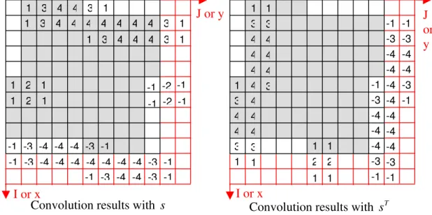
The Sobel method is a gradient method. It uses a 3x3 mask to calculate the intensity gradient of the image. The mask it uses are:

1 2 1 1 0 1 0 0 0 T 2 0 2 s and s 1 2 1 1 0 1 − ⎡ ⎤ ⎡ ⎤ ⎢ ⎥ ⎢ ⎥ =_⎢ _⎥ =_⎢ − ⎢− − − ⎥ ⎢ − ⎣ ⎦ ⎣ ⎥ ⎥⎦

e detection and , the transpose of , for vertical

sults of the Sobel edge detectors. The grey pattern represents a 10x10 binary image of a 4-sided polygon with edges not parallel to the I- and J- axis. The grey cells have values 1 and all the rest 0. The convolution result of each edge detection operation is a 12x12 sparse array. The additional elements of this array are shown in red and the values of the non-zero elements are shown.

For the horizontal edge detection, it is notable that:

T

s s

Where s is used for horizontal edg

edge detection. For an m-by-n image, the convolution result is an m+2 by n+2 array.

4 4 4 4 4 4 4 4 4 4 4 4 3 3 3 3 3 1 1 1 1 1 1 1 1 3 2 1 1 -4 -4 -4 -4 -3 -3 -1 -1 4 4

Figure 4: Convolution results of a 10x10 binary pattern with the Sobel edge detectors

Figure 4 uses a 10x10 pattern to illustrate the re

1 2 1 -4 -4 -4 -4 -4 -4 -4 -4 -4 -4 -4 -3 -4 -3 -3 -3 -3 -1 -1 -1 -1 -1 -1 -1 -3 -1 -1 -2 -2 -1 4 4 4 4 4 4 4 4 3 3 4 4 3 3 3 1 1 1 3 1 1 1 1 2 2 -4 -4 -4 -4 -4 -4 -4 -3 -1 -4 -3 -3 -3 -1 -1 -1

Convolution results with s _{Convolution results with} T

s

I or x I or x

J or y J

or y

(30)

• All cells of value greater than, or equal to 3, represent the location of the top edge

they should be ignored in the edge detection process.

• All cells of value less than or equal to -3 represent the location of the right edge ls • The bottom cell of each edge may be outside the 10x10 image frame; hence they

should be ignored in the edge detection process.

In general, the Sobel method produces thicker edges (2 cells width in our example) as or the straight line fitting. A thicker edge only means the resulting straight line will have more points to average with and its location will be slightly within the boundary of the original image. This should be an advantage.

A.5.3 Boundary polygon determination

After extracting the 4 groups of edge cells from the pattern, the remaining work is to establish the 4 boundary edges of the image. A simple least-square based curve fitting function in Matlab (polyfit) is used. The 4 boundary edges are assumed to be of the form or the horizontal lines and

(the west edge in a proper XY plane plot).

• All cells of value less than, or equal to -3, represent the location of the bottom edge (the east edge in a proper XY plane plot). However, the I values of these cells are offset by 2.

• The right-most cell of each edge may be outside the 10x10 image frame; hence For the vertical edge detection, here are some important notes:

• All cells of value greater than, or equal to 3, represent the location of the left edge (the south edge in a normal XY plane plot).

(the north edge in a normal XY plane plot). However, the J values of these cel are offset by 2.

compared with other methods, e.g. Canny. However, it is a one step method. The thicker edges do not cause a problem, because it is the points within these cells that are used f

:y=ax c+ f x=by+ for the vertical linesc 8.

Once the 4 boundary edges are found, it is simple to determine the corners,

(

x_ij y_ij

)

, of the boundary polygon by solving the intersection points of any 2 boundary edges i and j from the 4 straight line equations found:

⎫ ⎭ where i, j=1 to 4 and i ≠ j, i i ij i j j ij j a b x c a b y c ⎡ ⎤ ⎧ ⎫ ⎧ = ⎨ ⎬ ⎨ ⎬ ⎢ ⎥ ⎣ ⎦ ⎩ ⎭ ⎩ , solving 1 ij i i i x ⎫ ⎡a b ⎤ ⎧ ⎫c = ⎨ ⎬ ⎢ ⎥ ⎨ ⎬ − ⎧

(31)

A.5.4 Contour polygon calculation with constant scale factor

From section A.1.2, it is found that the surface interpolation of the point cloud image will lts introduce edge effects. An inner contour polygon is required to filter out erroneous resu from the image delta. To determine the vertices of this inner polygon, one can use the following calculations.

(

)

1 1 P′= x′ y₁′

(

)

1 1 1 P = x y 1 P 1 P′ 1 y −y 1 y′ −y P

(

)

P= x y

Take any point within the polygon, e.g. the centroid P , then

(

)

1 4

(

)

4 i i i P= x y =

∑

x y If i i PP PP α ′

= , the scale factor, then

1 1 i i x x y y x x y y α ′− ′− = = − − , giving

(

1

)

i i x x x i i y α y α y ′ ⎛ ⎞₌ ⎛ ⎞_{+ −} ⎛ ⎞ ⎜ ⎟ ⎜ ⎟ _{⎜ ⎟}, for i=1 to 4. ′ _{⎝ ⎠} ⎝ ⎠ ⎝ ⎠

The following figure shows the boundary polygon obtained for the exposed surface of sample A with α =0.1

(32)

The following figure shows the boundary polygon obtained for the exposed surface of mple B with

(33)

(34)

(35)

B.1 Matlab Code

he Matlab code main6 contains the common code for the image processing and orrosion volume calculation for each corroded sample. The operator is expected to

odify the front portion of the code to point to the input and output file directories and e file names required.

.1.1 Sample A

imulated Corrosion Depth 0.08 mm

T c m th B S nction main6

This function calculates the depth of erosion of a buried sample by calculating the image difference of the original surface and the eroded surface after some time of burial.

This function carries the following steps: Notes:

1. All image files are cloud point files. The positions of the cloud are represented in the file as 3 columnes of numbers corresponding to the x, y and z values of the points respectively. The numbers are represented in ASCII form with 6 places of decimals. This is the format that PolyWork use to output the point clouds.

istory:

008-09-09 created from main5_part1 and main5_part2 008-09-22 remove sub-function format

008-09-23 in find_image_boundaries, polyfit will fail when the resulting line is close to verticle. Need to reverse x and y to get a % proper fit

%20 %20 %

% 2. add dynamic range for displaying ed_2D

%2008-10-15 Use outside and inside polygons for croping and result % interpretation respectively to

% 1. cut down edge distortion introduced by surface interpolation % 2. avoid including portion of the protected surface due to the % non-planar nature of the corroded surface making the

% surface normal only a rough estimation.

%2008-10-16 Modify main & rotate_image to crop the rotated Imo using the % polygon instead of Imo_exp. This is more correct.

clear all; close all;

% Program parameters setup section

% Input files

fpath = ['..' filesep '..' filesep]; %file directories common path

fpathi1 = [fpath 'Take 4' filesep]; %input file directory for original sample

fpathi2 = [fpath 'Take 4 modZ-0.08' filesep]; %input file directory for eroded sample

%The original image of the sample before erosion

fn_imo = [fpathi1 '200808111515 Sample A - Point Cloud - Take 4.txt'];

%The exposed area of the original surface

fn_imo_exp = [fpathi1 '200809241146 Take 4 Step 2 - Exposed.txt'];

%The image of the sample after erosion

fn_ime = [fpathi2 '200809241503 EST 0.08 Step 1 - Start Pos.txt'];

%The image of the sample after erosion with eroded part cut off

fn_imeh = [fpathi2 '200809241510 EST 0.08 Step 2.txt'];

%The aligned image of the eroded sample with eroded part cut off

fn_imeha = [fpathi2 '200809241548 EST 0.08 Step 3 - After.txt'];

%Output files for display and validation

fpatho = [fpath 'Take 4 modZ-0.08' filesep]; %output file directory

fu % % % % % % % % % % % %H %2 %2 %2 %

08-09-26 add polygon area calculation

08-10-01 1. change the accuracy of erosion volume calculation to improve its accuracy.

(36)

today=datestr(date,26); fpathod = [fpatho today

%The full eroded image

today=today(find(today~='/')); %remove '/' from today

' ']; %output file directory + today aligned with the original image

s

%The resolution required for edge detection: scan line spacing distance

% distance in mm

r the image processing

RESOLUTION = 0.05; % distance in mm

am

ead_image(fn_imeh);

form Ime so that it will align with Imo

axis

(Imo_exp,Imo,Imea);

ded polygon. Two nd the

n_imo_exp_r,Imo_exp_r); n_ime_exp_r,Ime_exp_r);

sion and display results

,RESOLUTION,poly_in); %the erosion distribution

ON,poly_in); fn_imea = [fpathod 'EST 0.08 Step 4.txt'];

%The eroded exposed surface after rotation to align the surface normal with z-axi

fn_ime_exp_r = [fpathod 'EST 0.08 Step 4-Exp R.txt'];

%The original exposed surface after rotation and cropped

fn_imo_exp_r = [fpathod 'EST Take 4 Step 4-Exp R.txt']; S_LINE_DIST = 0.2; %The resolution fo % main progr

% read all images

Imo=read_image(fn_imo); Ime=read_image(fn_ime); Imeh=r Imeha=read_image(fn_imeha); Imo_exp=read_image(fn_imo_exp);

% Calculate the transformation matrix to apply to Imeh to get Imeha

% Note: The transformation must be a 3x3 matrix

T=Imeh\Imeha;

% Trans

Imea=Ime*T;

% Save image to file for display

save_image(fn_imea,Imea);

o that their surface normal are parallel to the

%Orientate images s

[Imo_exp_r,Imo_r,Imea_r]=rotate_images

he original exposed surface projected onto

% Find the boundaries of t

% the XY plane. The boundaries are defined as a 4-si

% polygons are determined. The outer one is for image cropping a

filtering.

% inside one is for image delta results

[poly_out,poly_in]=find_image_boundaries(Imo_exp_r,S_LINE_DIST);

% Use the polygons to isolate the image area of the original exposed

% surface and the eroded sample for erosion depth calculation

Imo_exp_r=crop_image(Imo_r,poly_out); Ime_exp_r=crop_image(Imea_r,poly_out);

% Save all files for validation

save_image(f save_image(f

% Calculate the degree of ero

ed2D=image_delta(Imo_exp_r,Ime_exp_r in 2D s(ed2D,RESOLUTI display_result return %---% Helper Functions

(37)

%This function calculates the z-distance delta of im1 and im2 and

%im1 is considered as the reference image.

%res is the resolution of the grid

%poly is the polygon which is the boundary for valid results

%Method: It fits a surface each to im1 and im2 and project a grid

ints to

%at resolution res on both surfaces and use the grid po

%sample the surfaces for delta. At the end, it filters out all results

]); es + 1); min)/res + 1); images in); grid 1=im1(:,3); im2(:,3); Ygrid,'cubic'); d,'cubic'); - Gim2(1:y_size,1:x_size); im2,im3)

of this plane is pointing in the

re method.

s (A,B,C)

ne_Unit_Norm=ABCD(1:3)/norm(ABCD(1:3));

it_Norm

xis));

the plane formed by the z_axis and

;

otation matrix

c=RU_axis(3);

%outside the polygon given.

% find bounding box and grid for the data

xyzmin=min([im1;im2]);xyzmax=max([im1;im2 xmin=xyzmin(1);ymin=xyzmin(2); xmax=xyzmax(1);ymax=xyzmax(2); xmin)/r ylin=linspace(ymin,ymax,(ymax-y

% setup a common grid for both

grid(xlin,yl [Xgrid,Ygrid]=mesh

% fit the image into the

X1=im1(:,1);Y1=im1(:,2);Z X2=im2(:,1);Y2=im2(:,2);Z2= Gim1=griddata(X1,Y1,Z1,Xgrid, Gim2=griddata(X2,Y2,Z2,Xgrid,Ygri

% find the difference with the common parts of the two images

[y_size1,x_size1] = size(Gim1); [y_size2,x_size2] = size(Gim2); x_size = min([x_size1, x_size2]); y_size = min([y_size1, y_size2]); im_diff = Gim1(1:y_size,1:x_size)

% filter out results outside the polygon

% convert polygon into integer indices into im_diff

+1; polyIJ=round((poly - ones(size(poly,1),1)*[xmin ymin])/res)

generate all the indices of im_diff

%

[XI,YI]=meshgrid(1:x_size,1:y_size);XI=XI(:);YI=YI(:);

% find all indices inside or on the polygon

[IN,ON]=inpolygon(XI,YI,polyIJ(:,1),polyIJ(:,2)); OUT=~(IN | ON); % all indices outside the polygon

% delete all results outside the polygon

im_diff(sub2ind(size(im_diff),YI(OUT),XI(OUT)))=NaN; return

function [im1r,im2r,im3r]=rotate_images(im1,

%This function finds the plane that best fits im1 and rotate both

%im1, im2 and im3 so that the normal

%z-axis.

%Find the 3D plane that best fits im1 using least squa

%The plane is defined as Ax+By+Cz+D=0 that passes through im1,

ABCD=fit_plane(im1);

%Calculate the axis of rotation

normal vector to plane Ax+By+Cz+D=0 i

%The

Pla

%Angle between Z axis and Plane_Un

z_axis=[0,0,1]';

theta=acos(dot(Plane_Unit_Norm,z_a

%Rotation axis is normal to

%Plane_Unit_Norm

R_axis=cross(Plane_Unit_Norm,z_axis)

s/norm(R_axis); %unit vector of R_axis

RU_axis=R_axi ate the r %Cre a=RU_axis(1);b=RU_axis(2); sym=RU_axis*RU_axis';skew=[0,-c,b;c,0,-a;-b,a,0]; Xform=sym*(1-cos(theta))+skew*sin(theta)+eye(3)*cos(theta); m=Xform'; %rotate the matrix to suit our image format

Xfor

(38)

im1r=im1*Xform; im2r=im2*Xform; im3r=im3*Xform; %debug code de

display(['Before orientation, theta = ',num2str(theta*180/pi),' gree']);

r(phi*180/pi),' degree']);

oint of cloud using the equation

problem to find the a's. A=P'*Z we can solve A.

the point cloud image

nd_image_boundaries(im,res)

olygon containing im on the XY n the XY plane has to be bounded

to d or ines. e effects. n=min(im_XY);xymax=max(im_XY); l operator

horizontal and vertical edges are ref to the XY plane

abcd=fit_plane(im1r);

; PUN=abcd(1:3)/norm(abcd(1:3)) phi=acos(dot(PUN,z_axis));

display(['After orientation, theta = ',num2st return

function plane=fit_plane(im)

%This function fits a plane through the image p

%least square method. The plane is desribed by

%z=a0+a1x+a2y. plane=[-a1 -a2 1 -a0]'

%Method:

n

%This is a multiple linear regressio

%If P=[ones X Y] and A=[a0 a1 a2]', then the least square error

%of plane A will occur at P'*P*

n=size(im,1); %n=number of points in

P=[ones(n,1) im(:,1) im(:,2)]; A=(P'*P)\(P'*im(:,3));

plane=[-A(2);-A(3);1;-A(1)]; return

function [polygon_out, polygon_in]=fi

%This function finds the 4-sided p

%plane. The projected image of im o

%by 4 straigth lines. res is the resolution required for this

%operation. res has to be large enough so that when we fit im

ttern will have soli

%the grid formed by res, the resulting pa

%edges in most of the places.

%This funciton creats an XY grid using res and fits the XY

%projections of im into this grid. It uses the Sobel edge operat

lines through the edge

%to detect the 4 edges. It then fits 4

%points of im and returns the intersections of these 4 l

t down edg

% 20081014: The polygon is shrunk by 5% to cu

% project im onto the XY plane

im_XY=im(:,1:2);

% fit the project image points into a grid

xymi

dim=uint32(ceil((xymax-xymin)/res))+1; %dim=MxN of the grid

% calculate the(i,j)cell each point of im_XY to fit into the grid

im_IJ=uint32(floor((im_XY-ones(size(im_XY,1),1)*xymin)/res))+1; %index starts from 1

2ind(dim,im_IJ(:,1),im_IJ(:,2)); im_ind=sub

% fit into the grid

grid=zeros(dim); grid(im_ind)=1;

% Detect the 4 edges in the grid

s=[1 2 1;0 0 0;-1 -2 -1]; %Sobe

H=conv2(grid,s);V=conv2(grid,s'); % H&V markes the

for i=1:4

switch i % north, east, south & west

case 1 % west edge detection

(39)

% ensure J will not be > dim(2) ind(J<=dim(2)-3);I=I(idx);J=J(idx); ]=find(V>3); to this edge switch i if j>4

out(:,1),polygon_out(:,2),'r-mi that is within the the XY plane. age ed output image on o(:,2),'b.'); g forms: epth depth n idx=f

case 4 % south edge detection

[I,J

% ensure I will not be be greater than dim(1)

idx=find(I<=dim(1)-3);I=I(idx);J=J(idx); end

% find all points belonging

pts=im_XY(ismember(im_IJ,[I,J],'rows'),:); % fit a straight line through these points

case {1,3} %east & west edge

%reverse x and y to get better fit

line=polyfit(pts(:,2),pts(:,1),1); edge(i,:)=[1 -line(1) line(2)]; case {2,4} %north & south edge

line=polyfit(pts(:,1),pts(:,2),1); edge(i,:)=[-line(1) 1 line(2)]; end

end

is boundary

% find the 4 corner points of th

for i=1:4 j=i+1; j=1; end a=[edge(i,1);edge(j,1)]; b=[edge(i,2);edge(j,2)]; c=[edge(i,3);edge(j,3)]; polygon_out(i,:)=[a b]\c; end

% shrink the polygon by 10%

xymean=ones(size(polygon_out,1),1)*mean(polygon_out);r=0.1; polygon_in=xymean*r+polygon_out*(1-r);

% close the polygons

polygon_out=[polygon_out;polygon_out(1,:)]; polygon_in=[polygon_in;polygon_in(1,:)]; % debug code % figure;plot(im(:,1),im(:,2),'b.',polygon_ o',polygon_in(:,1),polygon_in(:,2),'r-o');

% xlabel('x axis (mm)');ylabel('y axis (mm)');

% title('Derived boundaries of the exposed sample surface');

return

function imo=crop_image(imi,polygon)

%This function returns all the points from i

e polygon has to be on

%polygon supplied. Th

im

%imi is the input

%imo is the cropp

% find the XY projection of imi

X=imi(:,1);Y=imi(:,2);

% setup the polygon

:,1);pY=polygon(:,2); pX=polygon(

% find all the points inside the polygon

[IN,ON]=inpolygon(X,Y,pX,pY);

% find all the image points within the polyg

imo=imi(IN|ON,:); % % debug code % figure; % plot(polygon(:,1),polygon(:,2),'-ro',imo(:,1),im return function display_results(ed_2D,res,polygon) owin

% This function displays the erosion depth in the foll

erosion depth

% 1. 2D image with color coding the

osion d

% 2. the histogram of the er

% 3. the statistical distribution of the erosion

polygon for erosion calculatio

Measuring corrosion levels of ductile iron pipes using scanned images

NRC Publications Archive

Archives des publications du CNRC

M e a suring c orrosion leve ls of

duc t ile iron pipe s using

sc a nne d im a ge s

R R - 2 6 8

N o v e m b e r 2 0 0 8

Executive Summary

Table of Contents

1 Background

1.1 The Project

1.3 The Technology & Challenges

2 The Proposed Process

STEP 1

STEP 2

STEP 1

STEP 2

STEP 3

STEP 4

STEP 5

3 Test Results

3.1 Sample A

3.2 Sample B

4 Discussion

5 Future Improvements

6 Conclusion

A.1 Image delta of two point cloud data sets

A.2 Corrosion Volume and Mean Depth Calculation

∑

∑

A.3 Fitting a plane to the image

(

)

(

)

(

)

(

)

(

)

∑

∑

(

)

∑

(

)

(

)

∑

∑

∑

∑

∑

∑

∑

∑

∑

∑

∑

∑

∑

[ ]

[ ]

{ }

{ }

[

] [ ]

{ }

[ ]

{ }

{ }

{ }

(

[ ] [ ]

)

(

[ ]