Assessing computational methods and science policy in systems biology

Assessing Computational Methods and Science

Policy

in

Systems Biology

OFTECHNOLOGY

by

_{JUN 3 0 2009}

Andrea R. Castillo

LIBRARIES

B.S. Electrical Engineering and Computer Engineering,

Minor Computer Science

Carnegie Mellon University 2005

Submitted to the Engineering Systems Division

in partial fulfillment of the requirements for the degree of

Master of Science in Technology and Policy

at the

MASSACHUSETTS INSTITUTE OF TECHNOLOGY

June 2009

@2009 Massachusetts Institute of Technology. All rights reserved.

Author ...

Engineering Systems Division

_

,/Iay 8, 2009

C ertified by ...

Bruce Tidor

Professor of Biological Engineering and Computer Science

Thesis Supervisor

Accepted by ...

....

Dava Newman

Professor, Aeronautics and Astronautics and Engineering Systems

Director, Technology and Policy Program

Assessing Computational Methods and Science Policy in

Systems Biology

by

Andrea R. Castillo

Submitted to the Engineering Systems Division on May 8, 2009, in partial fulfillment of the

requirements for the degree of Master of Science in Technology and Policy

Abstract

In this thesis, I discuss the development of systems biology and issues in the pro-gression of this science discipline. Traditional molecular biology has been driven by reductionism with the belief that breaking down a biological system into the funda-mental biomolecular components will elucidate such phenomena. We have reached limitations with this approach due to the complex and dynamical nature of life and our inability to intuit biological behavior from a modular perspective [37].

Mathematical modeling has been integral to current system biology endeavors since detailed analysis would be invasive if performed on humans experimentally or in clin-ical trials [17]. The interspecies commonalities in systemic properties and molecular mechanisms suggests that certain behaviors transcend specie differentiation and there-fore easily lend to generalizing from simpler organisms to more complex organisms such as humans [7, 17].

Current methodologies in mathematical modeling and analysis have been diverse and numerous, with no standardization to progress the discipline in a collaborative man-ner. Without collaboration during this formative period, successful development and application of systems biology for societal welfare may be at risk. Furthermore, such collaboration has to be standardized in a fundamental approach to discover generic principles, in the manner of preceding long-standing science disciplines.

This study effectively implements and analyzes a mathematical model of a three-protein biochemical network, the Synechococcus elongatus circadian clock. I use mass action theory expressed in kronecker products to exploit the ability to apply numer-ical methods-including sensitivity analysis via boundary value formulation (BVP) and trapiezoidal integration rule-and experimental techniques-including partial re-action fitting and enzyme-driven activations-when mathematically modeling large-scale biochemical networks. Amidst other applicable methodologies, my approach is grounded in the law of mass action because it is based in experimental data and

biomolecular mechanistic properties, yet provides predictive power in the complete delineation of the biological system dynamics for all future time points.

The results of my research demonstrate the holistic approach that mass action method-ologies have in determining emergent properties of biological systems. I further stress the necessity to enforce collaboration and standardization in future policymaking, with reconsiderations on current stakeholder incentive to redirect academia and in-dustry focus from new molecular entities to interests in holistic understanding of the complexities and dynamics of life entities. Such redirection away from reductionism could further progress basic and applied scientific research to embetter our circum-stances through new treatments and preventive measures for health, and development of new strains and disease control in agriculture and ecology [13].

Thesis Supervisor: Bruce Tidor

Acknowledgments

This study was fulfilled due to the collaborations and contributions of A. Katharina Wilkins, Jared E. Toettcher, and Jacob K. White. I am especially grateful to my thesis supervisor, Bruce Tidor, for his invaluable perspective, direction, and support.

Contents

1 Introduction 15

1.1 Systems Biology Overview ... ... . 15

1.2 Significance of this Study ... ... 17

2 Background 19 2.1 Current Methods ... ... 19

2.2 Contributions ... ... .. 20

3 Analysis of the Autonomic Protein Oscillation from Synechococcus elongatus 25 3.1 Introduction ... ... 25 4 Methods 29 4.1 Model Structure ... ... . 29 4.2 Parameterization . ... ... 32 4.3 Sensitivity Analysis ... ... 34

5 Results and Discussion 39 6 Conclusions and Recommendations 55 6.1 Summary of Findings ... ... 55

6.2 Policy Issues ... ... .. 55

6.3 Policymaking ... ... 57

A Supplemental Information (SI) 63

List of Figures

5-1 Model Verification. Mass action modeling dynamics overlayed with the original Rust et al. dynamics. (A) The original Hill-Langmuir model and our mass action model trajectories overlaid. Total KaiC accounts for the total amount of phosphorylated KaiC, excluding U-KaiC (unphosphorylated): D-U-KaiC (doubly phosphorylated on serine 431 and threonine 432), S-KaiC (serine 431 phosphorylated), and T-KaiC (threonine 432 phosphorylated). Experimental data (solid sym-bols) for phosphorylation (B-C) and dephosphorylation (D) kinetics was used by Rust et al. to fit their model (hollow symbols). ... 40 5-2 Abstracted Visual Representation of the Mass Action Model.

Here is an abstraction of our mass action model where arrow thick-nesses represent reaction rates that are weighted logarithmically ac-cording to magnitude where the thickest arrows represent the fastest kinetics. The reaction rates are approximately: > 1 (thick arrow),

> 0.1 (medium arrow), < 0.1 (thin arrow) . . ... 42

5-3 Time Course Trajectories of Species Concentrations. Here we plot the trajectories of the species (state variables) that occur at ap-preciable concentrations. The presence or absence of free KaiA in the model drives two regimes of behavior, Phase I and Phase II, within the circadian period. During autokinase (Phase II), unactivated S-KaiC binds to KaiB and sequesters free KaiA to form the KaiABC complex, as shown by the magenta trajectory. Furthermore, all free KaiA in the

5-4 Scaled Period Sensitivities .log Period sensitivities are imposed on this abstracted visual representation of the mass action model. The arrow thicknesses represent period sensitivities that are weighted log-arithmically according to the highest magnitude where red is positive sensitivity and green is negative sensitivity. The period sensitivity magnitudes are approximately: > 1 (thick arrow), > 0.1 (medium

arrow), < 0.1 (thin black arrow). ... . . . . . . . . . 44

5-5 Circadian Period Decomposition. The mass action model was de-composed into a dephosphorylation interval (B) and a phosphorylation interval (C) by implementing enzyme-driven switch-like behavior (D). (A) The superimposition of Phases I (B) and II (C) results in the full

trajectories of the mass action model. ... . . . . 45

5-6 Scaled Period Sensitivities l for the Decomposed Period. The dephosphorylation (left) and phosphorylation (right) intervals of a circadian period is shown here. The transition from unactivated S-KaiC to unactivated U-KaiC plays the most significant role in set-ting the period during KaiC dephosphorylation. Conversely, an ar-ray of kinetics influence the periodicity during KaiC phosphorylation. The arrow thicknesses and colors represent period sensitivities that are weighted logarithmically according to the same spread for period

5-7 Flux Pathways for the Phosphoform Interconversion during the Full and Decomposed Period. The phosphoform flux

distri-bution is shown here for a full period along with the flux distridistri-bution for the desphosphorylation interval (bottom, left) and phosphorylation interval (bottom, right) for the same period. The majority of the flux distribution occurs during the phosphorylation interval, specifically from activated U-KaiC to activated T-KaiC. The arrow thicknesses represent the overall flux for each time course according to the highest magnitude, where the magnitudes are approximately: > 4 (thick blue arrow), 4 > ( > 1 (medium blue arrow), 2 0.1 (thin blue arrow), < 0.1 (thin black arrow). Not graphed here are the fluxes orthogonal to the phosphoform interconversion planes, on account of these reaction rates being invariably parameterized on a faster time-scale. ... . 48 5-8 Scaled Angular Peak-to-Peak Phase Sensitivities '. The phase

sensitivities are weighted logarithmically according to the same spread for period sensitivities in Figure 5-4. The peak-to-peak analysis was computed for sequential peaks starting from in between the dephos-phorylation and phosdephos-phorylation intervals of the period, when U-KaiC is at a maximum. These phase sensitivities are diametric depending on which peak is ordered first, such that the D-KaiC to T-KaiC phase sensitivities has the same magnitude as the T-KaiC to D-KaiC phase sensitivities but with an opposite sign. . ... 50 5-9 Minimal Oscillating Networks. A collection of minimalized

oscil-lating networks from the original mass action model were discovered. In (A) and (C) we illustrate the two most minimalized networks we found, with the corresponding oscillatory dynamics shown in (B) and (D) respectively. These diagrams show distinct sequences of phospho-form interconversion. The arrow thicknesses and colors in (A) and (C) represent period sensitivities that are weighted logarithmically accord-ing to the same spread for period sensitivities in Figure 5-4. ... 52

A-1 Full Graphical Description of the Mass Action Model. (I) The model accounts for time-varying biochemical concentrations (state variables) of heteromultimeric complexes formed by the Kai proteins,

along with the intermediate protein complexes, such as Michaelis com-plexes, within the autokinase and autophosphatase reactions of KaiC that maintain oscillation. (II) The reactions described here show the

affect of KaiA allosteric regulation on KaiC activation, where the KaiA-bound KaiC form is the transition state from unactivated to activated KaiC. (III and IV) KaiABC complex assembly (III.b) and disassembly (III.a and IV) are accounted for by combinatorial intermediate bind-ing states. The general principles are that (1) KaiB and KaiA can only assemble with the S-KaiC phosphoform, (2) KaiB can only dis-assemble from the D-KaiC, T-KaiC, and U-KaiC phosphoforms, and (3) KaiA may disassemble from any of the phosphoforms. A MATLAB implementation of the mathematical model is provided in the following

appendix . ... .. ... 66

A-2 Scaled Absolute (left) and Scaled Relative (right) Amplitude Sensitivities 0 . The amplitude sensitivities are weighted logarith-mically according to the same spread for period sensitivities in Figure 5-4. The absolute amplitude of a species is the concentration level and the relative amplitude is the difference between its maximum and minimum concentrations, where the concentration is periodic in time. 68

List of Tables

A.1 The assembly and disassembly reactions are shown here. The corre-sponding reaction rates are in Table A.5 and a graphical representation of the corresponding pathways is shown in Figures A-1(III) and A-1(IV). 69 A.2 The KaiA allosteric regulation reactions are shown here. The

corre-sponding reaction rates are in Table A.6 and a graphical representation of the corresponding pathways is shown in Figures A-1(II). ... 70 A.3 The KaiC phosphoform interconversions at basal rates are shown here.

The corresponding reaction rates are in Table A.7 and a graphical representation of the corresponding pathways is shown in Figure A-1(I). 71 A.4 The KaiC phosphoform interconversions with maximal effect of free

KaiA are shown here. The corresponding reaction rates are in Table A.8 and a graphical representation of the corresponding pathways is

shown in Figure A-1(I) .. . . . . ... ... 72

A.5 The KaiABC assembly and disassembly occur at a much more rapid time scale in comparison to the KaiC phophoform interconversions. . 73

A.6 The KaiA allosteric regulation occurs at a much more rapid time scale in comparison to the KaiC phophoform interconversions and is at most

an order of magnitude slower than KaiABC complexing. . ... 74

A.7 The KaiC phosphoform interconversions at the basal rate autodephos-phorylate due to the absence of free KaiA. Due to the role that free KaiA plays in allosterically regulating KaiC phosphoform

A.8 The KaiC phosphoform interconversions with maximal effect of free KaiA. Serine dephosphorylation does not occur due to the role that S-KaiC plays in sequestering free KaiA from the system. . ... 76 A.9 The initial concentrations of six of the state variables are provided

here. The remainder of the 75 total state variables are initialized to zero. 77 A.10 The 75 state variables are listed here along with the mass conservation

relationships to the total amounts of KaiA, KaiB, and KaiC for this

post-translational oscillator. ... . . . 80

A.11 This control matrix captures the outputs of interest which are the four KaiC phosphoforms: serine and threonine phosphorylated KaiC (D-KaiC), serine phosphorylated KaiC (S-KaiC), threonine phospho-rylated KaiC (T-KaiC), and unphosphophospho-rylated KaiC (U-KaiC). Al-ternative control matrices could be implemented to capture KaiABC

complexing levels and any other outputs of interest. . ... 83

A.12 These reactions implement an enzyme-driven switch-like behavior. This rapid process corresponds to the computational experiment in Figure

5-5 and the results in Figures 5-6 and 5-7. . ... 84

A.13 These are the reaction rates for the enzyme cascade specified in the above table, Table A.12. . . ... ... 85

Chapter 1

Introduction

1.1

Systems Biology Overview

Modern biology explains living beings to be highly organized and complex material entities composed fundamentally of molecules due to a long process of evolution and replication [10]. Life is one of the most complex phenomena known in the universe [26]. Systems biology is an integrative study of life by (1) investigating cellular com-ponents and molecular interactions, (2) applying experimental and computational techniques, and (3) analyzing complex interactions to discover new emergent proper-ties that may arise from a systematic and holistic paradigm. Systems biology draws upon all areas of biology and natural science [8] to quantitatively assess the dynamic interactions between several entities of a biological system [9]. In traditional molecu-lar biology, there has been a certain tradition in the reductionist method of dissecting biological systems into their constituent entities as an effective way to explain biolog-ical processes. Limitations in this approach are that biologbiolog-ical systems are extremely complex and dynamical, having emergent behaviors that are nonintuitive and unex-plainable by studying their constituent entities alone [37]. Therefore, systems biology aims to understand emergent behaviors of the system holistically as opposed to the constituent entities singularly [9].

origin and methodological foundations for systems biology (1) in the accumulation of detailed knowledge with the prospect to advance current practices in biotechnology and health care, (2) in the emergence of new experimental techniques and framework design, (3) in mathematical modeling principled in controls theory, systems theory, and current biological understanding, (4) in the development of computational meth-ods to address high-throughput and resource-intensive analysis, and (5) in the internet as the medium for quick and comprehensive exchange of information [26].

Systems biology is driven by curiosity of scientists and engineers, but even more so by the prospect of its applications to predict the outcome of complex processes. Currently the discipline is still in its formative period, lacking a systematic approach to modeling biochemical networks and signaling pathways in such a way that es-tablishes experimentally testable quantitative predictions despite the complex nature of systems biology models, not to mention the complexity of the underlying biol-ogy. The synthesizing of experimentation with theory in systems biology models has been a modus vivendi to the discipline. A principled and fundamental approach to the experimentation, mathematical modeling, and quantification is crucial for further successful development of biological science [26].

Systems biology, a new mathematical and computational science, has the joint ob-jectives of reducing experimental and clinical treatment costs, and rapidly advancing current knowledge of biological systems [3]. The integrative approach of systems bi-ology provides 'sufficiently accurate and detailed' models which allow biologists to accomplish the following tasks not possible by traditional biology research: predic-tion of biological system behavior given an perturbapredic-tion and knock-out or redesign of biochemical networks to create completely new nonintuitive emergent biological system properties [1]. Being that systems biology lacks a foundational and system-atic approach across wet- and dry-labs, current collaborative efforts to progress the discipline have been demanding, and thus matching investment into new theoretical methods is required.

1.2

Significance of this Study

Standardization of systems biology principles can lead to practical use in a comple-mentary technology, synthetic biology, which is to design new and improved biological functions [4]. There are significant implications of this synergy for health (through development of new treatments and new preventive measures), and agriculture and ecology (through development of new strains and disease controls) [13].

In order to better understand biological systems, perturbation of these systems en-ables us to analyze how emergent behaviors occur. Such analysis cannot be easily or ethically performed on humans experimentally; thus, model organisms provide the approach of choice [17]. The Human Genome and prior studies have inspired current efforts in biology by the observation that different species have many systemic prop-erties and molecular mechanisms in common. This might be the result of ancestral relationships and evolutionary dynamics of life in all living organisms due to simi-larities in genetic code, metabolic and pathways, molecular machinery. Interspecies commonalities suggest that all life arose from a single common ancestor and leads to predictive power in the fundamental understanding of biological systems that tran-scends specie differentiation [7, 17]. Thus it is a common practice to generalize from the simpler organisms to more complex organisms such as humans [17].

Chapter 2

Background

2.1

Current Methods

The practical application of computational simulation to systems biology has transi-tioned biology and related applied research away from being purely descriptive science to being a predictive science [18]. Such modeling is most useful when it (1) produces useful predictions, (2) matches experimental results, (3) generates data at a granu-larity beyond present-day experimental capabilities, (4) yield nonintuitive insights of the system behavior, (5) identify uncertain components, functions or processes in a system, and (5) perform computational experiments to save time, cost, and effort [27].

Besides the enormous challenge for integrating different levels of information pertain-ing to genes, mRNAs, proteins, and pathways, a more immediate and fundamental barrier to systems biology progress is in defining a principle approach to modeling methodologies, in developing powerful analyses, and in integrating this information into experimental strategies in order to make discoveries [18]. In contrast to long-standing engineering disciplines, there is a relative inadequacy of software and meth-ods currently available and standardized for analyzing biological circuits. The multi-tude and diversity of approaches to computational simulation is extensive, including ordinary differential equations, stochastic differential equations, partial differential equations, power law equations, petri nets, cellular automata, and agent-based

mod-els [27].

Systems biology is a science; as a science, it should aim to discover generic prin-ciples [7]. _{System-level understanding necessitates a foundation of principles and} methodologies that couple molecular mechanism to biological system behavior [25].

Considering an appropriate level of complexity between abstraction and detail, math-ematical models should be designed to synthesize and transform information into in-sight.

Experts in the field have stressed the necessity for widespread standard notation of theoretical frameworks and tools for integrating information, displaying models graphically, and mathematical modeling and simulation of biological system. The integration of technology, biology, and computation is a commanding challenge to basic and applied systems biology research, for both academia and industry. Such an initiative towards standardization would enable studies at different institutions to directly exchange their fully detailed mathematical models [18].

2.2

Contributions

The progress and societal contributions of systems biology depend decisively on the collaborative development of modeling complex systems [9]. A major motivation of current work is the analysis of biochemical networks including gene networks, pro-tein interaction networks, metabolic networks, and signaling networks. The presence of biological uncertainties have driven researchers to study more realistic and de-tailed models in order to understand these biological phenomenas. Currently there is no standard formulation for these biochemical networks, and therefore an array of mathematical modeling techniques and analytical methods have been implemented in attempt to figure out what works. In this study we propose a formulation of a

three-protein interaction network, the Synechococcus elongatus circadian clock, using mass action theory expressed in kronecker products. Such formulation may exploit the simple algebraic manipulation of large-scale biochemical networks and serve as a basis for efficient and general application of methods [5, 12].

The understanding of the structural-functional relationships of molecules have evolved due to the capability of quantifying the law of mass action dynamics in systems bi-ology models [43]. The law of mass action, introduced by Guldberg and Waage in the nineteenth century, is a powerful and well-established concept that descibes the average behavior of a dynamical and complex system. Specifically it states that the rate of a reaction is proportional to the probability of interaction of the reactants. This probability, in turn, is proportional to the concentrations of the reactants to the stochiometry, the power of the molecularity. Implicit in the 'proportionality' aspect of this Law is an assumption that the quantities concerned in inducing inter-actions and transitions are in a homogeneous solution. The phenomenology of this Law can, in principle, be derived from statistical mechanics and quantum mechanics, although it is regarded as accurate due to the wealth of experimental information on a varity of biological, chemical and physical science based theories that assume it [41].

This approach incorporates structural and biophysical properties of the constituent molecules by modeling the resulting molecular mechanism. Therefore, given knowl-edge of initial species concentrations, which is an entity of one or more molecules, and parameterization of how these molecules interact, the law of mass action provides a complete delineation of the biological system dynamics at all future time points. We denote the concentration of the reactants by lower case letters

where the concentration is traditionally denoted in the brackets. The biological sys-tem dynamics is represented schematically by

S + E S : E k~- P + E.

k-_1

where the reactions occur at an associate rate parameter constant, in this case kl, k_₁

or k_{2, and the double-stacked arrows indicate a reversible reaction and the single arrow} an irreversible reaction. The example mechanism provided here is the conversion of a substrate S, by catalysis of an enzyme E, _{into a product P. The stochiometry of}

this system is one, where one molecule of S combines with one molecule of E to form a two molecule S : E _{complex, which eventually produces one molecule of P and one}

molecule of E. _{The law of mass action, applied to the above set of reactions leads to}

an equation per each reactant, and hence the system of ordinary differential equation (ODE) system for nonlinear reactions as follows

d[S] dt = -k1 i [E] [S] + (k_1 k2) [S: E], dt d[S : E] dt = ki -[E] -[S] - (k_1 + k2) [S : E], d [P] and dP k2 [S : E]. dt

The reaction rate constants, represented as the k's, are the constants of proportion-ality in the application of the law of mass action [30]. To implement a time series simulation, the initial conditions, which are those at the start of the process which converts S to P, _{must be set for the concentration of the reactants.}

To efficiently simulate an example biochemical network and compute numerical meth-ods on nonlinear ODE models, I have implemented mass action kinetic modeling in Kronecker product formulation [5] to assess principle methods of mass action model-ing and analysis in systems biology. Emphasis was placed on assessmodel-ing the objectivity

of this approach and how this approach affects interpretation and definition of the biochemical network behavior. From a scientific perspective, the goal was to deter-mine emergent properties of the system utilizing the mathematical modeling proposed here. Although the mathematical modeling is part of an iterative model design cy-cle including feedback from proposed experimental frameworks [9], this study was an effort to determine the advantage of grounding systems biology approaches in the foundational theory of mass action dynamics and computational representation in the Kronecker product.

Chapter 3

Analysis of the Autonomic Protein

Oscillation from Synechococcus

elongatus

3.1

Introduction

The oscillation of KaiC phosphorylation patterns in the cyanobacterium Synechococ-cus elongatus is responsible for the maintenance of stable circadian rhythms in this organism [19, 22, 23]. Here we have undertaken a computational approach to under-stand better this complex biological network.

Mathematical models are emerging as useful tools for representing and testing our understanding of complex biological systems of a variety of scales. In particular mech-anistically detailed models are being developed to capture the underlying structure, dynamics, and detailed mechanisms of biochemical networks. Such models are able to account for complex biological phenomena by representing simple kinetic relation-ships that are readily simulated and analyzed.

of multiple modification states and complexes formed. In this study we use a mass action approach for analyzing the relationship between network topology and ki-netic behavior in the in vitro circadian clock of the freshwater cyanobacterium, S.

elongatus. The cyanobacterial circadian clock enables S. elongatus to adapt cellular

performance to daily changes in the environment and provides a daily rhythm to photosynthetic regulation [16, 15]. Kondo et al. has shown that circadian oscillations can be reconstituted in vitro using only three proteins: KaiA, KaiB, and KaiC [31]. KaiC phsophorylation oscillates with the circadian period. Although it is known that KaiC phosphorylation oscillates with a circadian period, the fundamental mechanism and a clear understanding of the dynamics is indeterminate. Understanding such complexity may be advanced through mathematical modeling.

The cyanobacterial circadian clock is an ideal candidate to assess methodology due to the stable KaiC phosphorylation cycle in vitro as an expected emergent behavior of the system, which purportedly contributes to the robustness of the circadian rhythm for cyanobacteria in vivo [19]. Plus the abundance of experimental measurements are available for verification of mathematical models, testing assumptions and postulat-ing predictions.

Hence, we produced a mass action model representing the circadian behavior put forward by the Rust et al. model [40]. The approach utilizes a mechanism-based chemical kinetic model to describe the network topology. Mathematical formulation of the mass action kinetics is based on sparse matrices and Kronecker products that allow efficient and straightforward application of a variety of numerical methods. In particular, we demonstrate that simulation, parameterization, sensitivity analysis, and network topology partitioning can be performed effectively within this mass ac-tion modeling framework.

In this model we have explicitly represented KaiC as switched between an unacti-vated or actiunacti-vated enzyme, where autophosphatase and autokinase are regulated by

bound KaiB or free KaiA respectively [42]. The switch-like pattern conforming to the presence of free KaiA perserves the oscillatory dynamics of the Rust et al. model. Recent work by Johnson et al. hypothesizes tha the switch-like pattern is driven by free KaiA binding to the allosteric regulation site of KaiC, resulting in a conforma-tion change that may enhance the autophosporylaconforma-tion rate of KaiC [21, 24]. The conformation change may be due to KaiA disrupting the fold of the S-shaped loop by KaiA binding to the C2 domain of KaiC in a recurrent fashion during autokinase [21, 24, 23].

Chapter 4

Methods

4.1

Model Structure

We adopted the model of oscillatory phosphoform interconversion from the work of Rust et al. [40] and converted the model from Hill-Langmuir kinetics [14] to mass action kinetics. This formulation allows the model to access a variety of optimization and analysis tools available for mass action models.

Mathematically such a model is represented as a system of ordinary differential equa-tions,

y(t, ; Yo(P)) = f(y(t,p; Yo(p))) (4.1)

y(0, p; yo(p)) = Yo(P) (4.2)

where y(t, p; yo(p)) E Rny are the state variables and p

e

post-translational oscillator (PTO) model. The model is parameterized with 26 unique reaction rate values and six non-zero initial concentration values. The full system is available for download as supplementary information (SI).

The model accounts for time-varying biochemical concentrations (state variables) of heteromultimeric complexes formed by the Kai proteins, along with the interme-diate protein complexes, such as Michaelis complexes, within the autokinase and autophosphatase reactions of KaiC that maintain oscillation. The two main sites of KaiC that accept phosphorylation are serine 431 (S431) and threonine 432 (T432) [40, 47, 34]. Phosphorylation and dephosphorylation reactions are implemented for in-terconversion of four KaiC phosphoforms: unphosphorylated KaiC (U-KaiC), serine-phosphorylated KaiC (S-KaiC), threonine-serine-phosphorylated KaiC (T-KaiC), and doubly-phosphorylated KaiC on the serine and threonine sites (D-KaiC). The outputs of in-terest in this study, D-KaiC (DT), S-KaiC (ST), T-KaiC (TT), and U-KaiC (UT), are defined as some linear combination of state variables formed by multiplication of the row vector cT (Table A.11 in SI) with the state variables y(t,p; yo(p)) as follows:

[DT ST TT UT]T = CT. y(t,p; yo(p)) (4.3) The model represents KaiC phosphoforms in unactivated (D,S,T,U) or KaiA-bound (D:A,S:A,T:A,U:A) state for dephosphorylation, and in activated (D*,S*,T*,U*) state for phosphorylation (Figure A-1(II) in SI). KaiC phosphoforms are allosterically reg-ulated by free KaiA enhancing autophosphorylation, but in the absence of free KaiA autodephosphorylation occurs [48, 23]. The Rust et al. model dynamics were pre-served by first-order kinetics representing phosphoform interconversion of KaiC in-dependent of KaiB [40]: interconversion rates of unactivated and KaiA-bound KaiC occur at the basal effect in the absence of free KaiA (Table A.3 in SI), and phospho-form interconversion rates of activated KaiC occur at enhanced rates (Table A.4 in SI) [40]. KaiA-KaiC interactions control the switching between the KaiC phosphory-lation and dephosphoryphosphory-lation phases [23]. During autophosphoryphosphory-lation, the transition

state KaiA-bound KaiC can reversibly dissociate to unactivated KaiC or irreversibly dissociate to activated KaiC (Table A.2 in SI) .In our model we support the hypoth-esis that free KaiA allosterically regulates KaiC, causing a conformational change from KaiA-bound KaiC to activated KaiC when free KaiA is at maximal effect in the system. KaiC remains unactivated when free KaiA is absent from the system (Figure 5-3).

The phosphoform interconversion has a regulatory feedback on the amount of free KaiA present in the system. The S-KaiC phosphoform has a strong affinity to form a complex with KaiA and KaiB in the C2 domain [2]. This {SIS:AIS*}:B:Ai2 complex

effectively sequesters a dimer of KaiA, inducing KaiC dephosporylation through the absence of free KaiA (Figure A-1(III.b) in SI). The mass action model accounts for combinatorial intermediate binding states of the KaiABC complex, where the tran-sient KaiABC formation is represented by second-order kinetics (Table A.1 in SI). The assembly of KaiA and KaiB to S-KaiC is irreversible, but as this KaiABC com-plex modulates between KaiC phosphoforms, KaiB and sequestered KaiA disassemble from D-KaiC, T-KaiC, and U-KaiC (Figures A-1(I) and A-1(IV) in SI). The strong binding affinity between KaiB and S-KaiC will not disassemble unless the complex undergoes phosphoform interconversion. Note that once KaiB disassembles from D-KaiC, T-D-KaiC, or U-D-KaiC, the phosphoform interconversion to S-KaiC may occur, followed by further disassembly of sequestered KaiA from S-KaiC (Figure A-1(III.a) in SI). The formation of the KaiABC complex is not explicitly represented in the Rust et al. model. Instead, the concentration of free KaiA is modeled with the term

A = max{0, [KaiA - 2 -S]} (4.4)

corresponding to the instantaneous association of S-KaiC with KaiB to sequester a KaiA dimer [40].

4.2

Parameterization

Initial parameter values were obtained from the Rust et al. model for the first-order reactions where KaiC transitions between the D-KaiC, S-KaiC, T-KaiC, and U-KaiC phosphoforms (Tables A.5, A.6, A.7, and A.8 in SI). Our parameterization for phos-phoform interconversion was initialized to the Rust et al. model parameterization except for the negative rate constants on serine dephosphorylation in the presence of free KaiA which we set to zero [40].

To represent the KaiABC formation and effects of free KaiA with elementary re-actions, we replaced Equation 4.4 and the Hill-Langmuir reaction rate function in the Rust et al. model with fast kinetics. KaiABC assembly occurs on a faster timescale than KaiABC disassembly and KaiA activity, effectively accounting for the negative feedback loop in S-KaiC inhibition on KaiC autokinase [40]. The Rust et al. phos-phoform interconversions occur at slower kinetics. With these initializations, model parameterization was computed in two steps: (1) to measure the best fit to the nu-merical integration of the Rust et al. model, and then (2) to aggregate the best fit from (1) and the best fit to the phosphorylation and dephosphorylation partial kinet-ics of the Rust et al. model.

Because many complexes are assumed to act with identical kinetics, the system was initialized with 26 unique reaction rate values to describe the 349 elementary reac-tions in the model. The initial species concentrareac-tions in both the mass action kinetic model (MA) and the Rust et al. Hill-Langmuir model (HL) were fixed to the values specified in SI Table A.9. Using the KroneckerBio package [5], in the first step we fit the model to that of Rust et al. from randomly generated starting points where each parameter was varied within + three orders of magnitude. The parameter opti-mization on the full nonlinear system was performed using a gradient-based adjoint Lagrangian method. Least-squares fitting was used for fitting the mass action kinetic model to the Rust et al. Hill-Langmuir model. The cost function that was minimized

was the sum-of-squares error on the trajectory points of KaiC outputs (Equation 4.3), N

minE cT" MA(ti) - YHL (ti)2 (4.5)

i=1

where cT is a control row vector (Table A.11 in SI) that extracts the common species from the simulation. Here the parameters were bound within [0,1.8 x 1013 cm3h-1]; the lower-bound is set to be non-negative for feasible mass action kinetics in equilib-ria and the upper-bound is set to the rate of cell diffusion. Due to the wide range in valid parameterization, the stiff solver odel5s in MATLAB was necessary to effi-ciently compute the time derivatives and the Jacobian of the system for the solution of gradient-based minimization. Furthermore, the best optimum, with the lowest tar-get function value, was accepted as the global optimum.

With the resulting parameterization from the first step in fitting the model, in the second step multiple fits were performed to simultaneously fit the mass action kinetic model to the numerical integration and the phosphorylation and dephosphorylation partial reactions of the Rust et al. model. The three experimental trajectories are fits to the SDS data presented by Rust et al. as non-oscillatory partial reactions of the phosphorylation and dephosphorylation kinetics. In order to parameterize the model to take these experimental trajectories into account, the cost function from the first fit was updated to minimize the aggregate of the target functions

N 3 Nexpt J

min cT .YMA(ti) - YHL(ti) 2 + C T YMAxptj (t) - YHLe xpJ (t 2 (4.6)

i=1 j=1 i=1

where the first summation represents a goodness-of-fit to the Hill-Langmuir model and the second (double) summation represents a goodness-of-fit to the three experimental sets of trajectories. The original experiment trajectories are illustrated in the Rust et al. publication in the following figures: 2A, 2B (or S2), and S3 [40].

4.3

Sensitivity Analysis

To assess the oscillations of the KaiC phosphoform interconversions, we used the fitted mass action model in detailed sensitivity analysis. By probing infinitesimal variation in parameters and initial concentrations of the state variables away from the optimized model, influences on the state variable trajectories and their derived quantities were useful in understanding the biological network topology and processes setting emergent system behavior. We performed sensitivity analysis based on the oscillatory behavior of this system by determining the influence of each state variable and elementary reaction on system properties.

Because this mass action model is based on a set of chemical reactions without pro-tein synthesis or degradation, mass conservation relationships of the KaiA, KaiB, and KaiC proteins are in equilibria (Table A.10 in SI). Upon inspection of the state-transition Monodromy matrix M defined by

M (p) = ₀ , and (4.7)

Yo T(p),p,yo

M = M(p)- I (4.8)

we were able to determine that there are dependencies in this model on initial con-centrations and parameterization. For limit cycle oscillators (LCO) there is exactly one eigenvalue of M on the unit circle, being full rank for a closed orbit, and for non-limit cycle oscillators (NLCO), all eigenvalues of M are on the unit circle, being rank deficient at zero or one for a closed orbit. The periodicity of the LCO has transient behavior (i.e. approaches the stable limit cycle from any initial concentration) and is determined solely by the parameterization of the system whereas the periodicity of NLCO has no transient behavior and is determined by both initial concentrations and parameterization of the system. Since the rank defficiency of M is rank(M) = 73, this model has mathematical relations to LCOs and NLCOs in that transient behav-ior persists and that the periodicity is determined by both initial concentrations and

parameterization [45].

The oscillatory behavior of this model has been classified as an intermediate-type limit cycle oscillator (ILCO) according to Wilkins et al., a basis for the methods presented in our sensitivity analysis [45]. Because the parameterization influences the shape and location of the ILCO trajectory, the parametric sensitivities for the state variables initialized to the limit cycle were not set to zero, as is usually done for systems where initial concentrations are independent of the parameters. Therefore the Boundary Value Problem (BVP) is formulated for the initial concentrations yo(P) and the period of oscillation T(p) on a limit cycle such that:

y(T(p), p; yo(p)) - Yo(p) = 0 (4.9)

mT . y(t, p; yo(p)) = c (4.10)

where mT is the transpose of the mass conservation relationships matrix and 0 = [AT BT CT]T (Table A.10 in SI) for y(t,p; yo(p)), which is given by the solution from Equations 4.1 and 4.2.

Equation 4.10 is dictated by the rank defficiency of M, which must be full rank to compute detailed sensitivities for the system on the limit cycle [45]. According to Wilkins et al., a total of i = (n, + 1 - rank(M)) = 3 conditions for Equation 4.10 were required. Because the phosphoform interconversion occurs in a closed-loop PTO system, Equation 4.10 was implemented as a constraint such that the total of each KaiA, KaiB, and KaiC proteins be constant for all times t along the trajectory. By enforcing the mass conservation relationships, the mass action model was stabilized for any defined p in the following sensitivity analysis [11].

To tease out the effects a single parmeterization may have on the system, the fit-ted mass action model was "unlumped" such that each of 349 elementary reactions were represented as 349 independent reactions with unique rate constants instead

of the 26 shared parameterizations utilized in the fitting. The model itself was left unchanged, but now it is possible to distinguish the effects that each parameter has on specific reactions. This method does not imply that the biological system may be controlled at such granularity, but rather serves to further isolate the processes and mechanisms that set the oscillatory behavior.

Full sensitivities of the unlumped mass action model were accurately and efficiently calculated by trapezoidal rule integration. Because there is exponential convergence of trapezoidal rule integration when computing periodic functions, the actual error in our results decay at 2 () ( 2N for partitioning the interval [0,T] into N uniform subintervals [44]. _{The low error is because the trapezoidal rule ensures that in those}

regions where the graph is concave up, the trapezoids overestimate the true area under the curve, and likewise when the trajectory is concave down thus cancelling out the errors. Due to the stepwise integrations of the trapezoidal rule formulation for calculating partial derivatives of the solution from Equations 4.1 and 4.2, M was computed for free in Equation A.1, which would not have occurred using a native integrator of MATLAB (Equations A.1 and A.2 in SI).

Intermediate partial derivatives had to be calculated in order to compute local, first-order sensitivities of the system to initial conditions, state variables, and parameter-ization. Due to the class of this system as an ILCO, the quantities computed for the period, phase, and amplitude sensitivities relate to well-defined derived functions for this class of oscillating dynamical systems. To capture the influence that the initial concentrations have on the period, phase, and amplitude sensitivities, the de-pendency of the initial concentrations on the parameterization was accounted for by solving S(T(p), p; 0) which is the parametric sensitivity for zero initial conditions at time T(p) and solving So(p) which is the non-zero sensitivity to initial conditions, in order to compute the resulting parametric sensitivities dependent upon initial condi-tions S(t, p; So(p)).

To begin with, an intermediate partial derivative (derived from the relationship in Equation 4.9) was computed to represent parametric sensitivities of the system at time T(p) with sensitivities to initial concentrations being set to zero:

S(T(p), p;0) = (4.11)

P,

P T(p),p;yo(p) y(O)=const.

Then, to uniquely determine the nonzero sensitivities of the unlumped mass action model to the initial concentrations So(p), Equation 4.9 was differentiated with respect to the parameterization p and the state-transition matrix M was stabilized according to the mass conservation conditions in Equation 4.10, as shown in the resulting set of equations rewritten in matrix form as

M y(T(p), p; yo(p)) ap SP (4.12)

i

[

mT 0 '

The inclusion of mass conservation relationships (mT) made M full rank so that we could solve the system of equations for the matrix of unknowns

ayo

1

OPIp

was then solved for So(p) along with the period sensitivities computed for the solution at time T(p). With meaningful sensitivities now captured in terms of parameteriza-tion and initial concentraparameteriza-tions as S(t, p; So(p)), phase and amplitude sensitivities were also computed (Equations A.3, A.4, A.5, A.6, A.7, and A.8 in SI) [45].

Chapter 5

Results and Discussion

The circadian oscillations of KaiC phosphorylation is a well-observed phenomena of this biochemical network. The autophosphatase and autokinase activities [32, 46] of the KaiC enzyme [28] are modeled here, exhibiting oscillatory phosphoform intercon-version at serine 431 (S431) and threonine 432 (T432) sites [34, 47] in the C2 domain [34, 33, 47]. Rust et al. suggest that KaiC autophosphorylates and autodephospho-rylates in an ordered pattern where free KaiA enhances autophosphorylation and the presence of KaiB complexed with S-KaiC sequesters free KaiA and thus diminishes the effect of KaiA on KaiC [29, 33, 40].

To further explore this interpretation, we converted the model of Rust et al. [40] for the circadian clock of Synechococcus elongates to a mass action kinetic model, which enabled us to apply a collection of modeling and analysis tools that we have developed around mass action modeling. The original Rust et al. model was built and parameterized using experimental data for protein phosphorylation and dephos-phorylation. We fit our model to trajectories directly computed from their model, to achieve model equivalence over the range of experimental conditions used in the original fit.

Figure 5-1A shows an overlay of oscillatory trajectories for the various KaiC phos-phoforms between the original Rust et al. model and our mass action version. The

A O B

-D-KaalC s

- T-KaOIC

20

mass action model trajectories overlaid. Total KaiC accounts for the total amount

0phosphorylated

on serine 431 and threonine 432), S-KaiC (serine 431 phosphorylated),

trajectories overlay so closely as to be indistinguishable 5 10in the figure, which indi-0

0 1 2 3 4 5 6 7 a 9 0 5 10 15 20

Time (h)

Figure 5-1: Model Verification. Mass action modeling dynamics overlayed with the original Rust et al. dynamics. (A) The original Hill-Langmuir model and our mass action model trajectories overlaid. Total KaiC accounts for the total amount of phosphorylated KaiC, excluding U-KaiC (unphosphorylated): D-KaiC (doubly phosphorylated on serine 431 and threonine 432), S-KaiC (serine 431 phosphorylated), and T-KaiC (threonine 432 phosphorylated). Experimental data (solid symbols) for phosphorylation (B-C) and dephosphorylation (D) kinetics was used by Rust et al. to fit their model (hollow symbols).

trajectories overlay so closely as to be indistinguishable in the figure, which indi-cates that reinterpretation of the original model in mass action terms did not alter its behavior with respect to the fitting conditions. The model functions as a limit cycle oscillator with a free-running period of approximately 21 hours, and the ini-tial conditions of the Rust et al. model are somewhat off the limit cycle, as can be seen from the differences in heights between the first peak and the rest for each of the species. Figures 5-1B, 5-1C, and 5-1D show a similar overlay of the trajectories developed here and those from Rust et al. (hollow symbols), together with the exper-imental data (solid symbols) collected by Rust et al. that was used to fit their model.

The experimental data for Figures 5-1B and 5-1C resulted from SDS-PAGE experi-ments in which the abundance of each KaiC phosphoform was measured after

treat-ment with KaiA for various time periods starting from different initial states (Table A.9 in SI). Dephosphorylation was prevented by the absence of KaiB. The experi-mental data in Figure 5-1D is from dephosphorylation experiments in the presence of KaiB and the absence of KaiA.

Together the results show essentially perfect quantitative agreement between the original Hill-Langmuir model and the new mass action model of this system over the range of conditions used to parameterize the original model. Thus, we will use the mass action model in what follows, so that we can apply tools we have developed specifically for this class of kinetic representations.

The mass action model consists of 75 distinct chemical species concentrations, 26 unique reaction rate values, and six non-zero initial concentration values. However, throughout the presentation of the results for the full system, we focus on an ab-stracted visual representation that includes only the 13 species that accrue to signif-icant concentrations. Intermediate protein complexes, such as Michaelis complexes, account for over 60% of the species represented. The majority of intermediate com-plexes and a number of other species exist in inappreciable amounts, thus permitting the abstracted representation focusing on just 13 major species.

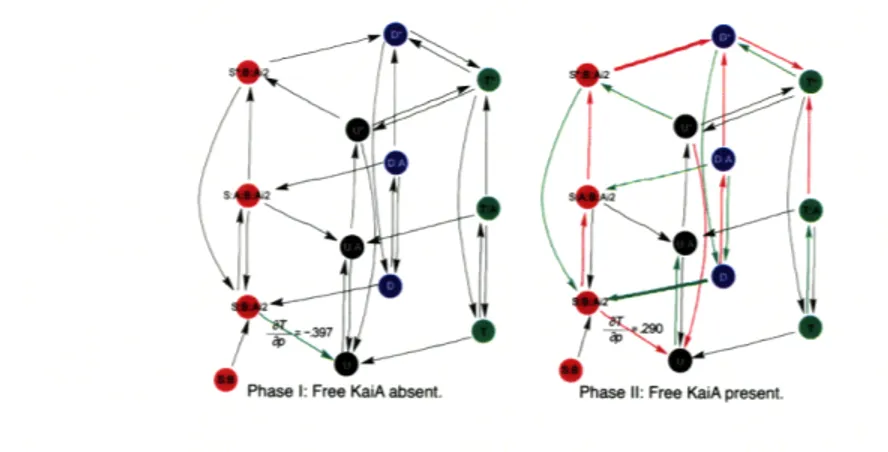
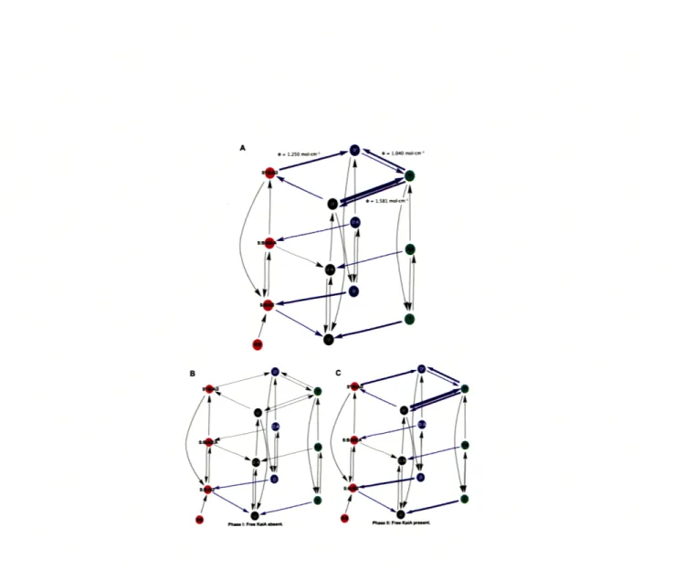
Figure 5-2 shows an abstracted visual representation and illustrates relative reac-tion rates (Figure A-1(I) in SI for the full model). The arrow thicknesses represent reaction rates, which are weighted logarithmically according to magnitude, with the thickest arrows representing the fastest kinetics. The reaction rates along the planes for phosphoform interconversion are equivalent in the mass action model and the Rust et al. model (Figure A-1(II) in SI). Allosteric regulation of KaiC by free KaiA runs perpendicular to these planes, and the combinatorial intermediate binding states in the assembly and disassembly kinetics of the KaiABC complex are noticeably col-lapsed in this abstraction (Figure A-1(III) and A-1(IV) in SI).

Figure 5-2: Abstracted Visual Representation of the Mass Action Model. Here is an abstraction of our mass action model where arrow thicknesses represent reaction rates that are weighted logarithmically according to magnitude where the thickest arrows represent the fastest kinetics. The reaction rates are approximately:

> 1 (thick arrow), > 0.1 (medium arrow), < 0.1 (thin arrow).

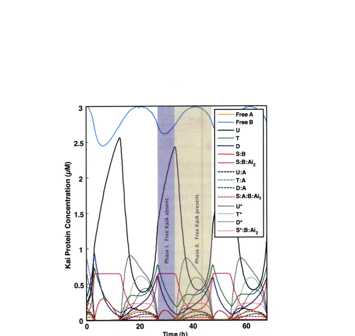
The time course of these appreciable KaiC complexes, free KaiA, and free KaiB are plotted in Figure 5-3. We identify two regimes (Phase I and Phase II) of Kai protein behavior within the circadian period. Phase I is characterized by the absence of free KaiA, progressive dephosphorylation of KaiC species, and saturation of the S-KaiC:KaiB with sequestered KaiA. Phase II is characterized by the appearance of activated KaiC species (D*,S*,T*,U*), the presence of free KaiA, and a prepon-derance of phosphorylation kinetics. During dephosphorylation, essentially only the lower plane of Figure 5-2 is populated because free KaiA is necessary to activate KaiC species to the middle (Michaelis complex) and upper planes. In the lower plane, un-activated KaiC species can only dephosphorylate. Phase II populates the entire figure and drives the oscillatory dynamics in a manner that can be tracked but isn't readily understood. Further analysis of the model is necessary to reveal relationships between network structure and oscillatory dynamics.

Figure 5-4 shows the sensitivities of the oscillatory period with respect to the rel-ative rate parameters of the model. The arrow thicknesses represent scaled period sensitivities that are weighted logarithmically according to the highest magnitude,

2.5 - D S:B - S:B:Ai2 --- U:A 2 --- T:A .--- D:A --- S:A:B:Ai2 o ... D* ... _S*:B:Ai 2 0 1.5 0 20 40 60 Time (hi

Figure 5-3: Time Course Trajectories of Species Concentrations. Here we plot the trajectories of the species (state variables) that occur at appreciable con-centrations. The presence or absence of free KaiA in the model drives two regimes of behavior, Phase I and Phase II, within the circadian period. During autokinase (Phase II), unactivated S-KaiC binds to KaiB and sequesters free KaiA to form the KaiABC complex, as shown by the magenta trajectory. Furthermore, all free KaiA in the system is sequestered during autophosphatase (Phase I).

0 W

Figure 5-4: Scaled Period Sensitivities .logT Period sensitivities are imposed on this abstracted visual representation of the mass action model. The arrow thicknesses represent period sensitivities that are weighted logarithmically according to the high-est magnitude where red is positive sensitivity and green is negative sensitivity. The period sensitivity magnitudes are approximately: > 1 (thick arrow), > 0.1 (medium arrow), < 0.1 (thin black arrow).

with red being positive sensitivity, green being negative and black being close to zero. The positive (red) sensitivity on the reaction rate kd has a dominant length-ening effect on the period that may be compensated by the shortlength-ening effect due to kI. 5 These phosphorylation and dephosphorylation dynamics between S-KaiC and

D-KaiC play a significant role in modulating the period. The allosteric regulation of free KaiA supports the self-consistent processes that phosphorylated KaiC (excluding T-KaiC) activation slows the circadian period and phosphorylated KaiC inactivation speeds the circadian period. The reverse behavior occurs for unphosphorylated KaiC as shown in Figure 5-4.

To understand better the system behavior between the two phases, we partitioned the circadian period into a dephosphorylation interval (Phase I) and a phosphorylation interval (Phase II) as shown in Figure 5-5. According to our initial observations from Figure 5-3, we tracked species concentrations separately during these two regimes. To track species concentrations in a given interval, partitioning of the species was accomplished by enzyme-driven switch-like behavior. During the dephosphorylation

A - D-KaiC so - S-KaiC so T-KaiC U-KaiC 20 260 0 20 40 60 80 C 200- _{0 A} .40W4 20 'RO 0 0 0Y 0 20 40 60 80 0 20 40 60 80 Time (h)

Figure 5-5: Circadian Period Decomposition. The mass action model was de-composed into a dephosphorylation interval (B) and a phosphorylation interval (C) by implementing enzyme-driven switch-like behavior (D). (A) The superimposition of Phases I (B) and II (C) results in the full trajectories of the mass action model.

interval, the switch was in 'off' mode due to the absence of free KaiA; likewise during the phosphorylation interval, the switch was in the 'on' mode due to the presence of free KaiA.

In order to track KaiC autokinase and autophosphatase, we created an artificial species which was activated by KaiA and would bind and track KaiC behavior. Since free KaiA exists at a much lower concentration than the amount of artificial species required to complex with KaiC (KaiATotal < KaiCTotal), an enzyme cascade was im-plemented as a rapid two-step process: (1) continual activation of a low concentration enzyme XE, where XE < KaiATotal, which then (2) activated a high concentration species X* , where X*> KaiCTotal, to rapidly and repeatedly complex with all KaiC phosphoforms. This enzyme cascade persisted exclusively during the 'on' mode; con-sequently X* would remain uncomplexed to KaiC once free KaiA depleted and the dephosphorylation interval initiated. As a result, all KaiC complexes in Phase II were

0 20 40 60 80 D XE ~~~~ ~uwi

rrn

Phase II: Free KaiA present.

Figure 5-6: Scaled Period Sensitivities ioT for the Decomposed Period. The dephosphorylation (left) and phosphorylation (right) intervals of a circadian period is shown here. The transition from unactivated S-KaiC to unactivated U-KaiC plays the most significant role in setting the period during KaiC dephosphorylation. Conversely, an array of kinetics influence the periodicity during KaiC phosphorylation. The arrow thicknesses and colors represent period sensitivities that are weighted logarithmically according to the same spread for period sensitivities in Figure 5-4.

bound to X* and thus differentiable in a computational experiment sense from KaiC complexes in Phase I, which were not bound to this enzyme. Through the imple-mentation of this enzyme cascade, we were able to track transients of the system (for implementation see Tables A.12 and A.13 in SI).

Perturbation analysis of the in vitro circadian oscillator for S. elongatus has shown that modulations of KaiC autokinase and autophosphatase kinetics have had the most dramatic effects on period setting [29]. By performing period sensitivity analysis on each dephosphorylation interval (Phase I) and phosphorylation interval (Phase II) we were able to decompose the influence that free KaiA allosteric regulation has on KaiC phosphoform interconversion. The transition of unactivated S-KaiC to U-KaiC was determined to be a triggering process during dephosphorylation for setting the period. As shown in Figure 5-6 (left), this autophosphatase process has an overall shortening effect on the period, being the singular influence particularly when free KaiA is absent from the system. Although this same transition has the reverse effect on the period in the presence of KaiA, there are also other kinetics at play according to the heavily weighted sensitivities in the diagram. Upon closer inspection of Figure

5-6 (right), the decomposed period sensitivities during the phosphorylation interval (Phase II) are comparable in magnitude and effect to the computed full period sen-sitivities in Figure 5-4.

Analyzing the flux pathways for a circadian period provides further insight into domi-nant processes within the model. As shown in Figures 5-7A and 5-7C, the notion that the flux during the phosphorylation interval is comparable to the overall period flux is in agreement with our full period sensitivity results, indicating that the processes in the presence of free KaiA are dominant in setting a faster or slower circadian clock. A more intuitive interpretation of this figure is that activity during the dephospho-rylation interval occurs mainly on KaiC in the unactivated state (Figure 5-7B), due to the fact that all activated KaiC has autodephosphorylated due to the absence of free KaiA in the system.

Yet counterintuitive to our earlier results is that a majority of the system flux distri-bution is through a process with relatively negligible period sensitivity (Figure 5-4), from activated U-KaiC to T-KaiC; this flux then splits to where half cycles back to activated U-KaiC and the remainder becomes phosphorylated at the serine site 5-7A. According to Rust et al. observations the sequence of phosphoform interconversion goes along the activated U-KaiC to T-KaiC, then activated T-KaiC to D-KaiC path-way. On the contrary, our flux analysis determines that near equivalent amounts of activated T-KaiC and S-KaiC are converted into the doubly phosphorylated form 5-7A. Other phosphoform interconversions leading to significant fluxes are along the processes with higher period sensitivities, although not all are accounted for.

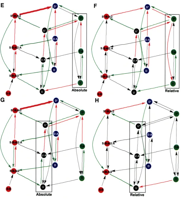
Supplemental analysis on the scaled peak-to-peak phase sensitivities, and scaled ab-solute and relative amplitude sensitivities for the full period is uniform in denot-ing processes of interest. When compardenot-ing sequential peaks of KaiC phosphoforms, particularly the T-KaiC to D-KaiC phase sensitivities appear to have a significant influence on the ordered phosphorylation timing circuitry. In Figure 5-8B for the

T-P P: , WIM1Fl-w

Figure 5-7: Flux Pathways for the Phosphoform Interconversion during the Full and Decomposed Period. The phosphoform flux distribution is shown here for a full period along with the flux distribution for the desphosphorylation interval (bottom, left) and phosphorylation interval (bottom, right) for the same period. The majority of the flux distribution occurs during the phosphorylation interval, specif-ically from activated U-KaiC to activated T-KaiC. The arrow thicknesses represent the overall flux for each time course according to the highest magnitude, where the

magnitudes are approximately: > 4 (thick blue arrow), 4 > D > 1 (medium blue arrow), > 0.1 (thin blue arrow), < 0.1 (thin black arrow). Not graphed here are the fluxes orthogonal to the phosphoform interconversion planes, on account of these reaction rates being invariably parameterized on a faster time-scale.