HAL Id: hal-03175811
https://hal.archives-ouvertes.fr/hal-03175811
Preprint submitted on 21 Mar 2021
HAL is a multi-disciplinary open access archive for the deposit and dissemination of sci-entific research documents, whether they are pub-lished or not. The documents may come from teaching and research institutions in France or abroad, or from public or private research centers.
L’archive ouverte pluridisciplinaire HAL, est destinée au dépôt et à la diffusion de documents scientifiques de niveau recherche, publiés ou non, émanant des établissements d’enseignement et de recherche français ou étrangers, des laboratoires publics ou privés.
Distributed under a Creative Commons Attribution| 4.0 International License
A Neural Network for Semigroups
Edouard Balzin, Boris Shminke
To cite this version:
EDOUARD BALZIN, BORIS SHMINKE
Abstract. Tasks like image reconstruction in computer vision, matrix completion in recommender systems and link prediction in graph theory, are well studied in machine learning literature. In this work, we apply a denoising autoencoder-based neural network architecture to the task of completing partial multiplication (Cay-ley) tables of finite semigroups. We suggest a novel loss function for that task based on the algebraic nature of the semigroup data. We also provide a software package for conducting experiments similar to those carried out in this work. Our experiments showed that with only about 10% of the available data, it is possible to build a model capable of reconstructing a full Cayley from only half of it in about 80% of cases.
Contents
1. Introduction 1
2. Basics of semigroups 4
3. Experimental setup 6
4. Results and discussion 10
References 12
1. Introduction
Semigroups. A semigroup structure is one of the basic algebraic struc-tures that one can put on a set S. It consists of a binary operation S × S → S, (x, y) 7→ x · y that satisfies the associativity identity: that is, for all x, y, z in S, one requires x · (y · z) = (x · y) · z. The exam-ples of such structures are many: groups and monoids, for example, come equipped with associative binary operations. For another exam-ple, given a (small) category C, denote Mor C the set of all morphisms, take S = MorC∪{0} and put f ·g = f ◦g if the composition is well de-fined and 0 otherwise. IfC has more than one object, the result will be
Table 1. Number of equivalence classes of semigroups up to isomorphism or anti-isomorphism [1].
Cardinality # semigroups up to equivalence
1 1 2 4 3 18 4 126 5 1,160 6 15,973 7 836,021 8 1,843,120,128 9 52,989,400,714,478
a semigroup that does not come from a monoid. Semigroup examples also appear from automata.
If we restrict our attention to finite semigroups, the existing classi-fication tables [1] are very counter-intuitive to any mathematician fa-miliar with finite groups. Semigroups, classified up to an isomorphism or anti-isomorphism (Definition 2.3), exist in abundance, as per Table 1 (to compare, there is only one finite group structure on a set of seven elements). While certain results of classification exist, the most known one being the Krohn–Rhodes decomposition theory [5], understanding semigroups of cardinality (or order) up to 20 remains a challenging task.
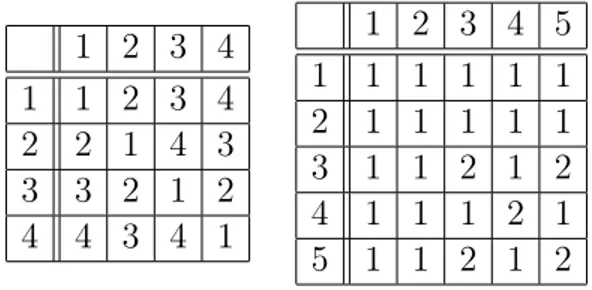
1.1. Machine learning of semigroups. This paper is our first at-tempt to see if one can approach questions about semigroups using the methods of machine learning. As a first question, we wanted to see how we could explain what a semigroup is to a neural network, so that the latter captures the algebraic character of the semigroup structure. Given a finite set S, we can order its elements and present any binary operation m : S × S → S as a multiplication table. A couple of examples is given in Table 2. Such tables can be transformed into a neural network input if viewed as tensors in (Rn)3, where n is the cardinality of S. Such a tensor denoted (Mijk) takes values Mijk = 1 if the i’th element times the j’th element equals the k’th element, and Mijk = 0 in all other cases.
Table 2. Multiplication tables of Klein 4-group Z/2Z × Z/2Z and of a 3-nilpotent semigroup on 5 elements.
1 2 3 4 1 1 2 3 4 2 2 1 4 3 3 3 2 1 2 4 4 3 4 1 1 2 3 4 5 1 1 1 1 1 1 2 1 1 1 1 1 3 1 1 2 1 2 4 1 1 1 2 1 5 1 1 2 1 2
The lack of classification of semigroups of higher order led us to imagine, then, the following question: can one start with a multiplica-tion table that is partially filled, and ask a neural network provide a completion? This can be formulated as an autoencoder [2] problem on (Rn)3.
In this paper, we have chosen n = 5. As noted above, semigroups of cardinality 5 are already classified, and while our goal would be to move into higher cardinalities, it is still of use to study a known list of semigroups to propose a kind of neural network that is useful for under-standing semigroup structure. Unlike in the problem of solving sudoku [4] (also a problem of table completion that inspired some reflection behind this project), we cannot rely on image-processing techniques and related convolutional neural networks as they do not adequately measure the structure of semigroups. The analysis of n = 5 case helped us to formulate the problem and design the architecture that worked.
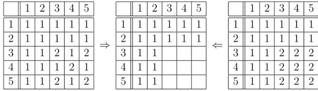
The 1160 equivalence classes of n = 5 correspond (as can be seen from [1, 9]) to 183732 different tables, which is provides a sufficient amount of data for our purposes. For the input of the autoencoder in this case, both for training and testing, we take a table that is produced from a semigroup by forgetting some multiplications, which corresponds to “erasing” certain cells in the multiplication table. The output tensor, the value of the autoencoder on such a partially filled table, would have to correspond to a) a table that b) is associative. In the context of supervised learning, the condition b) can be enforced with different choices of loss functions. One choice would simply pe-nalise the difference between the reconstructed table and the original one. This choice is unnatural mathematically as tables can have non-unique completions (Table 3) and also relies on knowing the resulting semigroup.
Table 3. Different semigroups giving the same partially filled table. 1 2 3 4 5 1 1 1 1 1 1 2 1 1 1 1 1 3 1 1 2 1 2 4 1 1 1 2 1 5 1 1 2 1 2 ⇒ 1 2 3 4 5 1 1 1 1 1 1 2 1 1 1 1 1 3 1 1 4 1 1 5 1 1 ⇐ 1 2 3 4 5 1 1 1 1 1 1 2 1 1 1 1 1 3 1 1 2 2 2 4 1 1 2 2 2 5 1 1 2 2 2
Another, called the associator loss (3.1 below), translates the asso-ciativity of semigroup multiplication into a certain probabilistic func-tion on the neural network. This choice accepts associative answers different from the original table and, interestingly, does not require one to actually present a semigroup that completes the partially filled table.
1.2. Acknowledgements. The authors of this paper are very grateful to Jordan Emme, Wesley Fussner and Carlos Simpson for their remarks. This work has been supported by the French government, through the 3IA Côte d’Azur Investments in the Future project managed by the National Research Agency (ANR) with the reference number ANR-19-P3IA-0002.
2. Basics of semigroups
Definition 2.1. A semigroup is a set S together with a binary opera-tion · : S × S → S, (a, b) 7→ a · b, that is associative: for all a, b, c in S, one has a · (b · c) = (a · b) · c.
One could thus say that a semigroup is an associative magma, or a non-unital monoid. Various monoids and groups provide examples of semigroups if we forget the extra properties (existence of units, in-verses). In this paper, we only consider the case when the set S is finite. We shall write (S, ·) to denote a semigroup or simply S when this does not lead to confusion.
Notation 2.2. Let (S, ·) be a semigroup. Its opposite semigroup will be denoted Sop = (S, ·op). Its underlying set is S and the multiplication operation ·op is defined as a ·op b := b · a.
Definition 2.3. A homomorphism, or simply a morphism of semi-groups (S, ·) → (T, ∗) is a map of sets f : S → T such that for all a, b ∈ S, one has f (a) ∗ f (b) = f (a · b). Two semigroups S, T are called equivalent if there is an isomorphism between S and T or between S and Top (the latter meaning that S and T are anti-isomorphic).
A semigroup map f is an isomorphism if and only if it is a bijection of the underlying sets.
Just like with finite groups, the multiplication of finite semigroups can be described in terms of a multiplication table. Our work deals with those tables viewed as certain tensors that can be obtained as follows.
Definition 2.4. Let (S, ·) be a semigroup and k a field (one can assume k = R for the purposes of machine learning). Its associated semigroup algebra k[S] is a non-unital k-algebra defined as follows. As a vector space, k[S] =∼= k|S| is the free vector space on S, and the multiplication operation is extended from · by k-bilinearity: (P
iλiai)( P
jµjbj) := P
i,jλiµj(ai· bj).
Any semigroup morphism S → T induces a non-unital algebra mor-phism k[S] → k[T ], and one has k[Sop] = k[S]op.
The multiplication operation, being bilinear, can be viewed as a map m : k[S] ⊗ k[S] → k[S]. When S is finite, the semigroup algebra k[S] is finite-dimensional as a vector space, and so we can view the multiplication as a tensor m ∈ (k[S]∗)⊗2⊗ k[S].
From now on, assume that S is finite of cardinality n. If one denotes S = {ei}ni=1, then the eiand their dual linear forms fjform bases of k[S] and k[S]∗, respectively. The multiplication m can then be expressed as
m = n X i,j,k=1
Mijkek⊗ fi⊗ fj,
where Mijk is equal to 1 if ei· ej = ek and is 0 otherwise.
Definition 2.5. For a finite semigroup S, the coefficients (Mijk) are called the structure constants of S. In this work, we shall also refer to (Mijk) as the Cayley table of S.
Remark 2.6. If instead of k[S] we considered a general non-unital k-algebra A that is finite dimensional as a k-vector space, with a basis that one can also denote ei, the coefficients Mijkobtainable in the same way from the multiplication A ⊗ A → A would not consist only of 0’s
and 1’s. The associativity condition for the basis vectors, (ei· ej) · ek= ei· (ej · ek) gives the following equation on the coefficients:
(2.1 ) X
m
(MijmMmkl− MimlMjkm) = 0.
A typical presentation of Mijk is usually done in a table format, by putting ek or simply its index k in the ij-cell (as done in Table 2 above). One can imagine such a multiplication table being partially filled, with some multiplications ei · ej not specified, an idea that we formalise below.
3. Experimental setup
3.1. Data representation. Given a set S = {ei}ni=1, consider a func-tion F : S × S × S → [0, 1]. We would like to treat this funcfunc-tion as a probability distribution for the potential multiplication: P(ei · ej = ek) = F (ei, ej, ek). For this to make sense, the function F must satisfy the following condition: P
kF (ei, ej, ek) = 1 for all possible choices of i and j.
Definition 3.1. Call such a function F a partial Cayley table. A partial Cayley table F is filled at 1 ≤ i, j ≤ n if there exists k such that F (i, j, k) := F (ei, ej, ek) = 1.
Any semigroup structure on S provides us with the partial Cayley table F (i, j, k) = Mijk that is actually filled at all i, j. Our definition does not guarantee however that a partial Cayley table that is filled at all i, j corresponds to an associative multiplication. For this reason, define:
Definition 3.2. A partial Cayley table F : S ×S ×S → [0, 1] is solvable if there exists a semigroup structure on S, with structure constants (Mijk), such that Mijk = F (i, j, k) for all i, j at which F is filled.
As noted in the introduction, a solvable F can have multiple semi-group solutions.
We can store F (i, j, k) as a tensor of one axis of dimension n3 (in [6] parlance), e.g. using a lexicographical order of triples of indices (i, j, k). These tensors are used as the main method of data representation in this work.
Assume now that for a set S we specified only some multiplications for a semigroup structure. This allows us to partially define the func-tion F . If the result of multiplicafunc-tion ei · ej is not specified, we can
Figure 1. Translating a multiplication table into as a partially filled F : {0, 1, 2, 3}3 → [0, 1].
extend by employing a uniform distribution in such cases, i.e. assume in that case that F (i, j, k) = n1 for all k (Figure 1).
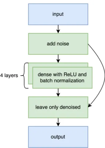
3.2. Network architecture. One can consider a partial Cayley table as a result of distortion of a corresponding fully filled table. Similarly, arbitrary probabilistic tensors can be viewed as noisy counterparts of zero-or-one tensors. A well-known way to get rid of distortions and restore the original of an image is by using a denoising autoencoder [2]. For a scheme of the autoencoder architecture used in this paper see Figure 2. Besides adding noise to its input, this network also cleans its output of guesses of the cells which were not masked during noise addition; these cells correspond to known fillings of the Cayley table. In other words, if the input was filled at i, j so that ei· ej = el and the output F (i, j, k) during the forward pass is a float between 0 and 1, it then redefined as F (i, j, k) := 0 or 1 corresponding to k 6= l or k = l.
Another particular thing to note is that usually we have encoders which move from higher dimensions to lower ones. Here we have input and output both of dimension n3and the hidden layers all of dimension n5.
For more details we invite the reader to consult the source code available at [9].
3.3. Loss functions. If x is an input for an autoencoder and y is its output, we can define its loss function L (x, y) in a variety of ways.
Figure 2. Autoencoder architecture used to generate Cayley tables. The arrow from the input with added noise to the “leave only denoised” layer corresponds to restoring the values of initially known cells.
Since in our case values of x and y are probabilities of a joint distri-butions, it could be a good idea to use some measure of dissimilarity between these two distributions, e.g. their Kullback-Leibler divergence:
KL (x, y) := n X i=1 xilog xi yi .
Note that this choice of a loss function does not explicitly enforce any notion of associativity. The problem with this function is that after applying corruption to x it can often be recovered as y non-uniquely, yet the loss function (x, y) 7→ KL(x, y) will prefer y = x to any other value of y, even if that value is associative.
Another choice of a loss function is what we call the associator loss. First, remember that y corresponds to the probability distribution yijk = P {ei· ej = ek}. Then we can calculate probabilities of double multiplications: P {(ei· ej) · ek= el} = n X m=1 P {em· ek= el|ei· ej = em} P {ei· ej = em} = n X m=1 ymklyijm.
Now we can define the loss function as a KL-divergence between the distributions P {(ei · ej) · ek = el} and P {ei· (ej · ek) = el}:
(3.1 ) AL (x, y) := KL n X m=1 yijmymkl, n X m=1 yimlyjkm ! .
This loss does not depend on x but only on probabilistic associativity of y, and indeed it corresponds to interpreting in probabilistic terms the coefficient equation (2.1 ) of Remark 2.6.
3.4. Noise. In our case, the noise which autoencoder is treating cor-responds to the absence of some number of cells in a Cayley table. In our experiments, both for training and testing, we take tables of semi-groups of cardinality 5. Given any table F : S × S × S → R we then add noise by re-setting F (i, j, k) = 15 for i, j corresponding to randomly chosen 50% of cells of the original Cayley table.
3.5. Training and testing datasets. For this work we use an exten-sive database of finite semigroups up to eight elements from [1]. If we fix the number of elements that is less or equal to 8, we get the number of classes of equivalence of semigroups (Definition 2.3) as well as their presentation in [1]. In this paper, we used semigroups of 5 elements for experiments: as mentioned, this corresponds to 1160 classes and 183732 potential tables.
In detail, we proceeded by dividing this set of 1160 equivalence classes into three subsets: training, validation, and testing in propor-tion 10/10/80. We then produced all Cayley tables of isomorphic and anti-isomorphic semigroups corresponding to these classes of equiva-lence, a procedure that one can view as a form of data augmentation. Finally, we applied the noise as described in the previous section, but
only to validation and testing sets. The training set gets its noise dur-ing the traindur-ing process, and 50% of cells to be masked are chosen at random for every batch, and are not fixed in advance for all the training process. Note that all partial tables appearing here are solvable. 3.6. Quality metrics. Since we train autoencoders, it is natural to use the following metrics:
Definition 3.3. The guess rate is the percentage of outputs of a net-work which coincide with their inputs before applying noise. The as-sociative rate is the percentage of outputs of a network which satisfy the assoiciativity condition.
The associative rate appears to be a better quality metric, since we are interested not in exact reconstruction of inputs but in generating associative tables. A half-filled table can be completed to different semigroups, but the guess rate will only accept the original table for its score.
3.7. Training process. We trained all the networks using the Pytorch [6] framework, using an Adam optimizer [3] with the learning rate set to 0.0001. The training was done for a maximum of 1000 epochs with an early stopping applied if the loss did not go down for ten consecutive epochs. The training was done on [7] cloud resources and took several hours in total. We performed batch normalisation on each layer and used random network parameter initialisation.
4. Results and discussion
First, we note that teaching an autoencoder to simply reconstruct its input without knowing anything about associativity proved to be not only unnatural but in fact bringing poorer results. Even in terms of its main goal – finding the original table from the input with added noise – the KL divergence loss is less adequate than the associator loss (AL): see Table 4 for exact numbers. One way to interpret the KL-AL guess ratio difference might be in observing that the AL network does better at the associativity task overall, in particular it does better at reconstructing the original table.
The AL network results are rather promising. We managed to pro-duce a full associative table given only a half of filled cells as an input in 82% of cases. That is even more impressive given that we relied only on 10% of all available tables from the database, thus managing
Table 4. Comparison of impacts of a loss function choice. The associator loss network fares better not only at producing associative tables, but also at guessing the original table to which we applied noise.
Loss function used Guess rate Associative rate KL divergence 0.0977 0.5838 Probabilistic associator loss 0.1453 0.8212
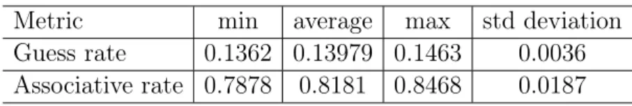
Table 5. Comparison of impacts of training set choice on guess and associative rates (AL network).
Metric min average max std deviation Guess rate 0.1362 0.13979 0.1463 0.0036 Associative rate 0.7878 0.8181 0.8468 0.0187
to generalise to 80% (which went to the test set). Our results remain dependant on the choice of these 10% tables for a training set, with deviation representing about 2 percent of the loss (see Table 5 for the details).
These findings make us believe that an AL-type network could also be successfully used for higher cardinalities. One could view the as-sociator loss as the suitable "architectural adaptation" to the case of semigroups: instead of convolutional layers, we are dealing with alge-braic equations written into the loss function, in probabilistic terms. Such a neural network can work on higher-dimensional data if adapted properly. In fact, it can even accept as training set partial tables that are known to be solvable; the latter can be verified with various model searchers such as Mace4/Prover9 [8].
And if one is able to produce a train dataset in higher cardinalities, the trained network can be viewed as a certain generator, that produces full tables out of sets of identities corresponding to known cells in the input. We do not know if all possible tables can be produced in such a way, and verifying it for lower cardinalities is one of our future goals. For the higher cardinality, one could ask if such a neural network could produce any semigroup in its image if fed with random input. Finally, one can imagine generalisations of such neural networks to other classes of algebraic structures.
References
[1] Andreas Distler, James Mitchell, GAP Package Smallsemi, https://www. gap-system.org/Packages/smallsemi.html
[2] Ian Goodfellow, Yoshua Bengio and Aaron Courville, Deep Learning Book, Mit Press 2016, https://www.deeplearningbook.org
[3] Diederik P. Kingma, Jimmy Ba, Adam: A Method for Stochastic Optimization, 3rd International Conference for Learning Representations, San Diego, 2015, https://arxiv.org/abs/1412.6980
[4] Kyubyong Park, Can Convolutional Neural Networks Crack Sudoku Puzzles? https://github.com/Kyubyong/sudoku
[5] Jean-Éric Pin, Mathematical Foundations of Automata Theory, https://www. irif.fr/~jep/PDF/MPRI/MPRI.pdf
[6] PyTorch Website https://pytorch.org/
[7] Google Colaboratory Website https://colab.research.google.com/ [8] Prover9 and Mace4, https://www.cs.unm.edu/~mccune/prover9/
[9] Neural Semigroups version 0.3.8, GitHub https://github.com/inpefess/ neural-semigroups/tree/v0.3.8
![Table 1. Number of equivalence classes of semigroups up to isomorphism or anti-isomorphism [1].](https://thumb-eu.123doks.com/thumbv2/123doknet/12968781.377494/3.918.272.642.226.460/table-number-equivalence-classes-semigroups-isomorphism-anti-isomorphism.webp)
![Figure 1. Translating a multiplication table into as a partially filled F : {0, 1, 2, 3} 3 → [0, 1].](https://thumb-eu.123doks.com/thumbv2/123doknet/12968781.377494/8.918.248.718.148.426/figure-translating-multiplication-table-partially-filled-f.webp)