Economic Growth Evens-Out Happiness: Evidence from Six Surveys

(1)

HAL Id: hal-01080877

https://hal-pjse.archives-ouvertes.fr/hal-01080877

Preprint submitted on 6 Nov 2014

HAL is a multi-disciplinary open access archive for the deposit and dissemination of sci-entific research documents, whether they are pub-lished or not. The documents may come from teaching and research institutions in France or abroad, or from public or private research centers.

L’archive ouverte pluridisciplinaire HAL, est destinée au dépôt et à la diffusion de documents scientifiques de niveau recherche, publiés ou non, émanant des établissements d’enseignement et de recherche français ou étrangers, des laboratoires publics ou privés.

Economic Growth Evens-Out Happiness: Evidence from

Six Surveys

Andrew E. Clark, Sarah Flèche, Claudia Senik

To cite this version:

Andrew E. Clark, Sarah Flèche, Claudia Senik. Economic Growth Evens-Out Happiness: Evidence from Six Surveys. 2014. �hal-01080877�

(2)

WORKING PAPER N° 2014

– 37

Economic Growth Evens-Out Happiness:

Evidence from Six Surveys

Andrew E. Clark Sarah Flèche Claudia Senik

JEL Codes: D31, D6, I3, O15

Keywords: Happiness, inequality, economic growth, development, Easterlin paradox

P

ARIS

-

JOURDAN

S

CIENCES

E

CONOMIQUES

48, BD JOURDAN – E.N.S. – 75014 PARIS TÉL. : 33(0) 1 43 13 63 00 – FAX : 33 (0) 1 43 13 63 10

www.pse.ens.fr

CENTRE NATIONAL DE LA RECHERCHE SCIENTIFIQUE – ECOLE DES HAUTES ETUDES EN SCIENCES SOCIALES

(3)

1

Economic Growth Evens-Out Happiness: Evidence from Six Surveys*

Andrew E. Clark† (Paris School of Economics - CNRS) Sarah Flèche§ (CEP, London School of Economics)

Claudia Senik‡ (University Paris-Sorbonne and Paris School of Economics)

October 2014

Abstract

In spite of the great U-turn that saw income inequality rise in Western countries in the 1980s, happiness inequality has fallen in countries that have experienced income growth (but not in those that did not). Modern growth has reduced the share of both the “very unhappy” and the “perfectly happy”. Lower happiness inequality is found both between and within countries, and between and within individuals. Our cross-country regression results argue that the extension of various public goods helps to explain this greater happiness homogeneity. This new stylised fact arguably comes as a bonus to the Easterlin paradox, offering a somewhat brighter perspective for developing countries.

Keywords: Happiness, inequality, economic growth, development, Easterlin paradox. JEL codes: D31, D6, I3, O15.

* We are very grateful to two anonymous referees for pertinent and helpful suggestions. We thank seminar participants at Ca’Foscari University (Venice), the Conference on “Happiness and Economic Growth” (Paris), the Fifth ECINEQ conference (Bari), the Franco-Swedish Program in Philosophy and Economics Well-being and Preferences Workshop (Paris), ISQOLS12 (Berlin), LSE, Namur, the OECD workshop on Subjective Wellbeing (Paris), the 2013 Royal Economic Society Conference (London) and Universitat Autònoma de Barcelona. Many people have given us good advice: we thank Dan Benjamin, François Bourguignon, Daniel Cohen, Jan-Emmanuel De

(4)

2 Neve, Richard Easterlin, Yarine Fawaz, Francisco Ferreira, Ada Ferrer-i-Carbonell, Paul Frijters, Sergei Guriev, Ori Heffetz, Tim Kasser, John Knight, Richard Layard, Sandra McNally, Andrew Oswald, Nick Powdthavee, Bernard van Praag, Eugenio Proto, Martin Ravallion, Paul Seabright, Conal Smith and Mark Wooden. The BHPS data were made available through the ESRC Data Archive. The data were originally collected by the ESRC Research Centre on Micro-social Change at the University of Essex. The German data used in this paper were made available by the German Socio-Economic Panel Study (SOEP) at the German Institute for Economic Research (DIW), Berlin. The Household, Income and Labour Dynamics in Australia (HILDA) Survey was initiated and is funded by the Australian Government Department of Families, Housing, Community Services and Indigenous Affairs (FaHCSIA), and is managed by the Melbourne Institute of Applied Economic and Social Research (Melbourne Institute). Neither the original collectors of the data nor the Archives bear any responsibility for the analyses or interpretations presented here. We thank CEPREMAP and the French National Research Agency, through the program Investissements d'Avenir, ANR-10-LABX_93-01, for financial support; this work was also supported by the US National Institute on Aging (Grant R01AG040640) and the Economic & Social Research Council. † PSE, 48 Boulevard Jourdan, 75014 Paris, France. Tel.: +33-1-43-13-63-29. E-mail:

Andrew.Clark@ens.fr.

‡ Centre for Economic Performance, London School of Economics and Political Science, Houghton Street, London WC2A 2AE, UK. E-mail: S.Fleche@lse.ac.uk.

§ PSE, 48 Boulevard Jourdan, 75014 Paris, France. Tel.: +33-1-43-13-63-12. E-mail: senik@pse.ens.fr.

(5)

3

I. Introduction

“Will raising the incomes of all increase the happiness of all?” Richard Easterlin asked somewhat ironically in 1995 (Easterlin, 1995), having shown that average self-declared happiness generally does not increase over the long run, even during episodes of sustained economic growth (Easterlin, 1974). This finding has helped inspire a vast empirical and theoretical literature on social comparisons and adaptation (as surveyed in Clark et al., 2008). Easterlin’s original finding has more recently been called into question, with it being suggested that in some countries there is a positive time-series correlation between per capita GDP and average levels of subjective well-being (a well-known contribution to this extent is Stevenson and Wolfers, 2008a). At the same time as this ongoing debate about the relationship between the average happiness level and GDP growth, a striking new stylised fact has recently emerged regarding the distribution of happiness or “happiness inequality”. As documented in Clark et al. (2014), there is strong evidence across a wide variety of datasets that GDP growth is associated with systematically lower levels of happiness inequality (where this latter is picked up by the coefficient of variation). It is this happiness-inequality literature to which we wish to contribute here.

We provide evidence that economic growth is systematically correlated with a more even distribution of subjective well-being. This correlation for the most part holds despite the associated rise in income inequality, does not seem to be the result of any statistical artefact, is found in almost all domains of satisfaction, but is not found in placebo tests on other subjective variables. We suggest the extension of the provision of public goods as one likely candidate explanation for the lowering of happiness inequality.

None of our analyses of countries over time reveal a significant relationship between GDP growth and average happiness. It is this finding that has attracted great attention, as it suggests that

(6)

4 economic growth may serve no (happiness) purpose. Outside of a utilitarian world, however, we may be more Rawlsian and give a certain weight to the avoidance of misery: here higher GDP does seem to chalk up points. The value we attach to GDP growth will then depend on the particular social-welfare function that we have in mind.

The remainder of the paper is organised as follows. Section 2 shows that higher income is associated with a tighter distribution of subjective well-being across countries, within countries, across individuals, and within individuals. Section 3 then presents a regression analysis emphasising the key roles of income inequality and public goods in determining happiness inequality. Section 4 considers a number of additional tests regarding the measurement of dispersion, the issue of time in panel (for our panel data results), and some placebo tests. Last, Section 5 concludes.

2. Income Growth and Happiness Inequality

There is a great deal of work using country-level data attempting to show a relationship, or the lack of one, between GDP growth and average levels of satisfaction or happiness over time. However, until very recently, little attention was paid to inequality in subjective well-being as economies grew. Knowing that average happiness scores remained broadly unchanged does not tell us anything about the distribution of well-being: flat happiness time profiles can be associated with a stable distribution of happiness, rising inequality, or lower inequality.

Two papers, Stevenson and Wolfers (2008b) and Dutta and Foster (2013), have explicitly addressed this issue. Both papers consider American General Social Survey (GSS) data from the early 1970s onwards (although their analytical approach differs); both underline a general fall in the inequality of happiness in the US up to around 2000, followed by an inversion of the trend (i.e. rising

(7)

5 happiness inequality). Veenhoven (2005) found falling happiness inequality in EU countries (surveyed in the EuroBarometer) over the years 1973-2001, in spite of rising income inequality. He also notes a tighter distribution of happiness in “modern nations” rather than more traditional countries.

Clark et al. (2014) then looked at this issue systematically, using a wide variety of different datasets and a long time period (1970-2010). The crux of their argument is that countries with growing GDP per capita have also experienced falling happiness inequality. The data used there come from the World Values Survey (WVS), the German socio-economic panel (SOEP), the British Household Panel Survey (BHPS), the American GSS and the Household, Income and Labour Dynamics in Australia survey (HILDA). Happiness inequality was picked up by the coefficient of variation (the standard deviation of happiness divided by the sample happiness mean).

It is difficult to know what the correct measure of the distribution of subjective well-being is. One worry is that higher happiness levels will mechanically lead to lower dispersion as reflected in the coefficient of variation. If higher income produces greater happiness, on average, then the correlation between GDP per capita and the coefficient of variation of happiness will mechanically turn out to be negative. We here avoid the possibility of any artificial relationship by using the simple standard deviation of happiness as our measure of distribution. As we will show, this makes no difference to the main result that economic growth evens out the distribution of happiness (as we find no evidence in country panels that higher GDP per capita raises average happiness). We will also test a number of other measures of the spread of happiness.

Most countries with growing GDP per capita exhibit a tighter distribution of happiness, even though the US, with its U-shape of happiness inequality in GSS data, is an outlier in this respect. We

(8)

6 provide a unified explanation of the experience of all countries, via a regression framework that encompasses the effect of GDP per capita, income inequality, and the role of public goods.

The following sub-sections consider the relationship between income and happiness inequality, first in country cross-sections and panels, and then in individual cross-sections and panels. It finishes by asking whether the correlation is a statistical artefact, and considering the relationship with domain satisfaction variables, rather than a single measure of overall well-being.

2.1 WVS Country Cross-Section

Our first piece of evidence follows on from Clark et al. (2014) by looking at country cross-sections from the last available wave of the WVS (in the 2000s). Figure 1 shows the results. The left-hand panel reveals that the standard deviation of happiness is lower in richer countries. This relationship is significant at the one per cent level, as shown by the regression equation at the foot of the figure. The right-hand side panel (taken from Clark et al., 2014) shows the equivalent relationship using the coefficient of variation. The slope may look flatter, but of course the dependent variable is not on the same scale. In both cases richer countries have tighter happiness distributions.

2.2 WVS Country Panel

The next piece of evidence comes from changes over time within countries. We first consider WVS countries. These are a priori interviewed five years apart, although the gap may be somewhat shorter or somewhat longer. In Figure 2A we include WVS countries thatare observed at least twice, with the gap between observations being at least five years. We also only include countries that recorded positive real GDP per capita growth (where these figures come from the Penn World

(9)

7 Tables) in all of the intervening years between the two consecutive WVS observations.1 What happened to happiness inequality in these growth periods?

Figure 2A answers this question using data from a selection of Western countries. Although there is some sample variability here, happiness inequality falls over time as countries grow richer. The average relationship over time in these countries is given by the grey line in the Figure. Again, it makes little difference whether we consider the standard deviation or the coefficient of variation. The trend line slopes downwards in both panels of Figure 2A: as countries become richer, their inequality in happiness falls. This is formalised in the regression equation at the foot of the table, where “year” attracts a negative and significant coefficient.2

While suggestive, neither Figure 1 nor Figure 2A arguably provides evidence of a clean causal relationship. In the cross-section analysis, there could be some innate country characteristic that both makes a country rich and reduces the spread of its happiness distribution; in Figure 2A there has perhaps been a generic move towards reduced happiness inequality across all countries, which has nothing to do with GDP growth per se.

One obvious rejoinder to the latter is to consider countries that did not experience such periods of continuous GDP growth, and show that the relationship is different for them. This is what we do in Figure 2B, where we select countries that experienced some years with falling real GDP per capita between the two WVS observations (although there are fewer of these). Figure 2B reveals, on the contrary, a substantial rise in happiness inequality in these countries. Hence, there is no evidence of a general trend towards a tighter distribution of subjective well-being over time in the WVS: this tightening is only found for countries which have systematically become richer. It is worth noting

1_{This Figure differs from that in Clark et al. (2014), which only considered the coefficient of variation and which} included countries with both positive growth in all years and positive growth in some years.

(10)

8 that this finding is not particular to the WVS. We can reproduce Figure 2A using 40 years of annual data from the Eurobarometer: these results are depicted in Appendix A Figure 1.

2.3 BHPS, SOEP, HILDA and GSS: Country Panels

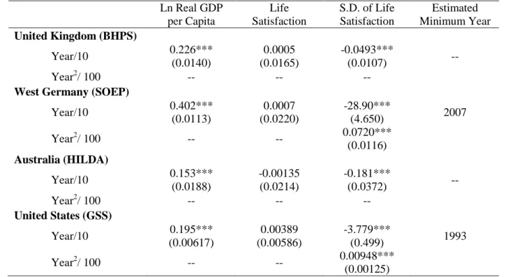
One drawback of the WVS is its small time-series dimension.3 We therefore now turn to single-country datasets, which contain many more waves of data. We use four popular long-running single-country datasets, covering the United Kingdom (BHPS), Germany (SOEP), Australia (HILDA), and the United States (GSS). We summarise the way in which happiness and GDP co-move over time in the regressions in Table 1. The first three columns refer to regressions for our three dependent variables: the log of real GDP per capita, average life satisfaction, and the standard deviation of life satisfaction. We carry out separate regressions for each of the four countries. The control variables in each regression include standard demographics (as listed in the note at the foot of the table), the year (divided by 10) and (if significant) year-squared divided by 100. We include the latter to detect non-linear movements over time. We might in particular suspect that inequality in life satisfaction in the US is U-shaped over time, following the findings of Stevenson and Wolfers (2008b) and Dutta and Foster (2013).

The results in column 1 show that real GDP per capita has trended upwards in all four countries, with no evidence of any non-linearities. Column 2 suggests that average happiness is flat in all four countries.

We are most interested in the results in column 3, which show the trend in happiness inequality. In the UK and Australia, this trend is negative and linear. However, in both the US (as previously

2_{We restrict the sample to Western countries here only to avoid cluttering the figure excessively. The same shape} appears if we include all WVS countries: the regression for the left-hand panel of Figure 2A then becomes SD(Satisfaction)=0.008***year+19.33.

(11)

9 found) and Germany there is evidence of a U-shaped relationship. Column 4 calculates the turning point in happiness inequality in these two countries. These turn out to be 1993 for the US,4 and rather later in 2007 for Germany. We will below suggest that the U-shapes in these two countries are at least partly driven by developments in income inequality.5

2.4 BHPS, SOEP, HILDA and GSS: Individual Cross-Sections

At the individual level, within each country, happiness dispersion is also smaller amongst the rich than amongst the less well-off (Figure 3): the richer seem to be more insulated against various kinds of shocks. In particular, higher income allows consumption to be protected from movements in income.6 And it is in general likely that higher income allows the hedonic impact of various life shocks (job loss, divorce, etc.) to be smoothed.

2.5 BHPS, SOEP and HILDA: Individual Panels

Figure 3 referred to pooled data. We can also use our three panel datasets (we thus drop the GSS here) to look at the same correlation within-individual. The within-individual volatility of life satisfaction over time is lower for those in higher income deciles, as illustrated in Figure 4 (where the income decile we assign to the individual in the panel data is defined as the average rounded income decile per individual over the period during which they are observed in the panel).

3_{The WVS started in 1981 and has been repeated every five years since 1990-1991. The sixth wave is currently in the} field.

4

This turning point is somewhat earlier than that in Stevenson and Wolfers (2008b) and Dutta and Foster (2013), which undoubtedly comes from our use of control variables in Table 1.

5

Analogous relations between GDP and happiness inequality are found in Eurobarometer data. We show a number of the relevant single-country graphs in Appendix A Figure 2. Happiness inequality trends downwards in eight out of nine countries as GDP trends upwards. The exception is Germany.

(12)

10

2.6 A Statistical Artefact?

All of our results so far suggest that higher income goes hand in hand with less happiness inequality. However, we may worry that this is a statistical artefact. In particular, if higher incomes make people happier, and happiness is measured using a bounded scale, then inequality will fall as more people become right-censored on the top rung of the happiness ladder. At the extreme, as everyone reports the top subjective well-being score, inequality will be zero.

A first response to this worry is that there is actually no evidence in Table 1 that higher income over time does go hand-in-hand with higher happiness. We can nonetheless directly address the changing distribution of subjective well-being via histograms of happiness at the beginning and end of the periods under consideration. This is what Clark et al. (2014) do. Their striking finding is that, as GDP grows, fewer people report the lowest happiness scores. But far from becoming more heavily populated, the top category is becoming increasingly deserted in all of the BHPS, GSS, HILDA and SOEP. As a consequence, the middle happiness categories are increasingly popular. The fall in happiness inequality then actually seems to have come from a mean-preserving contraction, as the percentage reporting the lowest happiness levels is also falling.7

A further formal test, if required, of the role of censoring comes from dropping the top and bottom scores in the panel datasets.8 The test here is to look at happiness answers in year t+1 of those who reported happiness scores of between 2 and 6 (on a 1 to 7 scale) in the BHPS data (say) at year t. All of these individuals can report either higher or lower happiness when re-interviewed in year t+1. As in Table 1, the results in Figure 3 in Appendix A show that there continues to be a trend to lower happiness inequality as GDP grows in the three panels.

7 _{In general, objective happiness is converted into reported happiness via a “reporting function”. It is possible that}

(13)

11

2.7 Well-being Domains

Is there something strange about the specific distribution of overall satisfaction scores? Figure5 suggests mostly not. We here look at the trends in inequality in various domain satisfactions. Satisfaction with health, income and job all exhibit falling inequality in the UK, Germany and Australia. As was the case for life satisfaction, the US is an outlier. Job satisfaction inequality is (slightly) falling, but not that for health and income. We suspect that income inequality may play a crucial role here: this is the topic of the next section.

3. Regression Analysis: Income Inequality and Public Goods

The results above come from analyses without any controls other than basic demographics. Can we now identify variables that help to explain the fall in happiness inequality over time? We here consider the role of income inequality and public goods. Recent years have seen rising incomes accompanied by rising income inequality9 in many countries (which we would suppose to increase happiness inequality).10 We do indeed find rising income inequality over time in the BHPS, GSS, HILDA and SOEP datasets.

At the same time, we may also reasonably expect income growth in general to produce public goods (like education, health, public infrastructure and social protection). Modern growth also comes with non-material public goods, such as lower violence and crime, greater freedom of choice in private life, political freedom, transparency and pluralism, better governance, and so on (Inglehart, 1997, and Inglehart et al., 2008). These public goods are, by definition, available to everyone (although,

operate both in the cross-section and in time series, and operate in something of the same way across countries. We arguably know only little about reporting functions, and how they may change over time.

8_{We cannot do this in the GSS, of course, as it is not panel.} 9

(14)

12 of course, their marginal benefit may differ across individuals). We then suspect that their provision will reduce happiness inequality.

The role of income inequality and public goods in determining the standard deviation of life satisfaction is explored in Table 2. The data here is the WVS and these are OLS regressions.11 The “public-good”-type variables we consider are Government expenditure, Life expectancy, the under-five Mortality rate, the Control of Corruption, Civil Liberties, Trust and Religious Fractionalisation. While we group these together under the heading “Public Goods”, they are not all 100% publicly-provided. Amongst the variables in Table 2, health is probably a publicly-provided public good, whereas something like trust is at least partly privately-produced.

We also control separately for the level of GDP per capita and income inequality by country-year. All of the explanatory variables are described in Appendix B. The four separate regressions in Table 2 are balanced, in that they are estimated only on the sample of observations with no missing values for the most complete specification (that in column 4).

The changes over time in our seven public-goods variables over our broad analysis period appear in Appendix Table 4. Government expenditure as a percentage of GDP has been on an upward trend over the past 20 years, and life expectancy has risen sharply since the early 1980s, at the same time as the under-five mortality rate has been falling. On the contrary the upward trend in trust (from the WVS) is only weak, and there is no discernible trend in the control of corruption and civil liberties. The last figure here shows the rise in income inequality since 1970, using data from the Luxembourg Income Study (LIS).

10

Becchetti et al. (2014) find that education reduces and unemployment increases happiness inequality. They however do not find any role for income inequality. Their measure of the latter is the share of the poor, which is different from ours.

(15)

13 The first column of Table 2 confirms, as expected from Figure 1, that happiness inequality does indeed fall with the log of GDP per capita.12 Column 2 then adds income inequality, as measured by the Mean Log Deviation in Income, and our measure of government expenditure. These attract insignificant coefficients, and their addition only mildly affects the estimated coefficient on log GDP per capita.13 Column 3 adds the two health variables, control of corruption and civil liberties. Their inclusion turns the coefficient on GDP per capita insignificant, while the estimated coefficients on these “public-good” variables are of the expected sign (better outcomes reduce happiness inequality). Economic growth thus seems to reduce happiness inequality because it provides public goods that tighten the distribution of subjective well-being: the correlation between GDP per capita and life expectancy, mortality and the control of corruption are all around 0.8 in absolute value, while that with civil liberties is 0.67. Last, column 4 adds measures of trust and religious fractionalisation to the regression. Neither of these is significant14 (although religious fractionalisation varies only little within countries over time, and we here include country fixed effects). Income inequality is positively correlated with happiness inequality in column (4).

Income growth would therefore seem to reduce happiness inequality because it allows for the greater provision of public goods. However, if this growth is accompanied by too large a rise in income inequality, then it is entirely possible that happiness inequality will actually rise as a result: this is arguably what we have observed in the US data above, and perhaps to a lesser extent in Germany.

12_{The errors are clustered at the country-year level here (which is the aggregation level of GDP per capita), to avoid} under-estimating the standard errors: see Moulton (1990).

13

We might worry about reverse causality, with subjective well-being affecting productivity at work, and thus income (See Ostroff, 1992, for survey analysis and Oswald et al., 2014, for an experimental approach). Our argument throughout this paper is a second-moment one, relating the level of income to the spread of the subjective well-being distribution. We actually find no relationship between average income and average well-being in our individual-country panels (see column 2 of Table 1). The only way in which movements in life satisfaction could then drive the level of income would be if the rising life satisfaction of the previously dissatisfied increases productivity more than the falling life satisfaction of the previously satisfied reduces productivity. We know of no evidence for such non-linear effects.

(16)

14

4. Additional Tests

All of our analysis above uses the standard deviation in respondents’ self-declared satisfaction as our key dispersion measure. Such a measure assumes that happiness is continuous and cardinal, with equal distances between the steps. Although such an assumption is common in the field, we have no way of knowing whether it is actually true. To be on the safe side, we have reproduced our results using the Index of Ordinal Variation (Berry and Mielke, 1992), a measure of variation specifically designed for ordinal measures.15As shown in Clark et al. (2014), the movement over time in the IOV is practically identical to that in the standard deviation of happiness, so it is perhaps unsurprising that they produce such similar results.

One common cardinal measure of dispersion is the Gini coefficient. The movements over time in the Gini coefficient of subjective well-being are depicted in Appendix Figure 5. As was the case for the standard deviation, this falls over time, with a sharp upturn towards the end of the period in the US, and a smaller upturn for West Germany. A regression such as that in column 1 of Table 2 with the Gini of well-being as the dependent variable produces a negative significant coefficient; adding the controls in column 4 renders this coefficient insignificant.

Our empirical results in Section 3 come from both repeated cross-section and panel data. One potential problem in panel data is that of panel conditioning. Landua (1992) underlined that individuals seem to become used to satisfaction scales after a while in SOEP data. He, in particular, noted a tendency away from the end values. This finding was reproduced on more recent SOEP data by Frick et al. (2006). Wooden and Li (2014) analyse HILDA data and find a clear narrowing in the dispersion of satisfaction scores over the first few waves in which the individual responds. We have

14

It is not always easy to have good measures of social capital at the cross-country level. Although trust is insignificant in this regression, some other measure of social capital may do better. The difficulty is in finding consistent measures across countries and over time.

(17)

15 checked what happens to the trend in life satisfaction when we drop the first two participation waves per individual. The results appear in Appendix Figure 6 for our three panel data sets, and continue to show a downward trend in dispersion, with again the exception of the final few years in West Germany.16

Last, it might be suspected that there is something inherent about self-reported variables, particularly in a panel-data context, which produces more homogenous responses over time. We here run a placebo test by looking at the changing standard deviation over time in other variables available in our four single-country datasets. For the BHPS, SOEP and GSS, we use self-reported interest in politics, which is measured on a one-to-four ordinal scale; in HILDA we consider the self-reported number of hours per week spent volunteering.

The results appear in Appendix A Figure 7. There is little evidence of any particular trend in the dispersion of these measures over time, and certainly no evidence of a downward trend. The shrinking dispersion of subjective well-being over time in our datasets appears to be specific to this question, rather than a general feature of self-reports.

5. Conclusions

In spite of the great U-turn that saw income inequality rise in Western countries in the 1980s, happiness inequality has notably fallen in countries that have experienced consistent income growth (but not in those that did not). Modern growth has reduced the share of both the “very unhappy” and the “perfectly happy”. The extension of public amenities may have contributed to this greater happiness homogeneity by reducing the insecurity faced by the worst-off groups in the population.

15_{Dutta and Foster (2013) also propose an ordinal measure of happiness inequality.}

(18)

16 We believe that higher national income goes hand-in-hand with a reduced spread in happiness. It can always be countered that there are potential common factors that drive both income/GDP and the inequality of happiness. One example, at the country level, might be the quality of institutions. Higher quality institutions (including educational institutions) might lead to both higher GDP and a smaller spread in happiness. Any omitted variable which explains all of our empirical findings would however have to vary across countries and within countries over time, and across individuals and within individuals over time, in the same way that income does: no obvious candidates come to mind.

The question of why the top of the happiness is increasingly deserted is perhaps a more difficult one to answer. One salient point is that the extension of public goods and government expenditure is costly, and the happier may have borne the brunt of the necessary taxation. A second explanation, which is far more difficult to test, is that growth has enlarged the world of possibilities of those previously at the top of the well-being distribution, raising their aspirations and reducing their satisfaction. Comparisons may be made not only within country, but also across countries (as suggested by Becchettiet al., 2013), and the worldwide integration of the elite is likely an integral part of globalization (Goldthorpe and McKnight, 2004). It is also possible that some of the by-products of economic growth have rendered comparisons to others easier to make and more salient. This is very likely the case with the internet. Clark and Senik (2010) show that those who have internet access at home are also more likely to report that they compare their income to others (although they do not have data on exogenous changes in internet access, for which see Lohmann, 2014). Over the course of economic growth, this dampening effect will be concentrated amongst the richer, and perhaps also amongst those who were previously the happier.

As in much of this literature, we find no evidence that economic growth has been accompanied by higher mean levels of subjective well-being. But we certainly believe that it has come along with

(19)

17 reduced happiness inequality. This new “augmented” Easterlin paradox therefore offers a somewhat brighter perspective: economic growth is a useful tool for policy-makers who care not only about average subjective well-being, but also its distribution.

(20)

18

References

Atkinson, T. Piketty, T. and Saez, E. (2011). “Top Incomes in the Long Run of History”, Journal of Economic Literature, 49, 3-71.

Becchetti, L., Castriota, S., Corrado, L., and Ricca, E. (2013). “Beyond the Joneses: Inter-country income comparisons and happiness”, Journal of Behavioral and Experimental Economics, 45, 187-195.

Becchetti, L., Massari, R., and Naticchioni, P. (2014). “The drivers of happiness inequality: suggestions for promoting social cohesion”, Oxford Economic Papers, 66, 419-442

Berry, K.J. and Mielke, P.W., Jr. (1992), “Assessment of variation in ordinal data”. Perceptual and Motor Skills, 74, 63-66.

Clark, A.E., Flèche, S., and Senik, C. (2014).“The Great Happiness Moderation”. Forthcoming in A.E. Clark and C. Senik (Eds.), Happiness and Economic Growth: Lessons from Developing Countries. Oxford: Oxford University Press.

Clark, A.E., Frijters, P., and Shields, M. (2008). “Relative Income, Happiness and Utility: An Explanation for the Easterlin Paradox and Other Puzzles”. Journal of Economic Literature, 46, 95-144.

Clark, A.E., and Senik, C. (2010). “Who compares to whom? The anatomy of income comparisons in Europe”. Economic Journal, 120, 573-594.

Dutta, I., and Foster, J. (2013). “Inequality of Happiness in the US: 1972-2010”. Review of Income and Wealth, 59, 393-415.

Easterlin, R. (1974). “Does Economic Growth Improve the Human Lot?” In P.A. David and W.B. Melvin (Eds.), Nations and Households in Economic Growth. Palo Alto: Stanford University Press.

Easterlin, R. (1995). “Will Raising the Incomes of All Increase the Happiness of All?”. Journal of Economic Behavior and Organization, 27, 35-47.

Frick, J., Goebel, J., Schechtman, E., Wagner, G., and Yitzhaki, S. (2006). “Using Analysis of Gini (ANoGi) for Detecting Whether Two Sub-Samples Represent the Same Universe: The SOEP Experience”, Sociological Methods and Research, 34, 427-468.

Goldthorpe, J. and McKnight, A. (2004). “The economic basis of social class”, LSE, Centre for Analysis of Social Exclusion, Centre for Analysis of Social Exclusion, CASE Paper 080. Heston, A., Summers, R. and Aten, B. Penn World Table Version 7.0, Center for International

Comparisons of Production, Income and Prices at the University of Pennsylvania, May 2011.

Inglehart, R. (1997). Modernization and Post-Modernization: Cultural, Economic and Political Change in 43 Societies, Princeton, NJ: Princeton University Press.

Inglehart, R., Foa, R., Peterson, C., and Welzel, C. (2008). “Development, Freedom, and Rising Happiness: A Global Perspective (1981–2007)”. Perspectives on Psychological Science, 3, 264-285.

Krueger, D. and Perri, F. (2006). “Does Income Inequality lead to Consumption Inequality?” Review of Economic Studies, 73, 163-193.

Lohmann, S. (2014). “Information Technologies and Subjective Well-being: Does the Internet Raise Material Aspirations?” University of Goettingen, mimeo.

Landua, D. (1992). “An Attempt to Classify Satisfaction Changes: Methodological and content Aspects of a Longitudinal Problem”, Social Indicators Research, 26, 221-241.

Moulton, B. (1990). “An Illustration of a Pitfall in Estimating the Effects of Aggregate Variables on Micro Units”. Review of Economics and Statistics, 72, 334-38.

(21)

19 Ostroff, C. (1992) “The relationship between satisfaction, attitudes and performance: An

organizational-level analysis”. Journal of Applied Psychology, 77, 963-974.

Oswald, A.J., Proto, E., and Sgroi, D. (2014) “Happiness and Productivity”. Journal of Labor Economics, forthcoming.

Stevenson, B., and Wolfers, J. (2008a), “Economic Growth and Subjective Well-Being: Reassessing the Easterlin Paradox”, Brookings Papers on Economic Activity, Spring, 1-102. Stevenson, B. and Wolfers, J. (2008b). “Happiness Inequality in the United States”, Journal of

Legal Studies, 37, S33-S79.

Veenhoven, R. (2005). “Inequality of Happiness in Nations”, Journal of Happiness Studies, 6, 351-355.

Wagner, G., Frick J. and Schupp J. (2007).“The German Socio-Economic Panel Study (SOEP) - Scope, Evolution and Enhancements”, Schmollers Jahrbuch, 127, 139-169.

Wooden, M., and Li, N. (2014). “Panel Conditioning and Subjective Well-being”, Social Indicators Research, 117, 235–255.

(22)

20

Figures

Figure 1. Happiness Inequality and GDP per capita. WVS Cross-Section, Last available year (2000s)

S.D. of Life Satisfaction S.D. of Life Satisfaction / Mean

Notes: These figures are based on the most recent available year for each country in the World Values Survey. Happiness inequality is measured as the standard deviation or coefficient of variation of life satisfaction per country per year. The right-hand figure above is taken from Clark et al. (2014).

(23)

21

Figure 2A. Happiness Inequality within Countries with Uninterrupted GDP Growth. WVS Panel. Selected Western countries

Note: The points show the levels of life-satisfaction inequality for countries with uninterrupted real GDP growth, over periods of at least 5 years.

Figure 2B. Happiness Inequality within Country in Countries with Falling GDP. WVS Panel.

Note: The lines show the levels of life-satisfaction inequality for countries with some periods of negative growth, over periods of at least 5 years.

(24)

22

Figure 3. Income as a Buffer Stock: The Standard Deviation of Happiness is Lower in Higher Income Deciles

United Kingdom (BHPS) West Germany (SOEP)

Australia (HILDA) United States(GSS)

Notes: Standard deviations of life satisfaction are calculated by income decile. We select people aged between 18 and 65 years old; we also drop observations corresponding to a declared income of below 500$ per year.

(25)

23

Figure 4. Income as a Buffer Stock: The Standard Deviation of Happiness within Individual over Time is Lower for Individuals in Higher Income Deciles

Australia (HILDA)

Notes: Standard deviations of life satisfaction are calculated by individual, over time and then averaged by income decile. We select people aged between 18 and 65 years old; we also drop observations corresponding to

a declared income of below 500$ per year. “Income decile” is defined as the rounded average income decile per

(26)

24

Figure 5. Trends in Satisfaction Inequality by Domain

United Kingdom (BHPS)

Health (1-7) Income (1-7) Job (1-7)

West Germany (SOEP)

Australia (HILDA)

United States (GSS)

Health (1-7) Income (1-3) Job(1-4)

Notes: We select people aged between 18 and 65 years old; we also drop observations corresponding to a declared income of below 500$ per year. GDP per capita figures are taken from Heston, Summers and Aten - the Penn World Tables.

(27)

25

Tables

Table 1. Time Trends in GDP per capita, Happiness and Happiness Inequality. Single-country Panels.

Ln Real GDP per Capita Life Satisfaction S.D. of Life Satisfaction Estimated Minimum Year United Kingdom (BHPS) Year/10 0.226*** (0.0140) 0.0005 (0.0165) -0.0493*** (0.0107) -- Year2/ 100 -- -- --

West Germany (SOEP)

Year/10 0.402*** (0.0113) 0.0007 (0.0220) -28.90*** (4.650) 2007 Year2/ 100 -- -- 0.0720*** (0.0116) Australia (HILDA) Year/10 0.153*** (0.0188) -0.00135 (0.0214) -0.181*** (0.0372) -- Year2/ 100 -- -- -- United States (GSS) Year/10 0.195*** (0.00617) 0.00389 (0.00586) -3.779*** (0.499) 1993 Year2/ 100 -- -- 0.00948*** (0.00125)

Note: Happiness and life satisfaction questions are administered consistently over time within countries for all of these surveys, although the surveys use different scales: 1-3 in the GSS, 0-10 in the SOEP and HILDA, and 1-7 in the BHPS. We select people aged between 18 and 65 years old; we also drop observations corresponding to a declared income of below 500$ per year. GDP per capita figures are taken from Heston, Summers and Aten

– the Penn World Tables. The other controls include gender, age, age-squared, marital status, labour-force status

(28)

26

Table 2. OLS Estimates of the Determinants of SD Life Satisfaction: WVS-EVS (1981 -2008) (1) (2) (5) (6) Ln GDP Per capita -0.298** (0.128) -0.240* (0.137) -0.129 (0.117) -0.127 (0.116)

Mean Log Deviation in Income 0.543* (0.329) 0.771** (0.328) 0.776** (0.354) Government Expenditure (% of GDP) 0.004 (0.004) 0.006 (0.004) 0.006 (0.004)

Life expectancy at birth -0.022*

(0.012)

-0.022* (0.013)

Mortality rate, under-5 (per 1000 live births) -0.002 (0.002) -0.002 (0.002) Control of Corruption 0.001 (0.025) 0.001 (0.025)

Limits on Civil Liberties 0.083***

(0.030) 0.083*** (0.030) Trust 0.011 (0.128) Religious Fractionalisation -0.572 (1.130) Observations 198,585 198,585 198,585 198,585 No. Countries 70 70 70 70 No. Country-year 161 161 161 161 Adjusted R2 0.896 0.899 0.910 0.910

Notes: The other controls include country fixed effects, time trends, age-category dummies, sex, labour-force status, and marital status. The errors are clustered at the country-year level. See Appendix B for the detailed variable descriptions. * significant at the 10% level, ** significant at the 5% level and *** significant at the 1% level. Weighted estimates.

(29)

27

Appendix A.

Appendix Figure 1. Happiness Inequality within Country in Growing Countries. Eurobarometer. Selected Western countries

S.D of life satisfaction

Appendix Figure 2. Single-country Trends in Income Growth and Happiness Inequality, Eurobarometer.

United Kingdom Luxembourg

(30)

28

Netherlands Italy

Belgium Ireland

Notes: Life satisfaction is administered on a 4-point scale. We select people aged between 18 and 65. GDP per capita figures are taken from Heston, Summers and Aten – the Penn World Tables. The values plotted are SD residuals by year from a regression of life satisfaction on gender, age, age-squared, marital status, employment status and education.

(31)

29

Appendix. Figure 3. The Trend in the Standard Deviation of Happiness Excluding People Who Report the Highest or Lowest Levels of Happiness

Australia (HILDA)

Note: We drop observations corresponding to people who reported being in the top or bottom life satisfaction categories one year previously.

(32)

30

Appendix. Figure 4. The Trend in the Gini Coefficient of Subjective Well-Being

(33)

31

Appendix. Figure 5. The Trend in the Standard Deviation of Happiness Excluding the First Two Years People Report Life Satisfaction

Australia (HILDA)

Note: We drop observations corresponding to the first two years in which individuals appear in the panels in question.

(34)

32

Appendix Figure 6. Placebo Variables

Interest in politics Interest in politics

Volunteering Interest in politics

Australia (HILDA) United States (GSS)

Notes: Interest in politics ranges from 1 to 4, where 1 means “very interested” and 4 “not at all interested”. Participation in volunteer work is defined as the number of hours per week.

(35)

33

Appendix B.

This paper uses the five currently available waves of the World Values Survey (WVS, 1981-2008), covering 105 countries. These include high-income, low-income and transition countries, as well as data from the ISSP and the 2002 Latinobarómetro. We also analyze individual-country surveys, such as the British Household Panel Survey (BHPS, 1996-2008), the German Socio-Economic Panel (SOEP,1 1984-2009), the American General Social Survey (GSS, 1972-2010) and the Household,

Income and Labour Dynamics in Australia survey (HILDA, 2001-2009).

The Happiness and Life Satisfaction questions were administered in the same format across all these surveys, but with different response scales: 1-3 in the GSS, 1-10 in the WVS, 0-10 in the SOEP and the Australian HILDA, 1-7 in the BHPS. The wording of the life satisfaction question in the WVS

was “All things considered, how satisfied are you with your life as a whole these days?: 1

(dissatisfied)….10(very satisfied)”. In the SOEP, it was “How satisfied are you with your life, all

things considered?”: 0 (totally unsatisfied) … 10 (totally satisfied). The BHPS survey asked “How dissatisfied or satisfied are you with your life overall?”: 1 (not satisfied at all) … 7 (completely satisfied)”. The wording of the happiness question in the GSS was “Taken all together, how would you say things are these days - would you say that you are very happy, pretty happy, or not too happy?”. We do not need to harmonize these scales, as we consider the evolution of the variance of

happiness over time within countries. The surveys cover representative samples of the population in participating countries, with an average sample size of ten to fifteen thousand respondents in each wave. We select people aged between 18 and 65 years old; we also drop observations corresponding to a declared income of below 500$ per year.

We use the American General Social Survey because it is the only long-run survey containing a happiness or life satisfaction question in the United States. However, this data is not really suited to our purpose, as only three responses are possible (very happy, pretty happy, and not too happy), making the calculation of the variance problematic. However, as the evidence initially used to suggest the Easterlin paradox partly relied on American data, and because we would like to include data from the United States, we do report the results based on this data, although they may need to be considered with some caution.

Description of the Country-level Control Variables used in Table 2

GDP per capita. GDP per capita in constant 2000 dollars (Penn World Tables)

Mean Log Deviation in Income is a measure of income inequality derived from WVS. World Bank Database (http://databank.worldbank.org/data/home.aspx)

Expenditure (% of GDP). This is cash payments for operating activities of the government in

providing goods and services. It includes compensation of employees (such as wages and salaries),

1_{See Wagner et al. (2007).}

(36)

34

interest and subsidies, grants, social benefits, and other expenses such as rent and dividends. When there is no information for some years, the first year available is used as a replacement.

Life expectancy at birth, total (years). This is given by the number of years a newborn infant would

live if prevailing patterns of mortality at the time of its birth were to stay the same throughout its life.

Mortality rate, under-5 (per 1,000 live births). This is the probability per 1,000 that a newborn

baby will die before reaching age five, if subject to current age-specific mortality rates.

Governance Indicators

Control of corruption (Transparency International). This index measures the perceived levels of

public sector corruption on a scale of 0-10, where 0 means that a country is perceived as highly corrupt and a 10 means that a country is perceived as very clean. When there is no information for some years, the first year available is used as a replacement.

Limits on Civil liberties (Freedom House). Civil Liberties contain numerical ratings between 1 and 7

for each country or territory, with 1 representing the most free and 7 the least free. Civil liberties contains information on freedom of expression and belief, associational and organizational rights, rule of law, personal autonomy and individual rights.

World Values Survey

Trust is the percentage of individuals who answer “most people can be trusted” to the question “Generally speaking, would you say that most people can be trusted or that you can’t be too careful in dealing with people?”.

Fractionalisation Data

Religious Fractionalisation comes from the fractionalisation dataset compiled by Alberto Alesina

and associates and measures the degree of religious heterogeneity in various countries. When there is no information for some years, the last year available is used as a replacement.

(37)