HAL Id: hal-01117516
https://hal.archives-ouvertes.fr/hal-01117516
Submitted on 18 Feb 2015
HAL is a multi-disciplinary open access
archive for the deposit and dissemination of
sci-entific research documents, whether they are
pub-lished or not. The documents may come from
teaching and research institutions in France or
abroad, or from public or private research centers.
L’archive ouverte pluridisciplinaire HAL, est
destinée au dépôt et à la diffusion de documents
scientifiques de niveau recherche, publiés ou non,
émanant des établissements d’enseignement et de
recherche français ou étrangers, des laboratoires
publics ou privés.
Shape Warping and Empirical Shape Statistics
Guillaume Charpiat, Olivier Faugeras, Renaud Keriven, Pierre Maurel
To cite this version:
Guillaume Charpiat, Olivier Faugeras, Renaud Keriven, Pierre Maurel. Approximations of Shape
Metrics and Application to Shape Warping and Empirical Shape Statistics.
Krim, Hamid and
Yezzi, Anthony. Statistics and Analysis of Shapes, Birkhäuser, pp.363–395, 2006, 978-0-8176-4481-9.
�10.1007/0-8176-4481-4_15�. �hal-01117516�
application to shape warping and empirical
shape statistics
Guillaume Charpiat1, Olivier Faugeras2, Renaud Keriven3, and Pierre Maurel4
1
Odyss´ee Laboratory, ENS, 45 rue d’Ulm, 75005 Paris, France Guillaume.Charpiat@ens.fr
2
Odyss´ee Laboratory, INRIA Sophia Antipolis, 2004 route des Lucioles, BP 93 06902, Sophia-Antipolis Cedex, France faugeras@sophia.inria.fr
3
Odyss´ee Laboratory, ENPC, 6 av Blaise Pascal, 77455 Marne la Vall´ee, France Renaud.Keriven@ens.fr
4
Odyss´ee Laboratory, ENS, 45 rue d’Ulm, 75005 Paris, France Pierre.Maurel@ens.fr
This chapter proposes a framework for dealing with two problems related to the analysis of shapes: the definition of the relevant set of shapes and that of defining a metric on it. Following a recent research monograph by Delfour and Zolesio [8], we consider the characteristic functions of the subsets of R2 and their distance functions. The L2 norm of the difference of characteristic functions, the L∞ and the W1,2 norms of the difference of distance functions define interesting topologies, in particular that induced by the well-known Hausdorff distance. Because of practical considerations arising from the fact that we deal with image shapes defined on finite grids of pixels we restrict our attention to subsets of R2 of positive reach in the sense of Federer [12], with smooth boundaries of bounded curvature. For this particular set of shapes we show that the three previous topologies are equivalent. The next problem we consider is that of warping a shape onto another by infinitesimal gradient descent, minimizing the corresponding distance. Because the distance function involves an inf, it is not differentiable with respect to the shape. We propose a family of smooth approximations of the distance function which are continuous with respect to the Hausdorff topology, and hence with respect to the other two topologies. We compute the corresponding Gˆateaux derivatives. They define deformation flows that can be used to warp a shape onto another by solving an initial value problem. We show several examples of this warping and prove properties of our approximations that relate to the existence of local minima. We then use this tool to produce computational definitions of the empirical mean and covariance of a set of shape examples. They yield an
analog of the notion of principal modes of variation. We illustrate them on a variety of examples.
1 Introduction
Learning shape models from examples, using them to recognize new instances of the same class of shapes are fascinating problems that have attracted the attention of many scientists for many years. Central to this problem is the no-tion of a random shape which in itself has occupied people for decades. Frechet [15] is probably one of the first mathematicians to develop some interest for the analysis of random shapes, i.e. curves. He was followed by Matheron [27] who founded with Serra the french school of mathematical morphology and by David Kendall [19, 21, 22] and his colleagues, e.g. Small [35]. In addition, and independently, a rich body of theory and practice for the statistical analysis of shapes has been developed by Bookstein [1], Dryden and Mardia [9], Carne [2], Cootes, Taylor and colleagues [5]. Except for the mostly theoretical work of Frechet and Matheron, the tools developed by these authors are very much tied to the point-wise representation of the shapes they study: objects are represented by a finite number of salient points or landmarks. This is an im-portant difference with our work which deals explicitely with curves as such, independently of their sampling or even parametrization.
In effect, our work bears more resemblance with that of several other au-thors. Like in Grenander’s theory of patterns [16, 17], we consider shapes as points of an infinite dimensional manifold but we do not model the variations of the shapes by the action of Lie groups on this manifold, except in the case of such finite-dimensional Lie groups as rigid displacements (translation and rotation) or affine transformations (including scaling). For infinite dimensional groups such as diffeomorphisms [10, 40] which smoothly change the objects’ shapes previous authors have been dependent upon the choice of parametriza-tions and origins of coordinates [43, 44, 42, 41, 28, 18]. For them, warping a shape onto another requires the construction of families of diffeomorphisms that use these parametrizations. Our approach, based upon the use of the dis-tance functions, does not require the arbitrary choice of parametrizations and origins. From our viewpoint this is already very nice in two dimensions but becomes even nicer in three dimensions and higher where finding parametriza-tions and tracking origins of coordinates can be a real problem: this is not required in our case. Another piece of related work is that of Soatto and Yezzi [36] who tackle the problem of jointly extracting and characterizing the mo-tion of a shape and its deformamo-tion. In order to do this they find inspiramo-tion in the above work on the use of diffeomorphisms and propose the use of a distance between shapes (based on the set-symmetric difference described in section 2.2). This distance poses a number of problems that we address in the same section where we propose two other distances which we believe to be more suitable.
Some of these authors have also tried to build a Riemannian structure on the set of shapes, i.e. to go from an infinitesimal metric structure to a global one. The infinitesimal structure is defined by an inner product in the tangent space (the set of normal deformation fields) and has to vary continuously from point to point, i.e. from shape to shape. The Riemannian metric is then used to compute geodesic curves between two shapes: these geodesics define a way of warping either shape onto the other. This is dealt with in the work of Trouv´e and Younes [43, 44, 40, 42, 41, 45] and, more recently, in the work of Klassen and Srivastava [24], again at the cost of working with parametrizations. The problem with these approaches, beside that of having to deal with parametrizations of the shapes, is that there exist global metric structures on the set of shapes (see section 2.2) which are useful and relevant to the problem of the comparison of shapes but that do not derive from an infinitesimal structure. Our approach can be seen as taking the problem from exactly the opposite viewpoint from the previous one: we start with a global metric on the set of shapes and build smooth functions (in effect smooth approximations of these metrics) that are dissimilarity measures, or energy functions; we then minimize these functions using techniques of the calculus of variation by computing their gradient and performing infinitesimal gradient descent: this minimization defines another way of warping either shape onto the other. In this endeavour we build on the seminal work of Delfour and Zolesio who have introduced new families of sets, complete metric topologies, and compactness theorems. This work is now available in book form [8]. The book provides a fairly broad coverage and a synthetic treatment of the field along with many new important results, examples, and constructions which have not been published elsewhere. Its full impact on image processing and robotics has yet to be fully assessed.
In this article we also revisit the problem of computing empirical statis-tics on sets of 2D shapes and propose a new approach by combining several notions such as topologies on set of shapes, calculus of variations, and some measure theory. Section 2 sets the stage and introduces some notations and tools. In particular in section 2.2 we discuss three of the main topologies that can be defined on sets of shapes and motivate the choice of two of them. In section 3 we introduce the particular set of shapes we work with in this paper, show that it has nice compactness properties and that the three topologies defined in the previous section are in fact equivalent on this set of shapes. In section 4 we introduce one of the basic tools we use for computing shape statistics, i.e., given a measure of the dissimilarity between two shapes, the curve gradient flow that is used to deform a shape into another. Having moti-vated the introduction of the measures of dissimilarity, we proceed in section 5 with the construction of classes of such measures which are based on the idea of approximating some of the shape distances that have been presented in section 2.2; we also prove the continuity of our approximations with respect to these distances and compute the corresponding curve gradient flows. This being settled, we are in a position to warp any given shape onto another by
solving the Partial Differential Equation (PDE) attached to the particular curve gradient flow. This problem is studied in section 6 where examples are also presented. In section 7.1 we use all these tools to define a mean-shape and to provide algorithms for computing it from sample shape examples. In section 7.2, we extend the notion of covariance matrix of a set of samples to that of a covariance operator of a set of sample shape examples from which the notion of principal modes of variation follows naturally.
2 Shapes and shape topologies
To define fully the notion of a shape is beyond the scope of this article in which we use a limited, i.e purely geometric, definition. It could be argued that the perceptual shape of an object also depends upon the distributiion of illumination, the reflectance and texture of its surface; these aspects are not discussed in this paper. In our context we define a shape to be a measurable subset of R2. Since we are driven by image applications we also assume that all our shapes are contained in a hold-all open bounded subset of R2 which we denote by D. The reader can think of D as the ”image”.
In the next section we will restrict our interest to a more limited set of shapes but presently this is sufficient to allow us to introduce some methods for representing shapes.
2.1 Definitions
Since, as mentioned in the introduction, we want to be independent of any particular parametrisation of the shape, we use two main ingredients, the characteristic function of a shape Ω
χΩ(x) = 1 if x∈ Ω and 0 if x /∈ Ω, and the distance function to a shape Ω
dΩ(x) = inf
y∈Ω|y − x| = infy∈Ωd(x, y) if Ω6= ∅ and +∞ if Ω = ∅. Note the important property [8, chapter 4, theorem 2.1]:
(1) dΩ1 = dΩ2 ⇐⇒ Ω1= Ω2
Also of interest is the distance function to the complement of the shape, d∁Ω and the distance function to its boundary, d∂Ω. In the case where Ω = ∂Ω and Ω is closed, we have
dΩ = d∂Ω d∁Ω = 0
We note Cd(D) the set of distance functions of nonempty sets of D. Similarly, we note Cc
subsets of D (for technical reasons which are irrelevant here, it is sufficient to consider open sets).
Another function of great interest is the oriented distance function bΩ defined as
bΩ= dΩ− d∁Ω
Note that for closed sets such that Ω = ∂Ω, one has bΩ= dΩ.
We briefly recall some well known results about these two functions. The integral of the characteristic function is equal to the measure (area) m(Ω) of
Ω: Z
Ω
χΩ(x) dx = m(Ω)
Note that this integral does not change if we add to or subtract from Ω a measurable set of Lebesgue measure 0 (also called a negligible set).
Concerning the distance functions, they are continuous, in effect Lipschitz continuous with a Lipschitz constant equal to 1 [6, 8]:
|dΩ(x)− dΩ(y)| ≤ |x − y| ∀x, y, ∈ D.
Thanks to the Rademacher theorem [11], this implies that dΩ is differentiable almost everywhere in D, i.e. outside of a negligible set, and that the magnitude of its gradient, when it exists, is less than or equal to 1
|∇dΩ(x)| ≤ 1 a.e..
The same is true of d∁Ω and bΩ (if ∂Ω 6= ∅ for the second), [8, Chapter 5, theorem 8.1].
Closely related to the various distance functions (more precisely to their gradients) are the projections associated with Ω and ∁Ω. These are also related to the notion of skeleton [8, Chapter 4 definition 3.1].
2.2 Some shape topologies
The next question we want to address is that of the definition of the similarity between two shapes. This question of similarity is closely connected to that of metrics on sets of shapes which in turn touches that of what is known as shape topologies. We now briefly review three main similarity measures between shapes which turn out to define three distances.
Characteristic functions
The similarity measure we are about to define is based upon the characteristic functions of the two shapes we want to compare. We denote by X(D) the set of characteristic functions of measurable subsets of D.
ρ2(Ω1, Ω2) = kχΩ1− χΩ2kL2 = µZ D (χΩ1(x)− χΩ2(x)) 2 dx ¶1/2
This definition also shows that this measure does not ”see” differences between two shapes that are of measure 0 (see [8, Chapter 3, Figure 3.1]) since the integral does not change if we modify the values of χΩ1 or χΩ2 over negligible
sets. In other words, this is not a distance between the two shapes Ω1 and Ω2but between their equivalence classes [Ω1]mand [Ω2]mof measurable sets. Given a measurable subset Ω of D, we define its equivalence class [Ω]m as [Ω]m={Ω′|Ω′ is measurable and Ω ∆ Ω′ is negligible}, where Ω ∆ Ω′ is the symmetric difference
Ω∆Ω′ = ∁ΩΩ′∪ ∁Ω′Ω
The proof that this defines a distance follows from the fact that the L2 norm defines a distance over the set of equivalence classes of square integrable functions (see e.g. [32, 11]).
This is nice and one has even more ([8, Chapter 3, Theorem 2.1]: the set X(D) is closed and bounded in L2(D) and ρ
2(·, ·) defines a complete metric structure on the set of equivalence classes of measurable subsets of D. Note that ρ2 is closely related to the symmetric difference:
ρ2(Ω1, Ω2) = m(Ω1∆ Ω2)
1 2
The completeness is important in applications: any Cauchy sequence of char-acteristic functions{χΩn} converges for this distance to a characteristic
func-tion χΩ of a limit set Ω. Unfortunately in applications not all sequences are Cauchy sequences, for example the minimizing sequences of the energy func-tions defined in section 5, and one often requires more, i.e. that any sequence of characteristic functions contains a subsequence that converges to a charac-teristic function. This stronger property, called compactness, is not satisfied by X(D) (see [8, Chapter 3]).
Distance functions
We therefore turn ourselves toward a different similarity measure which is based upon the distance function to a shape. As in the case of characteristic functions, we define equivalent sets and say that two subsets Ω1and Ω2 of D are equivalent iff Ω1= Ω2. We note [Ω]d the corresponding equivalence class of Ω. LetT (D) be the set of these equivalence classes. The application
[Ω]d→ dΩ T (D) → Cd(D)⊂ C(D)
is injective according to (1). We can therefore identify the set Cd(D) of dis-tance functions to sets of D with the just defined set of equivalence classes of sets. Since Cd(D) is a subset of the set C(D) of continuous functions on D, a Banach space5 when endowed with the norm
5
kfkC(D)= sup x∈D|f(x)|, it can be shown (e.g. [8]), that the similarity measure (2) ρ([Ω1]d, [Ω2]d) = kdΩ1− dΩ2kC(D) = sup
x∈D|dΩ1
(x)− dΩ2(x)|,
is a distance on the set of equivalence classes of sets which induces on this set a complete metric. Moreover, because we have assumed D bounded, the corresponding topology is identical to the one induced by the well-known Hausdorff metric (see [27, 33, 8])
(3) ρH([Ω1]d, [Ω2]d) = max ½ sup x∈Ω2 dΩ1(x), sup x∈Ω1 dΩ2(x) ¾
In fact we have even more than the identity of the two topologies, see [8, Chapter 4, Theorem 2.2]:
Proposition 1. If the hold-all set D is bounded ρ = ρH.
An important improvement with respect to the situation in the previous section is the (see [8, Chapter 4, Theorem 2.2])
Theorem 2. The set Cd(D) is compact in the set C(D) for the topology defined by the Hausdorff distance.
In particular, from any sequence {dΩn} of distance functions to sets Ωn one
can extract a sequence converging toward the distance function dΩ to a subset Ω of D.
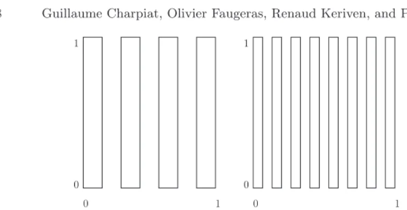
It would appear that we have reached an interesting stage and that the Hausdorff distance is what we want to measure shape similarities. Unfortu-nately this is not so because the convergence of areas and perimeters is lost in the Hausdorff metric, as shown in the following example taken from [8, Chapter 4, Example 4.1 and Figure 4.3]
Consider the sequence{Ωn} of sets in the open square ] − 1, 2[2: Ωn={(x, y) ∈ D :
2k 2n ≤ x ≤
2k + 1
2n , 0≤ k < n}
Figure 1 shows the sets Ω4 and Ω8. This defines n vertical stripes of equal width 1/2n each distant of 1/2n. It is easy to verify that, for all n ≥ 1, m(Ωn) = 1/2 and|∂Ωn| = 2n + 1. Moreover, if S is the unit square [0, 1]2, for all x∈ S, dΩn(x)≤ 1/4n, hence dΩn → dS in C(D). The sequence {Ωn}
converges to S for the Hausdorff distance but since m(Ωn) = m(Ωn) = 1/2 9 1 = m(S), χΩn 9 χS in L
2(D) and hence we do not have convergence for the ρ2 topology. Note also that|∂Ωn| = 2n + 1 9 |∂S| = 4.
0 1 0 1 0 1 0 1
Fig. 1.Two shapes in the sequence {Ωn}, see text: (left) Ω4 and (right), Ω8.
Distance functions and their gradients
In order to recover continuity of the area one can proceed as follows. If we recall that the gradient of a distance function is of magnitude equal to 1 except on a subset of measure 0 of D, one concludes that it is square integrable on D. Hence the distance functions and their gradients are square-integrable, they belong to the Sobolev space W1,2(D), a Banach space for the vector norm
kf − gkW1,2(D)=kf − gkL2(D)+k∇f − ∇gkL2(D),
where L2(D) = L2(D)× L2(D). This defines a similarity measure for two shapes
ρD([Ω1]d, [Ω2]d) = kdΩ1− dΩ2kW1,2(D)
which turns out to define a complete metric structure on T (D). The corre-sponding topology is called the W1,2-topology. For this metric, the set C
d(D) of distance functions is closed in W1,2(D), and the mapping
dΩ → χΩ= 1− |∇dΩ| : Cd(D)⊂ W1,2(D)→ L2(D) is ”Lipschitz continuous”:
(4) kχΩ1− χΩ2kL2(D)≤ k∇dΩ1− ∇dΩ2kL2(D) ≤ kdΩ1− dΩ2kW1,2(D),
which indeed shows that areas are continuous for the W1,2-topology, see [8, Chapter 4, Theorem 4.1].
Cd(D) is not compact for this topology but a subset of it of great practical interest is, see section 3.
3 The set S of all shapes and its properties
We now have all the necessary ingredients to be more precise in the definition of shapes.
3.1 The set of all shapes
We restrict ourselves to sets of D with compact boundary and consider three different sets of shapes. The first one is adapted from [8, Chapter 4, definition 5.1]:
Definition 3 (Set DZ of sets of bounded curvature). The set DZ of sets of bounded curvature contains those subsets Ω of D, Ω, ∁Ω 6= ∅ such that ∇dΩ and∇d∁Ω are in BV (D)2, where BV (D) is the set of functions of bounded variations.
This is a large set (too large for our applications) which we use as a ”frame of reference”.DZ was introduced by Delfour and Zol´esio [6, 7] and contains the setsF and C2introduced below. For technical reasons related to compactness properties (see section 3.2) we consider the following subset ofDZ.
Definition 4 (Set DZ0). The setDZ0 is the subset of DZ such that there exists c0> 0 such that for all Ω∈ DZ0,
kD2dΩkM1(D)≤ c0 andkD2d∁ΩkM1(D)≤ c0
M1(D) is the set of bounded measures on D and
kD2dΩkM1(D) is defined as
follows. Let Φ be a 2× 2 matrix of functions in C1(D), we have kD2dΩkM1(D)= sup Φ∈C1(D)2×2, kΦkC≤1 ¯ ¯ ¯ ¯ Z D∇d Ω· divΦ dx ¯ ¯ ¯ ¯, where kΦkC= sup x∈D|Φ(x)|R 2×2, and
divΦ = [divΦ1, divΦ2], where Φi, i = 1, 2 are the row vectors of the matrix Φ.
The setDZ0has the following property (see [8, Chapter 4, Theorem 5.2])
Proposition 5. Any Ω∈ DZ0 has a finite perimeter upper-bounded by 2c0. We next introduce three related sets of shapes.
Definition 6 (Sets of smooth shapes). The setC0(resp.C1,C2) of smooth shapes is the set of subsets of D whose boundary is non-empty and can be lo-cally represented as the epigraph of a C0(resp. C1, C2) function. One further distinguishes the setsCc
i andCio, i = 0, 1, 2 of subsets whose boundary is closed and open, respectively.
Note that this implies that the boundary is a simple regular curve (hence compact) since otherwise it cannot be represented as the epigraph of a C1 (resp. C2) function in the vicinity of a multiple point. Also note that
C2 ⊂ C1⊂ DZ ([6, 7]).
Definition 7 (Set F of shapes of positive reach). A nonempty subset Ω of D is said to have positive reach if there exists h > 0 such that ΠΩ(x) is a singleton for every x∈ Uh(Ω). The maximum h for which the property holds is called the reach of Ω and is noted reach(Ω).
We will also be interested in the subsets, called h0-Federer’s sets and noted Fh0, h0> 0, ofF which contain all Federer’s sets Ω such that reach(Ω) ≥ h0.
Note thatCi, i = 1, 2⊂ F but Ci6⊂ Fh0.
We are now ready to define the set of shapes of interest.
Definition 8 (Set of all shapes). The set, notedS, of all shapes (of interest) is the subset of C2 whose elements are also h0-Federer’s sets for a given and fixed h0> 0.
Sd=ef C2∩ Fh0
This set contains the two subsets Sc and
So obtained by considering Cc
2 and Co
2, respectively.
Note thatS ⊂ DZ. Note also that the curvature of ∂Ω is well defined and upperbounded by 1/h0, noted κ0. Hence, c0 in definition 4 can be chosen in such a way thatS ⊂ DZ0.
Ω ∂Ω Ω = ∂Ω d > h0 d > h0 κ≤ κ0= 1 h0
Fig. 2. Examples of admissible shapes: a simple, closed, regular curve (left); a simple, open regular curve (right). In both cases the curvature is upperbounded by κ0and the pinch distance is larger than h0.
At this point, we can represent regular (i.e. C2) simple curves with and
without boundaries that do not curve or pinch too much (in the sense of κ0
and h0, see figure 2.
There are two reasons why we choose S as our frame of reference. The
first one is because our implementations work with discrete objects defined on an underlying discrete square grid of pixels. As a result we are not able
to describe details smaller than the distance between two pixels. This is our unit and h0 is chosen to be smaller than or equal to it. The second reason is that S is included in DZ0 which, as shown in section 3.2, is compact. This will turn out to be important when minimizing shape functionals.
The question of the deformation of a shape by an element of a group of transformations could be raised at this point. What we have in mind here is the question of deciding whether a square and the same square rotated by 45 degrees are the same shape. There is no real answer to this question, more precisely the answer depends on the application. Note that the group in question can be finite dimensional, as in the case of the Euclidean and affine groups which are the most common in applications, or infinite dimensional. In this work we will, for the most part, not consider the action of groups of transformations on shapes.
3.2 Compactness properties
Interestingly enough, the definition of the setDZ0(definition 4) implies that it is compact for all three topologies. This is the result of the following theorem whose proof can be found in [8, Chapter 4, Theorems 8.2, 8.3].
Theorem 9. Let D be a nonempty bounded regular6 open subset of R2 and DZ the set defined in definition 3. The embedding
BC(D) ={dΩ ∈ Cd(D)∩ Cdc(D) :∇dΩ,∇d∁Ω ∈ BV (D)2} → W1,2(D), is compact.
This means that for any bounded sequence{Ωn}, ∅ 6= Ωn of elements of DZ, i.e. for any sequence of DZ0, there exists a set Ω6= ∅ of DZ such that there exists a subsequence Ωnk such that
dΩnk → dΩ and d∁Ωnk → d∁Ω in W1,2(D).
Since bΩ = dΩ− d∁Ω, we also have the convergence of bΩnk to bΩ, and since the mapping bΩ → |bΩ| = d∂Ω is continuous in W1,2(D) (see [8, Chapter 5, Theorem 5.1 (iv)]), we also have the convergence of d∂Ωnk to d∂Ω. The convergence for the ρ2 distance follows from equation (4):
χΩnk → χΩ in L2(D),
and the convergence for the Hausdorff distance follows from theorem 2, taking subsequences if necessary.
In other words, the setDZ0 is compact for the topologies defined by the ρ2, Hausdorff and W1,2 distances.
Note that, even thoughS ⊂ DZ0, this does not imply that it is compact for either one of these three topologies. But it does imply that its closure S for each of these topologies is compact in the compact setDZ0.
6
Regular means uniformly Lipschitzian in the sense of [8, Chapter 2, Definition 5.1].
3.3 Comparison between the three topologies on S
The three topologies we have considered turn out to be closely related onS. This is summarized in the following
Theorem 10. The three topologies defined by the three distances ρ2, ρD and ρH are equivalent onSc. The two topologies defined by ρD and ρH are equiv-alent on So.
This means that, for example, given a set Ω of Sc, a sequence
{Ωn} of elements ofSc converging toward Ω
∈ Sc for any of the three distances ρ 2, ρ (ρH) and ρDalso converges toward the same Ω for the other two distances.
We refer to [3] for the proof of this theorem.
An interesting and practically important consequence of this theorem is the following. Consider the setS, included in DZ0, and its closureS for any one of the three topologies of interest.S is a closed subset of the compact metric space DZ0 and is therefore compact as well. Given a continuous function f :S → R we consider its lower semi-continuous (l.s.c.) envelope f defined on S as follows
f (x) = ½
f (x) if x∈ S lim infy→x, y∈Sf (y) The useful result for us is summarized in the
Proposition 11. f is l.s.c. inS and therefore has at least a minimum in S. Proof. In a metric space E, a real function f is said to be l.s.c. if and only if
f (x)≤ lim infy→x f (y) ∀x ∈ E.
Therefore f is l.s.c. by construction. The existence of minimum of an l.s.c. function defined on a compact metric space is well-known (see e.g. [4, 11]) and will be needed later to prove that some of our minimization problems are well-posed.
4 Deforming shapes
The problem of continuously deforming a shape so that it turns into another is central to this paper. The reasons for this will become more clear in the sequel. Let us just mention here that it can be seen as an instance of the warping problem: given two shapes Ω1 and Ω2, how do I deform Ω1 onto Ω2? The applications in the field of medical image processing and analysis are immense (see for example [39, 38]). It can also be seen as an instance of the famous (in computer vision) correspondence problem: given two shapes Ω1 and Ω2, how do I find the corresponding point P2 in Ω2 of a given point P1in Ω1? Note that a solution of the warping problem provides a solution of
the correspondence problem if we can track the evolution of any given point during the smooth deformation of the first shape onto the second.
In order to make things more quantitative, we assume that we are given a function E :C0×C0→ R+, called the Energy, which is continuous onS ×S for one of the shape topologies of interest. This Energy can also be thought of as a measure of the dissimilarity between the two shapes. By smooth, we mean that it is continuous with respect to this topology and that its derivatives are well-defined in a sense we now make more precise.
We first need the notion of a normal deformation flow of a curve Γ inS. This is a smooth (i.e. C0) function β : [0, 1]
→ R (when Γ ∈ So, one further requires that β(0) = β(1)). Let Γ : [0, 1] → R2 be a parameterization of Γ , n(p) the unit normal at the point Γ (p) of Γ ; the normal deformation flow β associates the point Γ (p) + β(p)n(p) to Γ (p). The resulting shape is noted Γ + β, where β = βn. There is no guarantee that Γ + β is still a shape inS in general but if β is C0and ε is small enough, Γ + β is in
C0. Given two shapes Γ and Γ0, the corresponding Energy E(Γ, Γ0), and a normal deformation flow β of Γ , the Energy E(Γ + εβ, Γ0)is now well-defined for ε sufficiently small. The derivative of E(Γ, Γ0) with respect to Γ in the direction of the flow β is then defined, when it exists, as
(5) GΓ(E(Γ, Γ0), β) = lim ε→0
E(Γ + εβ, Γ0)− E(Γ, Γ0) ε
This kind of derivative is also known as a Gˆateaux semi-derivative. In our case the function β → GΓ(E(Γ, Γ0), β) is linear and continuous (it is then called a Gˆateaux derivative) and defines a continuous linear form on the vector space of normal deformation flows of Γ . This is a vector subspace of the Hilbert space L2(Γ ) with the usual Hilbert product
hβ1, β2i = |Γ |1 RΓ β1β2= 1
|Γ | R
Γβ1(x)β2(x) dΓ (x), where |Γ | is the length of Γ . Given such an inner product, we can apply Riesz’s representation theorem [32] to the Gˆateaux derivativeGΓ(E(Γ, Γ0), β): There exists a deformation flow, noted∇E(Γ, Γ0), such that
GΓ(E(Γ, Γ0), β) =h∇E(Γ, Γ0), βi. This flow is called the gradient of E(Γ, Γ0).
We now return to the initial problem of smoothly deforming a curve Γ1 onto a curve Γ2. We can state it as that of defining a family Γ (t), t ≥ 0 of shapes such that Γ (0) = Γ1, Γ (T ) = Γ2 for some T > 0 and for each value of t ≥ 0 the deformation flow of the current shape Γ (t) is equal to minus the gradient ∇E(Γ, Γ2) defined previously. This is equivalent to solving the following PDE
Γt =−∇E(Γ, Γ2)n (6)
Γ (0) = Γ1
In this paper we do not address the question of the existence of solutions to (6).
Natural candidates for the Energy function E are the distances defined in section 2.2. The problem we are faced with is that none of these distances are Gˆateaux differentiable. This is why the next section is devoted to the definition of smooth approximations of some of them.
5 How to approximate shape distances
The goal of this section is to provide smooth approximations of some of these distances, i.e. that admit Gˆateaux derivatives. We start with some notations. 5.1 Averages
Let Γ be a given curve inC1and consider an integrable function f : Γ → Rn. We denote byhfiΓ the average of f along the curve Γ :
(7) hfiΓ = 1 |Γ | Z Γ f = 1 |Γ | Z Γ f (x) dΓ (x)
For real positive integrable functions f , and for any continuous strictly monotonous (hence one to one) function ϕ from R+ or R+∗ to R+ we will also need the ϕ-average of f along Γ which we define as
(8) hfiϕΓ = ϕ−1 µ 1 |Γ | Z Γ ϕ◦ f ¶ = ϕ−1 µ 1 |Γ | Z Γ ϕ(f (x)) dΓ (x) 
Note that ϕ−1 is also strictly monotonous and continous from R+ to R+ or R+∗. Also note that the unit of the ϕ-average of f is the same as that of f , thanks to the normalization by|Γ |.
The discrete version of the ϕ-average is also useful: let ai, i = 1, . . . , n be n positive numbers, we note
(9) ha1,· · · , aniϕ= ϕ−1 Ã 1 n n X i=1 ϕ(ai) ! , their ϕ-average.
5.2 Approximations of the Hausdorff distance
We now build a series of smooth approximations of the Hausdorff distance ρH(Γ, Γ′) of two shapes Γ and Γ′. According to (3) we have to consider the functions dΓ′ : Γ → R+ and dΓ : Γ′ → R+. Let us focus on the second one.
Since dΓ is Lipschitz continuous on the bounded hold-all set D it is certainly integrable on the compact set Γ′ and we have [32, Chapter 3, problem 4]
(10) lim β→+∞ µ 1 |Γ′| Z Γ′ dβΓ(x′) dΓ′(x′) ¶β1 = sup x′∈Γ′ dΓ(x′).
Moreover, the function R+
→ R+ defined by β →³ 1 |Γ′| R Γ′d β Γ(x′) dΓ′(x′) ´β1
is monotonously increasing [32, Chapter 3, problem 5]. Similar properties hold for dΓ′.
If we note pβthe function R+→ R+defined by pβ(x) = xβ we can rewrite (10) lim β→+∞hdΓi pβ Γ′ = sup x′∈Γ′ dΓ(x′).
hdΓipΓβ′is therefore a monotonically increasing approximation of supx′∈Γ′dΓ(x′).
We go one step further and approximate dΓ′(x).
Consider a continuous strictly monotonously decreasing function ϕ : R+ → R+∗. Because ϕ is strictly monotonously decreasing
sup x′∈Γ′ ϕ(d(x, x′)) = ϕ( inf x′∈Γ′d(x, x ′)) = ϕ(d Γ′(x)), and moreover lim α→+∞ µ 1 |Γ′| Z Γ′ ϕα(d(x, x′)) dΓ′(x′) ¶α1 = sup x′∈Γ′ ϕ(d(x, x′)).
Because ϕ is continuous and strictly monotonously decreasing, it is one to one and ϕ−1 is strictly monotonously decreasing and continuous. Therefore
dΓ′(x) = lim α→+∞ϕ −1 õ 1 |Γ′| Z Γ′ ϕα(d(x, x′)) dΓ′(x′) ¶α1!
We can simplify this equation by introducing the function ϕα= pα◦ ϕ:
(11) dΓ′(x) = lim
α→+∞hd(x, ·)i ϕα
Γ′
Any α > 0 provides us with an approximation, noted ˜dΓ′, of dΓ′:
(12) d˜Γ′(x) =hd(x, ·)iϕα
Γ′
We have a similar expression for ˜dΓ. Note that because ³|Γ1′|
R Γ′ ϕ
α(d(x, x′)) dΓ′(x′)´
1 α
increases with α to-ward its limit supx′ϕ(d(x, x′)) = ϕ(dΓ′(x)), ϕ−1
µ³ 1 |Γ′| R Γ′ ϕ α(d(x, x′)) dΓ′(x′)´ 1 α
decreases with α toward its limit dΓ′(x).
ϕ1(z) = 1 z + ε ε > 0, z≥ 0 ϕ2(z) = µ exp(−λz) µ, λ > 0, z ≥ 0 ϕ3(z) = 1 √ 2πσ2exp(− z2 2σ2) σ > 0, z≥ 0 Putting all this together we have the following result
sup x∈Γ dΓ′(x) = lim α, β→+∞hhd(·, ·)i ϕα Γ′i pβ Γ sup x∈Γ′ dΓ(x) = lim α, β→+∞hhd(·, ·)i ϕα Γ i pβ Γ′
Any positive values of α and β yield approximations of supx∈Γ dΓ′(x) and
supx∈Γ′ dΓ(x).
The last point to address is the max that appears in the definition of the Hausdorff distance. We use (9), choose ϕ = pγ and note that, for a1 and a2 positive,
lim
γ→+∞ha1, a2i
pγ= max(a
1, a2).
This yields the following expression for the Hausdorff distance between two shapes Γ and Γ′ ρH(Γ, Γ′) = lim α, β, γ→+∞hhd(·, ·)i ϕα Γ′i pβ Γ ,hhd(·, ·)i ϕα Γ i pβ Γ′ ®pγ
This equation is symmetric and yields approximations ˜ρH of the Hausdorff distance for all positive values of α, β and γ:
(13) ρ˜H(Γ, Γ′) =hhd(·, ·)iϕΓα′i pβ Γ , hhd(·, ·)i ϕα Γ i pβ Γ′ ®pγ
This approximation is ”nice” in several ways, the first one being the obvious one, stated in the following
Proposition 12. For each triplet (α, β, γ) in (R+∗)3 the function ˜ρ H:S × S → R+ defined by equation (13) is continuous for the Hausdorff topology.
The complete proof of this proposition can be found in [3]. 5.3 Computing the gradient of the approximation to the Hausdorff distance
We now proceed with showing that the approximation ˜ρH(Γ, Γ0) of the Haus-dorff distance ρH(Γ, Γ0) is differentiable with respect to Γ and compute its gradient ∇ ˜ρH(Γ, Γ0), in the sense of section 4. To simplify notations we rewrite (13) as (14) ρ˜H(Γ, Γ0) = D hd(·, ·)iϕ Γ0 ®ψ Γ,hhd(·, ·)i ϕ Γi ψ Γ0 Eθ ,
Proposition 13. The gradient of ˜ρH(Γ, Γ0) at any point y of Γ is given by (15) ∇˜ρH(Γ, Γ0)(y) = 1 θ′(˜ρ H(Γ, Γ0)) (α(y)κ(y) + β(y)) ,
where κ(y) is the curvature of Γ at y, the functions α(y) and β(y) are given by (16) α(y) = ν Z Γ0 ψ′ ϕ′ (hd(x, ·)i ϕ Γ) [ ϕ◦ hd(x, ·)i ϕ Γ − ϕ ◦ d(x, y) ] dΓ0(x) +|Γ0|η h ψ³hd(·, ·)iϕΓ 0 ®ψ Γ ´ − ψ¡hd(·, y)iϕΓ0 ¢i , (17) β(y) = Z Γ0 ϕ′◦d(x, y) · νψ ′ ϕ′ (hd(x, ·)i ϕ Γ) + η ψ′ ϕ′ ¡hd(·, y)i ϕ Γ0 ¢ ¸ y − x d(x, y)·n(y) dΓ0(x), where ν = 1 |Γ | |Γ0| θ′ ψ′ ³ hhd(·, ·)iϕΓi ψ Γ0 ´ and η = 1 |Γ | |Γ0| θ′ ψ′ ³ hd(·, ·)iϕΓ0 ®ψ Γ ´ . Note that the function β(y) is well-defined even if y belongs to Γ0 since the term d(x,y)y−x is of unit norm.
The first two terms of the gradient show explicitely that minimizing the energy implies homogenizing the distance to Γ0 along the curve Γ , that is to say the algorithm will take care in priority of the points of Γ which are the furthest from Γ0.
Also note that the expression of the gradient in proposition 13 still stands when Γ and Γ0 are two surfaces (embedded in R3), if κ stands for the mean curvature.
5.4 Other alternatives related to the Hausdorff distance
There exist several alternatives to the method presented in the previous sec-tions if we use ρ (equation (2)) rather than ρH (equation (3)) to define the Hausdorff distance. A first alternative is to use the following approximation
˜
ρ(Γ, Γ′) =h|dΓ − dΓ′|ipα
D,
where the bracketh f(.) iϕDis defined the obvious way for any integrable func-tion f : D→ R+ h f iϕD= ϕ−1 µ 1 m(D) Z D ϕ(f (x)) dx ¶ ,
and which can be minimized, as in section 5.6, with respect to dΓ. A second alternative is to approximate ρ using:
(18) ρ(Γ, Γ˜ ′) =h|hd(·, ·)iϕβ Γ′ − hd(·, ·)i ϕβ Γ |i pα D,
and to compute is derivative with respect to Γ as we did in the previous section for ˜ρH.
5.5 Approximations to the W1,2 norm and computation of their gradient
The previous results can be used to construct approximations ˜ρD to the dis-tance ρD defined in section 2.2:
(19) ρ˜D(Γ1, Γ2) =k ˜dΓ1− ˜dΓ2kW1,2(D),
where ˜dΓi, i = 1, 2 is obtained from (12).
This approximation is also ”nice” in the usual way and we have the Proposition 14. For each α in R+∗ the function ˜ρ
D : S × S → R+ is continuous for the W1,2 topology.
Its proof is left to the reader.
The gradient∇˜ρD(Γ, Γ0), of our approximation ˜ρD(Γ, Γ0) of the distance ρD(Γ, Γ0) given by (19) in the sense of section 4 can be computed. The inter-ested reader is referred to the appendix of [3]. We simply state the result in the
Proposition 15. The gradient of ˜ρD(Γ, Γ0) at any point y of Γ is given by (20) ∇˜ρD(Γ, Γ0)(y) = Z D · B(x, y) µ C1(x)− ϕ” ϕ′( ˜dΓ(x)) ³ C2(x)· ∇ ˜dΓ(x) ´¶ + C2(x)· ∇B(x, y) ¸ dx, where
B(x, y) = κ(y) (hϕ ◦ d(x, ·)iΓ − ϕ ◦ d(x, y)) + ϕ′(d(x, y)) y− x d(x, y)· n(y), κ(y) is the curvature of Γ at y,
C1(x) = 1 |Γ | ϕ′( ˜d Γ(x)) k ˜dΓ − ˜dΓ0k −1 L2(D) ³ ˜dΓ(x)− ˜dΓ0)(x) ´ , and C2(x) = 1 |Γ | ϕ′( ˜d Γ(x)) k∇( ˜dΓ − ˜dΓ0)k −1 L2(D) ∇( ˜dΓ − ˜dΓ0)(x),
5.6 Direct minimization of the W1,2 norm
An alternative to the method presented in the previous section is to evolve not the curve Γ but its distance function dΓ. Minimizing ρD(Γ, Γ0) with respect to dΓ implies computing the corresponding Euler-Lagrange equation EL. The reader will verify that the result is
(21) EL = dΓ − dΓ0 kdΓ − dΓ0kL2(D) − div µ ∇ (dΓ− dΓ0) k∇(dΓ − dΓ0)kL2(D)) 
To simplify notations we now use d instead of dΓ. The problem of warping Γ1 onto Γ0 is then transformed into the problem of solving the following PDE
dt=−EL d(0,·) = dΓ1(·).
The problem that this PDE does not preserve the fact that d is a distance function is alleviated by ”reprojecting” at each iteration the current function d onto the set of distance functions by running a few iterations of the ”standard” restoration PDE [37]
dt= (1− |∇d|)sign(d0) d(0,·) = d0
6 Application to curve evolutions: Hausdorff warping
In this section we show a number of examples of solving equation (6) with the gradient given by equation (15). Our hope is that, starting from Γ1, we will follow the gradient (15) and smoothly converge to the curve Γ2where the min-imum of ˜ρHis attained. Let us examine more closely these assumptions. First, it is clear from the expression (13) of ˜ρH that in general ˜ρH(Γ, Γ )6= 0, which implies in particular that ˜ρH, unlike ρH, is not a distance. But worse things can happen: there may exist a shape Γ′ such that ˜ρ
H(Γ, Γ′) is strictly less than ˜
ρH(Γ, Γ ) or there may not exist any minima for the function Γ → ˜ρH(Γ, Γ′)! This sounds like the end of our attempt to warp a shape onto another using an approximation of the Hausdorff distance. But things turn out not to be so bad. First, the existence of a minimum is guaranteed by proposition 12 which says that ˜ρH is continuous onS for the Hausdorff topology, theorem 9 which says thatDZ0 is compact for this topology, and proposition 11 which tells us that the l.s.c. extension of ˜ρH(·, Γ ) has a minimum in the closure S of S in DZ0.
We show in the next section that phenomena like the one described above are for all practical matters ”invisible” since confined to an arbitrarily small Hausdorff ball centered at Γ .
6.1 Quality of the approximation ˜ρH of ρH
In this section we make more precise the idea that ˜ρHcan be made arbitrarily close to ρH. Because of the form of (14) we seek upper and lower bounds of such quantities as hfiψΓ, where f is a continuous real function defined on Γ . We note fmin the minimum value of f on Γ .
The expression hfiψΓ = ψ −1 µ 1 |Γ | Z Γ ψ◦ f ¶ ,
yields, if ψ is strictly increasing, and if f > fmoy on a set F of the curve Γ , of
length|F | (6 |Γ |): hfiψΓ = ψ −1 Ã 1 |Γ | Z F ψ◦ f + 1 |Γ | Z Γ \F ψ◦ f ! > ψ−1µ |F | |Γ |ψ◦ fmoy+ |Γ | − |F | |Γ | ψ◦ fmin ¶ > ψ−1µ |F | |Γ |ψ◦ fmoy 
To analyse this lower bound, we introduce the following notation. Given ∆, α > 0, we noteP(∆, α) the following property:
P(∆, α) : ∀x ∈ R+, ∆ψ(x) > ψ(αx) This property is satisfied for example for ψ(x) = xβ, β
≥ 0. The best pairs (∆, α) verifyingP are such that ∆ = αβ. In the sequel, we consider a function ψ which satisfies:
∀∆ ∈]0; 1[, ∃α ∈]0; 1[, P(∆, α), and, conversely,
∀α ∈]0; 1[, ∃∆ ∈]0; 1[, P(∆, α)
Then for ∆ψ= |F ||Γ | and a corresponding αψ such thatP(∆ψ, αψ) is satis-fied, we have
hfiψΓ > ψ−1(∆ψψ(fmoy)) > αψ fmoy
and deduce from that kind of considerations the following property (see complete proof in [3]):
Proposition 16. ρ˜H(Γ, Γ′) has the following upper and lower bounds (22) αθαψ(ρH(Γ, Γ′)−∆ψ|Γ | + |Γ ′ | 2 )≤ ˜ρH(Γ, Γ ′) ≤ αϕ(ρH(Γ, Γ′)+∆ϕ|Γ | + |Γ ′ | 2 ). where αθ, αψand αϕare constants depending on functions θ, ψ and ϕ and can be set arbitrarily close to 1 with a good choice of these functions, while ∆ψand ∆ϕare positive constants depending on functions ψ and ϕ and can be set arbitrarily close to 0 in the same time. Consequently, the approximation
˜
ρH(Γ, Γ′) of ρH(Γ, Γ′) can be arbitrarily accurate.
We can now characterize the shapes Γ and Γ′ such that (23) ρ˜H(Γ, Γ′) < ˜ρH(Γ, Γ ).
Theorem 17. The condition (23) is equivalent (see [3] again) to ρH(Γ, Γ′) < 4c0∆,
where the constant c0 is defined in definition 4 and theorem 5, and ∆ = max(∆ψ, ∆ϕ).
From this we conclude that, since ∆ can be made arbitrarily close to 0, and the length of shapes is bounded, strange phenomena such as a shape Γ′ closer to a shape Γ than Γ itself (in the sense of ˜ρH) cannot occur or rather will be ”invisible” to our algorithms.
6.2 Applying the theory
In practice, the Energy that we minimize is not ˜ρH but in fact a ”regular-ized” version obtained by combining ˜ρHwith a term EL which depends upon the lengths of the two curves. A natural candidate for EL is max(|Γ |, |Γ′|) since it acts only if|Γ | becomes larger than |Γ′
|, thereby avoiding undesirable oscillations. To obtain smoothness, we approximate the max with a Ψ -average: (24) EL(|Γ |, |Γ′|) = h|Γ |, |Γ′|i
Ψ
We know that the function Γ → |Γ | is in general l.s.c.. It is in fact continuous on S (see the proof of proposition 12) and takes its values in the interval [0, 2c0], hence
Proposition 18. The function S → R+ given by Γ → E
L(Γ, Γ′) is contin-uous for the Hausdorff topology.
Proof. It is clear since EL is a combination of continuous functions.
We combine EL with ˜ρH the expected way, i.e. by computing their ˜Ψ average so that the final energy is
(25) E(Γ, Γ′) =h˜ρH(Γ, Γ′), EL(|Γ |, |Γ′|)i ˜ Ψ
The function E :S × S → R+ is continuous for the Hausdorff metric because of propositions 12 and 18 and therefore
Proposition 19. The function Γ → E(Γ, Γ′) defined on the set of shapes S has at least a minimum in the closure S of S in L0.
Proof. This is a direct application of proposition 11 applied to the function E.
We call the resulting warping technique the Hausdorff warping. An exam-ple, the Hausdorff warping of two hand silhouettes, is shown in figure 3.
Fig. 3.The result of the Hausdorff warping of two hand silhouettes. The two hands are represented in continuous line while the intermediate shapes are represented in dotted lines.
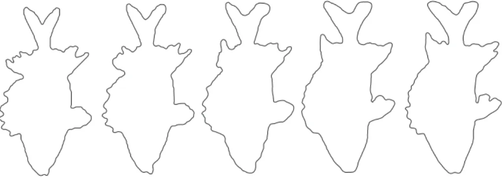
Fig. 4. Hausdorff warping a fish onto another.
We have borrowed the example in figure 4 from the database of fish sil-houettes (www.ee.surrey.ac.uk/Research/ VSSP/imagedb/demo.html) col-lected by the researchers of the University of Surrey at the center for Vision, Speech and Signal Processing (www.ee.surrey.ac.uk/Research/VSSP). This database contains 1100 silhouettes. A few steps of the result of Hausdorff warping one of these silhouettes onto another are shown in figure 4.
Figures 5 and 6 give a better understanding of the behavior of Hausdorff warping. A slightly displaced detail “warps back” to its original place (figure 5). Displaced further, the same detail is considered as another one and dis-appears during the warping process while the original one redis-appears (figure 6).
Fig. 5. Hausdorff warping boxes (i). A translation-like behaviour.
Fig. 6. Hausdorff warping boxes (ii). A different behaviour: a detail disappears while another one appears.
Finally, figures 7 and 8 show the Hausdorff warping between two open curves and between two closed surfaces, respectively.
Note also that other warpings are given by the minimization of other approximations of the Hausdorff distance. Figure 9 shows the warping of a rough curve to the silhouette of a fish and bubbles given by the minimization of the W1,2norm as explained in section 5.6. Our “level sets” implementation can deal with the splitting of the source curve while warping onto the target one. Mainly, when we have to implement the motion of a curve Γ under a velocity field v: Γt = v, we use the Level Set Method introduced by Osher and Sethian in 1987 [30, 34, 29].
Fig. 7.Hausdorff warping an open curve to another one.
Fig. 8. Hausdorff warping a closed surface to another one.
7 Application to the computation of the empirical mean
and covariance of a set of shape examples
We have now developed the tools for defining several concepts relevant to a theory of stochastic shapes as well as providing the means for their effective computation. They are based on the use of the function E defined by (25). 7.1 Empirical mean
The first one is that of the mean of a set of shapes. Inspired by the work of Fr´echet [13, 14], Karcher [20], Kendall [23], and Pennec [31], we provide the following (classical)
Definition 20. Given Γ1,· · · , ΓN, N shapes, we define their empirical mean as any shape ˆΓ that achieves a local minimimum of the function µ :S → R+ defined by Γ → µ(Γ, Γ1,· · · , ΓN) = 1 N X i=1,··· ,N E2(Γ, Γi)
Note that there may exist several means. We know from proposition 19 that there exists at least one. An algorithm for computing approximations to an empirical mean of N shapes readily follows from the previous section: start from an initial shape Γ0and solve the PDE
Γt=−∇µ(Γ, Γ1,· · · , ΓN) n (26)
Γ (0, .) = Γ0(.)
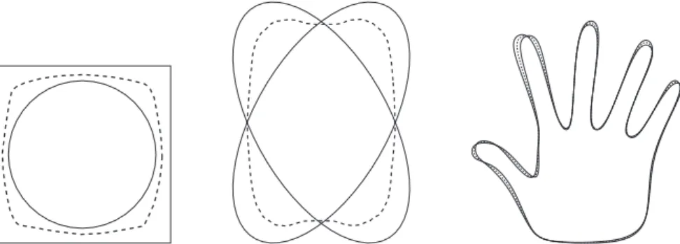
We show some examples of means computed by this algorithm in figure 10.
Fig. 10. Examples of means of several curves: a square and a circle (left), two ellipses (middle), and two hands (right).
When the number of shapes grows larger, the question of the local minima of µ may become a problem and the choice of Γ0 in (26) an important issue.
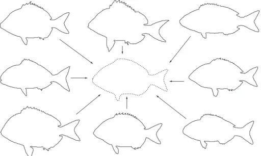
An example of mean is obtained from the previous fish silhouettes database: we have used eight silhouettes, normalized them so that their centers of grav-ity and principle axes were aligned, and computed their mean, as shown in figure 11. The initial curve, Γ0 was chosen to be an enclosing circle.
Fig. 11.The mean of eight fishes.
7.2 Empirical covariance
We can go beyond the definition of the mean and in effect define something similar to the covariance matrix of a set of N shapes.
The functionS → R+ defined by Γ → E2(Γ, Γ
i) has a gradient which defines a normal velocity field, noted βi, defined on Γ , such that if we con-sider the infinitesimal deformation Γ − βindτ of Γ , it decreases the value of E2(Γ, Γ
i). Each such βi belongs to L2(Γ ), the set of square integrable real functions defined on Γ . Each Γi defines such a normal velocity field βi. We consider the mean velocity ˆβ = 1
N PN
i=1βi and define the linear operator Λ : L2(Γ )
→ L2(Γ ) such that β →P
i=1,N < β, βi− ˆβ > (βi− ˆβ). We have the following
Definition 21. Given N shapes of S, the covariance operator of these N shapes relative to any shape Γ ofS is the linear operator of L2(Γ ) defined by
Λ(β) = X i=1,N
where the βi are defined as above, relatively to the shape Γ .
This operator has some interesting properties which we study next. Proposition 22. The operator Λ is a continuous mapping of L2(Γ ) into L2(Γ ).
Proof. We havekP
i=1,N < β, βi− ˆβ > (βi− ˆβ)k2≤Pi=1,N| < β, βi− ˆβ > |kβi− ˆβk2and, because of Schwarz inequality,| < β, βi− ˆβ >| ≤ kβk2kβi− ˆβk2. This implies that kP
i=1,N < β, βi− ˆβ > (βi − ˆβ)k2 ≤ Kkβk2 with K = P
i=1,Nkβi− ˆβk22.
Λ is in effect a mapping from L2(Γ ) into its Hilbert subspace A(Γ ) gener-ated by the N functions βi− ˆβ. Note that if Γ is one of the empirical means of the shapes Γi, by definition we have ˆβ = 0.
This operator acts on what can be thought of as the tangent space to the manifold of all shapes at the point Γ . We then have the
Proposition 23. The covariance operator is symmetric positive definite. Proof. This follows from the fact that < Λ(β), β >=< β, Λ(β) >=P
i=1,N < β, βi− ˆβ >2.
It is also instructive to look at the eigenvalues and eigenvectors of Λ. For this purpose we introduce the N× N matrix ˆΛ defined by ˆΛij =< βi− ˆβ, βj−
ˆ
β >. We have the
Proposition 24. The N× N matrix ˆΛ is symmetric semi positive definite. Let p ≤ N be its rank, σ2
1 ≥ σ22 ≥ · · · ≥ σp2 > 0 its positive eigenvalues, u1,· · · , uN the corresponding eigenvectors. They satisfy
ui· uj = δij i, j = 1,· · · , N ˆ
Λui= σi2ui i = 1,· · · , p ˆ
Λui= 0 p + 1≤ i ≤ N
Proof. The matrix ˆΛ is clearly symmetric. Let now α = [α1,· · · , αN]T be a vector of RN, αTΛα =ˆ
kβk2
2, where β =P N
i=1αi(βi− ˆβ). The remaining of the proposition is simply a statement of the existence of an orthonormal basis of eigenvectors for a symmetric matrix of RN.
The N -dimensional vectors uj, j = 1,· · · , p and the p eigenvalues σ2k, k = 1,· · · , p define p modes of variation of the shape Γ . These modes of variation are normal deformation flows which are defined as follows. We note uij, i, j = 1,· · · , N the ith coordinate of the vector uj and vj the element of A(Γ ) defined by
(27) vj = 1 σj N X i=1 uij(βi− ˆβ)
In the case Γ = ˆΓ , ˆβ = 0. We have the proposition
Proposition 25. The functions vj, j = 1,· · · , p are an orthonormal set of eigenvectors of the operator Λ and form a basis of A(Γ ).
The velocities vk, k = 1,· · · , p can be interpreted as modes of variation of the shape and the σ2
k’s as variances for these modes. Looking at how the mean shape varies with respect to the kth mode is equivalent to solving the following PDEs:
(28) Γt=±vkn
with initial conditions Γ (0, .) = ˆΓ (.). Note that vk is a function of Γ through Λ which has to be reevaluated at each time t. One usually solves these PDEs until the distance to ˆΓ becomes equal to σk.
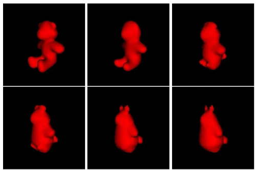
An example of this evolution for the case of the fingers is shown in figure 12. Another interesting case, drawn from the example of the eight fish of figure 11, is shown in figure 13 where the first four principal modes of the covariance operator corresponding to those eight sample shapes are displayed.
8 Further comparison with other approaches and
conclusion
We have presented in section 1 the similarities and dissimilarities of our work with that of others. We would like to add to this presentation the fact that ours is an attempt to generalize to a nonlinear setting the work that has been done in a linear one by such scientists as Cootes, Taylor and their collabora-tors [5] and by Leventon et al. who, like us, proposed to use distance functions to represent shapes in a statistical framework but used a first-order approxi-mation by assuming that the set of distance functions was a linear manifold [26, 25] which of course it is not. Our work shows that dropping the incorrect linearity assumption is possible at reasonable costs, both theoretical and com-putational. Comparison of results obtained in the two frameworks is a matter of future work.
In this respect we would also like to emphasize that in our framework the process of linear averaging shape representations has been more or less replaced by the linear averaging of the normal deformation fields which are tangent vectors to the manifold of all shapes (see the definition of the covari-ance operator in section 7.2) and by solving a PDE based on these normal deformation fields (see the definition of a mean in section 7.1 and of the de-formation modes in section 7.2).
Fig. 12. The first three modes of variation for nine sample shapes and their mean. The mean is shown in thick continuous line, the solutions of equation (28) for k = 1, 2, 3 are represented in dotted lines.
It is also interesting to recall the fact that our approach can be seen as the opposite of that consisting in first building a Riemannian structure on the set of shapes, i.e. going from an infinitesimal metric structure to a global one. The infinitesimal structure is defined by an inner product in the tangent space (the set of normal deformation fields) and has to vary continuously from point to point, i.e. from shape to shape. As mentioned before, this is mostly dealt with in the work of Miller, Trouv´e and Younes [28, 40, 45]. The problem with these approaches, beside that of having to deal with parametrizations of the shapes, is that there exist global metric structures on the set of shapes (see
Fig. 13. The first four modes of variation for the eight sample shapes and their mean shown in figure 11. The mean is shown in thick continuous line, the solutions of equation (28) for k = 1, · · · , 4 are represented in dotted lines.
section 2.2) which are useful and relevant to the problem of the comparison of shapes but that do not arise from an infinitesimal structure.
Our approach can be seen as taking the problem from exactly the opposite viewpoint from the previous one: we start with a global metric on the set of shapes (ρH or the W1,2 metric) and build smooth functions (in effect smooth approximations of these metrics) that we use as dissimilarity measure or en-ergy functions and minimize using techniques of the calculus of variation by computing their gradient and performing infinitesimal gradient descent. We have seen that in order to compute the gradients we need to define an inner-product of normal deformation flowss and the choice of this inner-inner-product may influence the way our algorithms evolve from one shape to another. This last point is related to but different from the choice of the Riemaniann metric in the first approach. Its investigation is also a topic of future work.
Another advantage of our viewpoint is that it apparently extends gra-ciously to higher dimensions thanks to the fact that we do not rely on parametrizations of the shapes and work intrinsically with their distance func-tions (or approximafunc-tions thereof). This is clearly also worth pursuing in future work.
References
1. Bookstein FL (1986) Size and shape spaces for landmark data in two dimensions. Statistical Science 1:181–242
2. Carne TK (1990) The geometry of shape spaces. Proc. of the London Math. Soc. 3(61):407–432
3. Charpiat G, Faugeras O, Keriven R (2004) Approximations of shape metrics and application to shape warping and empirical shape statistics. Foundations of Computational Mathematics
4. Choquet G (1969) Cours d’Analyse, volume II. Masson
5. Cootes T, Taylor C, Cooper D, Graham J (1995) Active shape models-their training and application. Computer Vision and Image Understanding 61(1):38– 59
6. Delfour MC, Zol´esio J-P (July 1994) Shape analysis via oriented distance func-tions. Journal of Functional Analysis 123(1):129–201
7. Delfour MC, Zol´esio J-P (1998) Shape analysis via distance functions: Local theory. In: Boundaries, interfaces and transitions, volume 13 of CRM Proc. Lecture Notes, pages 91–123. AMS, Providence, RI
8. Delfour MC, Zol´esio J-P (2001) Shapes and geometries. Advances in Design and Control. Siam
9. Dryden IL, Mardia KV (1998) Statistical Shape Analysis. John Wiley & Son
10. Dupuis P, Grenander U, Miller M (1998) Variational problems on flows of dif-feomorphisms for image matching. Quarterly of Applied Math. 56:587–600
11. Evans LC (1998) Partial Differential Equations, volume 19 of Graduate Studies in Mathematics. Proceedings of the American Mathematical Society
12. Federer H (1951) Hausdorff measure and Lebesgue area. Proc. Nat. Acad. Sci. USA 37:90–94
13. Fr´echet M (1944) L’int´egrale abstraite d’une fonction abstraite d’une variable abstraite et son application `a la moyenne d’un ´el´ement al´eatoire de nature quel-conque. Revue Scientifique, pages 483–512 (82`eme ann´ee)
14. Fr´echet M (1948) Les ´el´ements al´eatoires de nature quelconque dans un espace distanci´e. Ann. Inst. H. Poincar´e X(IV):215–310
15. Fr´echet M (1961) Les courbes al´eatoires. Bull. Inst. Internat. Statist. 38:499–504
16. Grenander U (1993) General Pattern Theory. Oxford University Press
17. Grenander U, Chow Y, Keenan D (1990) HANDS: A Pattern Theoretic Study of Biological Shapes. Springer-Verlag
18. Grenander U, Miller M (1998) Computational anatomy: an emerging discipline. Quart. Appl. Math. 56(4):617–694
19. Harding EG, Kendall DG, editors (1973) Stochastic Geometry, chapter Foun-dation of a theory of random sets, pages 322–376. John Wiley Sons, New-York
20. Karcher H (1977) Riemannian centre of mass and mollifier smoothing. Comm. Pure Appl. Math 30:509–541
21. Kendall DG (1984) Shape manifolds, procrustean metrics and complex projec-tive spaces. Bulletin of London Mathematical Society 16:81–121
22. Kendall DG (1989) A survey of the statistical theory of shape. Statist. Sci. 4(2):87–120
23. Kendall W (1990) Probability, convexity, and harmonic maps with small image i: uniqueness and fine existence. Proc. London Math. Soc. 61(2):371–406
24. Klassen E, Srivastava A, Mio W, Joshi SH (2004) Analysis of planar shapes using geodesic paths on shape spaces. IEEE Transactions on Pattern Analysis and Machine Intelligence 26(3):372–383
25. Leventon M, Grimson E, Faugeras O (June 2000) Statistical Shape Influence in Geodesic Active Contours. In: Proceedings of the International Conference on Computer Vision and Pattern Recognition, pages 316–323, Hilton Head Island, South Carolina. IEEE Computer Society
26. Leventon M (2000) Anatomical Shape Models for Medical Image Analysis. PhD thesis, MIT
27. Matheron G (1975) Random Sets and Integral Geometry. John Wiley & Sons
28. Miller M, L. Younes (2001) Group actions, homeomorphisms, and matching: A general framework. International Journal of Computer Vision 41(1/2):61–84
29. Osher S, Paragios N, editors (2003) Geometric Level Set Methods in Imaging, Vision and Graphics. Springer-Verlag
30. Osher S, Sethian JA (1988) Fronts propagating with curvature-dependent speed: Algorithms based on Hamilton–Jacobi formulations. Journal of Computational Physics 79(1):12–49
31. Pennec X (December 1996) L’Incertitude dans les Probl`emes de Reconnaissance et de Recalage – Applications en Imagerie M´edicale et Biologie Mol´eculaire. PhD thesis, Ecole Polytechnique, Palaiseau (France)
32. Rudin W (1966) Real and Complex Analysis. McGraw-Hill
33. Serra J (1982) Image Analysis and Mathematical Morphology. Academic Press, London
34. Sethian JA (1999) Level Set Methods and Fast Marching Methods: Evolv-ing Interfaces in Computational Geometry, Fluid Mechanics, Computer Vision, and Materials Sciences. Cambridge Monograph on Applied and Computational Mathematics. Cambridge University Press
36. Soatto S, Yezzi AJ (May 2002) DEFORMOTION, deforming motion, shape average and the joint registration and segmentation of images. In: Heyden A, Sparr G, Nielsen M, Johansen P, editors, Proceedings of the 7th European Con-ference on Computer Vision, pages 32–47, Copenhagen, Denmark. Springer– Verlag
37. Sussman M, Smereka P, Osher S (1994) A Level Set Approach for Comput-ing Solutions to Incompressible Two-Phase Flow. J. Computational Physics 114:146–159
38. Toga A, Thompson P (2001) The role of image registration in brain mapping. Image and Vision Computing 19(1-2):3–24
39. Toga A, editor (1998) Brain Warping. Academic Press
40. Trouv´e A (1998) Diffeomorphisms groups and pattern matching in image anal-ysis. The International Journal of Computer Vision 28(3):213–21
41. Trouv´e A, Younes L (June 2000) Diffeomorphic matching problems in one di-mension: designing and minimizing matching functionals. In: Proceedings of the 6th European Conference on Computer Vision, pages 573–587, Dublin, Ireland
42. Trouv´e A, Younes L (February 2000) Mise en correspondance par
diff´eomorphismes en une dimension: d´efinition et maximisation de fonction-nelles. In: 12`eme Congr`es RFIA‘00, Paris
43. Younes L (1998) Computable elastic distances between shapes. SIAM Journal of Applied Mathematics 58(2):565–586
44. Younes L (1999) Optimal matching between shapes via elastic deformations. Image and Vision Computing 17(5/6):381–389
45. Younes L (2003) Invariance, d´eformations et reconnaissance de formes. Math´ematiques et Applications. Springer-Verlag