Published in Computer Methods in Biomechanics and Biomedical Engineering, 2011, doi: 10.1080/10255842.2011.613379 Link to publication: http://www.tandfonline.com/doi/abs/10.1080/10255842.2011.613379
Detection of incoherent joint state due to inaccurate bone motion
estimation
Cédric SCHWARTZ (1,2,5), Fabien LEBOEUF (4), Olivier RÉMY-NÉRIS (1,3,5), Sylvain
BROCHARD (1,3), Mathieu LEMPEREUR (1,3), Valérie BURDIN (1,2,5)
1 - LaTIM, Inserm U650, Brest, France 2 - Telecom Bretagne, Institut Telecom, Brest, France
3 - Service de médecine physique et de réadaptation, CHU Brest, Brest, France 4 - Pôle médecine physique et réadaptation, CHU Nantes, Nantes, France
5 - Université Européenne de Bretagne, Rennes, France
In biomechanical modeling and motion analysis, the use of personalized data such as bone geometry would provide more accurate and reliable results. However, there is still a limited number of tools used to measure the evolution of articular interactions. This paper proposes a coherence index to describe the articular status of contact surfaces during motion. The index relies on a robust estimation of the evolution of surfacic interactions between the joint surfaces. The index is first compared to distance maps on simulated motions. It is then used to compare two motion capture protocols (two different localizations of the markers for scapula tracking). The results show that the index detects progressive modifications in the joint and allows to distinguish the two protocols, in accordance with the literature. In the future, the index could, among other things, be used to compare / improve biomechanical models and motion analysis protocols.
Keywords: joint; coherence; glenohumeral joint; motion analysis; musculoskeletal model; soft tissue artifacts
Introduction
Joints play a major role in human skeleton architecture as they allow bone mobility and functionality. An accurate description of the motion of joint components is one of the key features for accurate diagnosis of articular pathologies or the design of biomechanical models for medical ends (Hill et al. 2008). Joints are complex structures, whose stabilization includes both active and passive elements. Subject-specific anatomy is rarely taken into account in biomechanical modeling and motion analysis.
Musculo-skeletal models of the whole body have reached a level of sophistication that has made them a common tool for biomechanical research (Damsgaard et al. 2006, Delp et al. 2007). However, one essential aspect that is still missing before these models can be used in a clinical setting is the ability to analyze specific patients. Usually, a ”standard” model (Klein Horsman et al., 2007) is scaled to be adapted to the studied subject. The most common scaled parameters are weight and segment lengths (Rasmussen et al., 2005). This approach leads to a model, which is still relatively general, and which only takes into account limited physiological and anatomical specificities of the subject. Lee (Lee et al., 2010) has however shown that an anatomically based
knee joint offers a more accurate description of the kinematic and dynamic than a purely geometrical joint. Therefore anatomical information has the potential to be used to create better subject-specific models.
Medical imaging systems like MRI (Graichen et al., 2000) or bone pin clusters (Karduna, 2001) allow accurate 3D estimation of bone positions. However, these methods are either static or invasive. Consequently, opto-electronic markers and magnetic sensors are the most commonly used motion capture systems. Their main advantage is the possibility of acquiring movements under wide range of dynamic conditions. Unfortunately, the measurements are not directly linked to bone movement but to skin deformation and thus lead to a lack of accuracy in the estimation of bone position. Several methods were proposed in the literature to correct soft tissue artifacts. Some of them use anatomical knowledge, such as global optimization (Lu et al., 1999), which fixed the number of degrees of freedom according to an anatomical description of the joint. However, using simple mechanical joints has been shown not to improve motion estimation (Andersen, 2009). Introducing anatomical data for better joint description would therefore result in improvements in biomechanical modeling. Unfortunately few tools are available to make use of this information.
Joint functionality analysis is based on the study of bone relationships. The local geometry of the joint can be estimated by measuring Euclidean distances between anatomical landmarks and/or by determining the location of contact points between bones (Freeman et al. 2005; Wolf et al. 2008). The main limitation of these approaches lies in the geometric complexity of the bone surfaces, which is not taken into account when focusing on a limited number of points. The congruence of a joint can be defined as the morphological adequacy of one articular surface to another (Hamilton 1996; Kralovic 2000). Such analysis leads to a surfacic approach. McLaughlin (McLaughlin et al. 2005) and Kralovic (Kralovic 2000) used a root mean square congruence index (Ateshian et al. 1992) based on the comparison of the main curvatures on each facing articular surface. Some authors completed this analysis by proposing distance maps, which give the nearest region on the opposite bone (Anderst et al. 2003; Windisch et al. 2007). The distance maps are a simple but powerful tool to detect abnormal situations. However, the relevance of these measures is directly linked to the accuracy of the surface description (acquisition resolution, visible structures such as bone, cartilage, menisci) issued from the segmentation process and their positioning in space. Thus, the performance of the acquisition system and
of the post-processing procedures (segmentation, meshing) strongly influences on the based distance maps methods. Unfortunately, not all systems are able to provide sufficient accuracy. Thus, even in the healthy joint, incoherent states (such as dislocation) may occur because the acquisition system is unable to give the true functionality.
Few studies tried to measure the appearance of bone positioning errors. Defining collisions remains a challenge and only measures for specific situations, such as the rotation of the hip (Arbabi et al. 2009), exist. Thus, an index dedicated to inform about the appearance of errors in bone positioning would add information to existing tools.
The goal of this paper is to propose an index, which measures the articular state in joints. Such an index aims to provide a new tool for personalized biomechanics using joint anatomy. After the mathematical description of the index, simulated motions demonstrate how the index works and its differences of behavior compared to distance maps. An example of how to use the index in a real-case scenario is also presented (comparison of several protocols of shoulder 3D motion analysis). It also includes the registration procedure of the bones, which was acquired separately.
Materials and methods
Mathematical description of the joint coherence index
The computation of the joint coherence index relies on two main steps. First, the relative position of the articular surfaces is evaluated (matching process). This position is then compared to a reference position (evaluation process).
Matching process
The bone surface can be represented in different ways including symbolic representations and meshes. In this paper, we assume that surfaces are described using triangular meshes. To evaluate the relative position of the surfaces, facing vertices of the two articular surfaces are matched. Soslowsky (Soslowsky et al. 1992) proposed to find the nearest point of each vertex in the outward-pointing normal direction to the surface within a specified range. In our situation, because of potential bone placement errors, articular surfaces may not be in contact. The search range for the nearest point in the normal direction (10 meters in our implementation) should therefore be superior to the maximal expected dislocation distance. Finding the nearest point in the opposite direction of the normal vector indicates that the two surfaces are overlapping. In situations, such as biomechanical modeling, users usually want to prevent collision
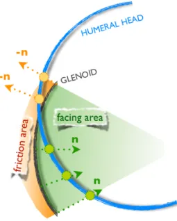
between bones. However because of unavoidable biases in the 3D reconstruction of the bone (imaging system limitations, image segmentation and processing errors), small depth collisions may occur. Therefore, if no point is found in the normal direction, the search is performed in the opposite direction, but limited to a region (Fig. 1), called the friction region. The user defines the depth of the friction region in accordance to the desired behaviour of the index. In order to label points lying in the friction region, distances to these points are set negative. Matched vertices, whose scalar product between normal vectors to their respective surfaces is superior to 0, are not taken into account. In other words, it consists in rejecting non-facing local areas. Besides, the measurement of distances between the facing vertices makes it possible to establish distance maps and to compute the contact area (CA) by summing the area of all triangles lying within a search range [-5 mm; +10 mm] around the glenoid surface.
Figure 1 - Description of the process of matching between the vertices of the glenoid (grey curve) and of the humeral head (blue curve). The facing vertices (green circles) of the glenoid are searched at first is their normal vector directions (green arrows). If no vertex is found, the facing vertices (orange circles) are searched in the opposite direction (orange arrow) within a certain distance (orange area).
Evaluation process
The state of the joint depends on the relative position of the two articular surfaces. From the matching process described in the previous section, we define, at each time t of the motion, the number N(t) of facing vertices and the average distance D(t) between them.
To quantify the instantaneous state of the joint, the index can refer to a position known as physiological. The mesh representation of the bones coming from 3D anatomical imaging can usually be used as a reference for joint coherence (N(0), D(0)).
Indeed few clinical situations, such as joint luxation, do not allow such use. The articular state is then evaluated as the variation between the reference and the studied situations. Residues of the number of facing vertices (N(0)-N(t)) and of the average distance between the facing vertices (D(0)-D(t)) are computed for each instant of the motion. Through the use of an estimator, the residues can be normalized as weights ranging from 0 to 1. A weight close to 1 reflects small difference from the reference.
One Tukey M- estimator is used for each term of the index: the Facing Vertices term FV(t) (Eq. (1)) and the Average Distance term AD(t) (Eq. (2)).
(1)
(2)
where rN and rD are respectively the reject points of the estimators for the facing vertices term (FV) and the average distance term (AD).
The choice of the reject point values has an important influence on the behavior of the index. Smaller values for the reject point will increase its ability to distinguish two different behaviors, whereas larger values increase its ability to identify two
similar behaviors. Therefore, the values should be adapted to i/ the goal of the study, ii/ the anatomical characteristics of the studied joint. An example of choice is presented in the “Simulated motions study” section.
When facing vertices are found in the friction region, the distance between the matching points is marked as negative. Therefore, the positioning of vertices in the friction region influences the average distance term. The magnitude of this influence is directly linked to the number of vertices lying in the friction region as well as the amplitude of penetration depth.
The expression of the articular coherence index ACI(t) is finally the product of AD(t) and FV(t) as presented in Eq. (3).
(3)
Simulated motions study
MRI anatomical acquisitions of the scapula and the humerus were performed. After segmentation, scapula and humerus meshes were reconstructed. A quadric robust-fitting approach (Allaire et al. 2007) was used to model the humeral head. This fitting method resulted in an ellipsoidal (nearly spherical) shape and enables the determination of the intrinsic
features of the joint: the location of the anatomical center of the head as well as the major axes of the shape. Detailed description of all this procedure can be found in Lempereur et al., 2010. For the purpose of the simulation, the glenoid surface was considered as fixed.
In order to study the behavior of the distance maps and the proposed index several simulations where carried out. The first simulated motion aims to simulate a situation, which may occur in a bio-inspired mechanical model whereas the two others focus on errors, which may occur during a motion estimated thanks to a marker-based system. Such a system can induce relatively important errors. Therefore we chose to apply an extra-simulated displacement in two directions. The following three simulated movements of the glenohumeral joint were carried out:
• Model-based elevation of the arm: one common gleno-humeral joint model is the ball and socket joint (Yan et al., 2010). The center of rotation is estimated as the anatomical center of the humeral head (Veeger 2000). The simulated motion is a rotation of the humerus around the major symmetry axis of the fitted ellipsoid (abduction-like axis). A rotation of 60 degrees was applied. • Decreasing the distance between the joint
approximated abduction axis was applied plus a translation of 20 mm in the opposite direction of the mean normal vector of the glenoid surface. • Increasing the distance between the joint surfaces:
the same 60° rotation around the approximated abduction axis was applied plus a translation of 20 mm in the direction of the mean normal vector of the glenoid surface.
As emphasized in the “Mathematical description of the joint coherence index” section, the choice of the reject points of the index should be adapted to the study. Here the objective is to evaluate the evolution of the joint state in several motions. If the index is too sensitive, it will produce false positives for all motions. On the other hand, if the index is too specific, it will produce false negatives. In both cases, the index will not be able to correctly evaluate the state of the joint during the motions. For this study, rD = 15 mm and rN = N(0) was found to be a good compromise. Anatomically speaking, 15 mm is approximately 1/3 of the mean diameter of the humeral head (Boileau et al. 1997) and choosing rN =
N(0) implies that when no facing vertice is found, the
index is equal to zero. The friction zone was equal to 5 mm. This value is small to emphasize the influence of collision on the result of the index.
In-vivo study
This index is tested on experimental motions with the objective of comparing two motion analysis protocols for shoulder movement estimation. Data have been collected on a healthy volunteer (age: 25, weight: 83 kg, height: 1.85 m). Measurements were carried out on the right arm. The volunteer had no history of pain, trauma or surgery and the protocol was ratified by the local ethics committee. The subject lay initially in a prone position with the humerus along the trunk and then did a maximal humerus elevation in the sagittal plane.
The scapula and humerus motion were measured using an opto-electronic tracking device (VICON, Oxford Metrics Limited, Oxford). 120 markers were placed over the scapula in order to cover the bone completely and to ensure the best registration of the bones in the kinematic coordinate system (see infra). From all markers, two cluster shapes were differentiated. The first one included all available markers on the scapula: the whole cluster (WClust), whereas the second one was only composed of the 31 markers lying on the acromion and the upper side of the posterior face of the scapula: the acromion cluster (AClust). The estimation of the scapula motion was then carried out on the two clusters using the IMCP algorithm (Jacq et al. 2008),
which is a robust, simultaneous and multi-object extension of the classic algorithm of registration ICP (Iterative Closest Point) (Besl et al. 1992). In this way we were able to compare the changes of the index in two different conditions. An additional cluster of 16 technical markers was placed on the middle of the arm segment to define humerus position. An extra marker placed on the lateral epicondyle was also used. The estimation of the motion of the humerus was carried out with the least-square method detailed in (Söderkvist et al., 1993).
The visualization of the markers in the MRI was used to perform the registration of both scapula and humerus in the kinematic coordinate system given by the Vicon system. This procedure assumes that the relative position of the markers clusters and the bone are similar during the MRI and motion capture acquisitions. Consequently, the glenohumeral joint was imaged with the volunteer lying in a similar position as during the motion acquisition: prone position with the humerus along the trunk. As the motion analysis markers are not visible in any MRI sequence, 5 mm spherical candies (Hollywood Bulles Oxygen ®) were placed at the same position as the motion marker. In order to avoid errors during markers replacement, their positions were marked on the skin before positioning the markers on the skin.
Additional information about the registration procedure can be found in Lempereur et al., 2010 or in Schwartz, 2009.
The index parameters were identical to those in the simulated motions study. Indeed, these values allow good comparison between a wide range of motions, which is the case here when comparing two acquisition protocols. The values of the reject points are quite large because we are not measuring small variations induced by a pathology but rather large errors due to soft tissue artifacts. The value of the friction zone would have probably been too small if the estimated motions had led to important collision, which was not the case in this example.
Results
Simulated motions study
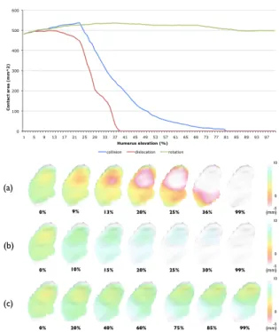
The evolution of the articular coherence index (ACi), as well as both terms used for its computation (average distance term (AD) and facing vertices term (FV)), are presented for the three simulated motions (figures 2, 3, 4). The contact area (CA) is shown in figure 5.
Figure 2 – Articular coherence index (ACI) during the simulated rotation of the humerus around the humeral head and the 2 terms, which compose ACI: average distance term (AD) and facing vertices term (FV). The biomechanical model is applied on the real anatomical center of the humeral head
Figure 3 – Articular coherence index (ACI) during the simulated decreasing distance motion between articular surfaces (60° rotation and 20 mm translation) and the 2 terms, which compose ACI: average distance term (AD) and facing vertices term (FV).
Figure 4 – Articular coherence index (ACI) during the simulated increasing distance motion between articular surfaces (60° rotation and 20 mm translation) and the 2 terms, which compose ACI: average distance term (AD) and facing vertices term (FV).
Figure 5 – Evolution of the contact area on the glenoid. For glenoid surface distance maps, polygons are colored according to minimum distance from the opposing bone surface (humeral head surface): (a) during the simulated collision of the humerus, (b) during the simulated dislocation of the humerus, (c) during the simulated rotation of the humerus.
Figure 2 displays ACi, AD and FV curves of the simulated motion of the humerus constrained to rotate around the abduction axis. The curve of ACi shows a moderate decrease during the motion. Its value remains superior to 0.68. This decrease is directly linked to AD, which decreases in a similar way. FV remains approximately equal to 1 during the entire motion. CA, presented in figure 5, slightly increases during the first 37% of the movement from 481 mm2 to 536 mm2. During the rest of the
For the motion with decreasing distance between the faces of the joint, figure 3 shows a gradual decrease of ACi. ACi becomes lower than 0.1 as soon as 45% of the movement is completed. In the first quarter of the motion, the curves of ACi and AD are similar. Then AD becomes relatively stable and ranges from 0.27 to 0.48. FV remains near 1 during the first 30% of the motion and then quickly decreases to zero from the second third of the motion. CA (figure 5) increases during the first quarter of the motion from 481 mm2 to 537 mm2. Then it decreases to 7 mm2 when 70% of the movement has been
performed.
The motion with increasing distance between the faces of the joint leads to high gradient decrease of ACi (figure 4). ACi is lower than 0.1 as soon as 25% of the motion is performed. AD evolution is similar to that of ACi while FV is nearly equal to 1 during the entire motion. In figure 5, CA remains relatively stable during the first 20% of the motion. Then CA decreases very quickly to be equal to 0 mm2
as soon as 40% of the motion has been performed.
Experimental example study
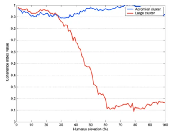
Figure 6 - Coherence index during real arm elevation motion. Scapula motion is estimated with IMCP algorithm on a cluster covering the whole scapula (WClust) or only the acromion and the upper anterior face of the scapula (AClust).
Figure 6 shows the evolution of the articular coherence index (ACI) when using WClust or AClust during the real humeral elevation. The coherence ACI of the subject remains between 0.9 and 1 during all the elevation of the arm with AClust. With WClust, the ACI starts to decrease from 30% of the motion and stabilizes between 0.1 and 0.2 during the last 40% of the arm elevation.
Discussion
A specific articular coherence index has been designed for situations where bone position is misestimated. The simulation study is used to show the pattern of this new index when the faces of the joint will not remain facing each other in comparison to classic distance maps. The applicability of the
index is then shown on an experimental motion. Because of the large influence of soft tissues artifacts for scapula, the glenohumeral joint was chosen for the experimental motion example.
Comparison of the distances maps and the coherence index on simulated motions
For accurate positioning of the bones, the analysis of the location of the contact area (Soslowsky et al. 1992; Kelkar et al. 2001) or the distance between bone landmarks in the joint provides information about normal or pathological behavior of the joint. The localization and quantification of the contact between the articular surfaces contribute to the understanding of the stress repartition and may reveal abnormal situations and pathologies (Koo et al., 2007). However, our simulations revealed that the contact area (CA) does not provide relevant information for inaccurate bone positioning. During the simulated movement of rotation around the humeral head center, the humeral head stays in front of and near the glenoid. CA, which measures the whole surface of the humeral head staying within a specific range of the glenoid, does not evolve significantly during the motion (maximum variation of 11.4%). At the end of the motion, the difference of contact area from the initial position is only equal to 3.5%. This small variation does not reflect the fact
that the inferior part of the humeral head has progressively moved away from the glenoid as can be observed on the distance maps of the glenoid (Fig. 5 (c)). The dislocation of the joint is simulated by a translation of the humerus in the same direction of the mean normal vector of the glenoid. Consequently, the humeral head stays opposite to the glenoid. As long as the humeral head remains in the range defined as contributing to the surface contact measurement, CA is stable. Then, the fall of CA is very sharp. The distance maps show the disappearance of the contact between 20 and 30% of progress instants of the motion. CA is measured by integrating the mesh surface within a specific range. Therefore, a vertex is classified in a binary way as in contact or not in contact with the opposite articular surface. Anderst (Anderst et al. 2003) proposed to study separately sub-ranges of the complete region participating in the contact area. However, this approach leads to numerous curves (one for each sub-range) and therefore a more difficult analysis of the results. The main reason for the poor performance of the CA analysis in our simulation is that CA computation relies on the hypothesis of actual contact between the articular surfaces, which is clearly not always the case. Adding a term, which takes into account the distance between the surfaces, is one of the contributions of our index.
The proposed index has been designed to allow progressive quantification of the evolution of the relation between the two facing articular surfaces. The simulated collision forces the humerus to progressively get closer to the scapula. The first part of the motion did not induce bone collision, which only appears at 20% of the total displacement. This is related to our MRI sequence that did not allow defining with precision the thickness of the cartilage. Indeed we had to reach a compromise between the visualization of markers (the candies) and the definition of the bone shape. After this limit, AD decreased and ACI too. Secondly, with the effective collision of the bones the number of facing vertices decreased. It causes AD to decrease too and consequently ACI continues to decrease with the augmentation of the inter-penetration depth. Contrary to CA, ACI measured the variation of the articular coherence until a non physiological relative position of humerus and scapula. During dislocation, the distance between the humeral head and the glenoid gradually increased and AD and ACI decreased. The index measured the continuous variation of the joint coherence. The index can also measure small coherence variations as during the movement of rotation around the humeral head center. Indeed, ACI decreased with the increase of the average distance between the two articular surfaces.
The three simulated motions illustrated situations where incoherent states occur. These situations may happen when the motion is estimated with external markers or when using biomechanical models. The simulations reveal some limitations of the distance maps to study the articular coherence. On the contrary, the proposed index seems to be able to distinguish situations linked to an inaccurate positioning of the bones.
Measuring protocol quality with the coherence index on in-vivo motions
The results obtained in our subject show that the position of the marker cluster has a great influence on joint coherence. The AClust contributes to better coherence in the joint. During the first 30 degrees of elevation, the ACI is quite similar to both AClust and
WClust. However after 60° the ACI is low (between
0.1 and 0.2) with WClust whereas the AClust remains superior to 0.9, which means better glenohumeral coherence. Soft tissue artifacts include muscle deformations, the inertial effects of the soft tissues motion as well as the relative motion of the skin and the bones. These artifacts are the largest source of error when the motion is estimated with makers placed on the skin (Leardini et al., 2005). The acromion region has been shown to be less influenced by soft tissue artifacts. Matsui (Matsui et al. 2006),
measured the deviation of skin marker from bone target equal to 40 to 50 mm on the acromion against 85 mm for the inferior angle of the scapula. Reduced relative motion of the underlying bone and the skin may explain the better results. Indeed Cappozzo (Cappozzo et al. 1995) recommended placing the markers where relative motion is minimal. Moreover, the acromion region is often chosen when using an electromagnetic device for motion analysis (Meskers et al. 2007). Karduna (Karduna et al., 2001) showed with pins drilled in the scapula that before 120° of arm elevation the use of a magnetic tracking device on the acromion offered reasonably accurate estimation of the motion. Even if the use of intra-cutaneous pins may modify the skin deformation by fixing the skin, Karduna (Karduna et al., 2001) study tends to confirm the interest of placing markers on the acromion. Van Andel (Van Andel et al. 2009) also pointed out the acromion region. His study leads to a small difference (6°) in humerus forward flexion and abduction between a palpation method and the kinematic provided by a cluster of three markers fixed on the acromion.
In this example, we show how the proposed index could be used to compare acquisition protocols and their ability to provide correct estimation of bone motion. Results obtained are in agreement with the
literature and thus emphasizes the interest of the index for non-invasive and dynamic evaluation of motion capture protocols. Of course, the use of the proposed index should not be limited to the study of motion analysis protocols but should also be extended, for example, to the comparison of joint biomechanical models. Preliminary results on this theme have already been presented by Leboucher (Leboucher et al. 2009) using the proposed index. The elbow is usually modeled as a revolute joint. Leboucher compared the impact of different axis choices on the coherence of the joint during flexion. He showed that an axis estimated through quadric fitting of the articular surfaces significantly improved the model compared to an axis running through the 2 epicondyles. It should also be noted that this index measure variations of the articular state but don’t give information about the origins of these variations (motion measurement errors, modeling inaccuracies, functional pathologies such as misbalance in ligament tension).
Practical use of the proposed index
The results of the coherence index are dependent on the registration between both anatomical and kinematic data, which can be relatively complex. In the experimental example presented in this paper, the fusion process implies the registration of the
anatomical data with the kinematic ones, thanks to the localization of the marker clusters in the initial position. The use of skin markers makes the procedure more difficult because of possible shifts between the bones and the skin surface. Indeed, as the registration is based on the scapula marker cluster, it requires that no relative motion between the markers and the bone occurs between the two acquisitions. This condition is difficult to perform in a very mobile joint such as the glenohumeral one, where soft tissue artifacts are significant. Therefore, subjects were placed in similar initial positions for both anatomical and kinematic acquisitions. This limitation is, of course, far less sensitive for joints where the relative skin shift is smaller as in the elbow or knee joint.
Errors during reconstruction of the articular surfaces are related to the choice of the imaging technique, the image resolution, and the chosen sequence. In this study the chosen MRI sequence does not allow accurate cartilage segmentation and therefore limits the definition of the joint surfaces. The quality of the mesh can also have an influence, when studying small variations in the joint. However, in the presented study, the errors created by the soft tissue artifacts were largely dominant. In order to limit the influence of small bias on the final coherence analysis, the coherence index needs to use
a robust weight function. Statistic theories introduce several robust estimators (Rousseeuw et al. 1987). The influence function of an estimator characterizes the bias introduced by a particular measure on the final solution. For robust estimator, the influence function should not indefinitely grow when measures increase. Huber (Huber, 1981) and Tukey M- estimators influence functions saturate for large values. However only the Tukey M- estimator suppresses completely aberrant data and was consequently retained. Aberrant data correspond to relative positions of the bones, which are significantly different from the reference position. Therfore, the choice of a Tukey weigh-estimator allows a far more robust index than if a simple binary operator based on a threshold value had been used. Moreover, variations of the contact area occur during a physiological movement (Soslowsky et al. 1992). The index should also be robust to these normal variations compared to the reference position extracted from the anatomical acquisition.
The choice of the index parameters and in particular the values of the reject points rD and rN is a key aspect when using the proposed index. As previously explained in the introduction, we expect this index to be used in various applications. Therefore, there might be different sets of parameters,
which will fit different situations. However, some simple rules can be followed to find appropriate values. First, rD should be of the same magnitude as the distances, which are expected to be studied. As a consequence, the values proposed in this paper for the glenohumeral joint might not be appropriate for joints with less soft tissue artifacts. Indeed the great mobility of the glenohumeral joint leads to larger misplacements of the bones when its movement is tracked by external markers. Secondly, rN should be chosen accordingly to the physiology of the joint during the range of motion. For joints with little variations of the articular contact area like the hip, smaller values of the reject point can be taken. This value has to be chosen with respect to the resolution of the articular surface reconstruction. These first two steps provide a good estimation for the values of the reject points. Limited tuning may be then applied in order to obtain discrimination / resolution depending on the application. At this point a sensitivity study of the influence of the parameters in our specific application is useful.
Conclusion
Introducing anatomical data in biomechanical studies could be of great interest. However, tools and methods to evaluate the relevance of this additional information are still lacking. Distance maps are one of the most commonly used tools to measure
interactions in joints. However, despite their interest in some situations, we showed in this paper that they might not give an accurate representation of the joint state especially when bone placement errors occur. We proposed an index, which provides more progressive and smoother evaluation of the joint state. The index is designed so as to be applied to various biomechanical problems. In this paper, we used it to compare two motion analysis protocols. Other applications such as joint modeling (Leboucher et al., 2009) and motion driving based on anatomy (Schwartz et al., 2010) have already been described. Data processing with the index might also be used to improve the fitting of internal anatomical structures and external tracking markers in a common virtual space. This might improve the quality of motion laboratory data usually based on biomechanical models and not on personalized anatomical measurements. Such adjustment needs further development and validation.
Acknowledgements
This work was supported by a grant from the Brittany Region (France). We also gratefully thank the Imaging unit of the Hôpital d’Instruction des Armées Clermont Tonnerre of Brest for their contribution to the MRI acquisitions.
References
Allaire, S., Jacq, J.J., Burdin, V., Roux, C., 2007. Ellipsoid-Constrained Robust Fitting of Quadrics with Application to the 3D Morphological Characterization of Articular Surfaces. Proceedings of the 29th Annual International Conference of the IEEE Engineering in Medecine and Biology Society EMBC'07, Lyon, France.
Andersen, M., Benoit, D., Damsgaard, M., Ramsey, D., Rasmussen J. 2009. Do kinematic models reduce the effect of soft tissue artifacts in skin marker-based motion analysis? An in vivo study of knee kinematics, Journal of Biomechanics, 43: 268-273. Anderst, W., Tashman, S. 2003. A method to estimate in vivo dynamic articular surface interaction. Journal of biomechanics, 36 (9): 1291-1299.
Arbabi, E., Boulic, R., Thalmann, D. 2009. Fast collision detection methods for joint surfaces. Journal of Biomechanics. 42 (2): 91-99.
Ateshian, G. A., Rosenwasser, M.P., Mow, V.C. 1992. Curvature characteristics and congruence of the thumb carpometacarpal joint : differences between female and mal joints. Journal of Biomechanics, 25(6): 591-607.
Besl, P. and McKay, N., 1992. A method for registration of 3-d shapes. IEEE Transactions On Pattern Analysis and Machine Intelligence, 14: 239-256.
Boileau, P., Walch, G. 1997. The three-dimensional geometry of the proximal humerus. Implications for surgical technique. Journal of Bone and joint surgery British volume, 79 (5): 857-865.
Cappozzo, A., Catani, F., Della Croce, U., Leardini, A. 1995. Position and orientation in space of bones during movement: anatomical frame definition and determination. Clinical Biomechanics, 10: 171-178. Damsgaard M., Rasmussen J., Christensen S.T., Surma E., de Zee M. 2004. Analysis of musculoskeletal systems in the anybody modeling system. Simulation Modelling Practice and Theory, 14(8): 1100–1111.
Delp S.L., Anderson F.C., Arnold A.S., Loan P., Habib A., John C.T., Guendelman E., Thelen D.G. 2007. Opensim: Open-source software to create and analyze dynamic simulations of movement.
Biomedical Engineering, IEEE Transactions on, 54(11):1940–1950.
Freeman, M.A.R., Pinskerova, V. 2005. The movement of the normal tibio-femoral joint. Journal of Biomechanics, 38 (2): 197-208.
Graichen, H., Stammberger, T., Bonel, H., Englmeier, K.-H., Reiser, M., Eckstein, M. 2000. Glenohumeral translation during active and passive elevation of the shoulder – a 3D open-MRI study, Journal of Biomechanics, 33: 609-613.
Hamilton, G.R. 1996. Joint congruity and congruous range of motion applied to displaced intra-articular calcaneal fractures, PhD Thesis, University of Calgary, Canada.
Hill, A., Bull, A., Wallace, A., Johnson, G. 2008. Qualitative and quantitative descriptions of glenohumeral motion, Gait & Posture 27 (2), 177-188.
Huber, P. 1981. Robust statistics. John Wiley, New York.
Jacq, J.-J, Cresson, T., Burdin, V., Roux, C. 2008. Performing accurate joint kinematics from 3-D in vivo image sequences through consensus-driven simultaneous registration, IEEE TBME, 55: 1620-1633.
Karduna, A.R., McClure, P.W., Michener, L.A., Sennett, B. 2001. Dynamic Measurements of Three-Dimensional Scapular Kinematics: A Validation Study. Transactions of the ASME, 123: 184-190. Kelkar, R., Wang, V.M., Flatow, E.L., Newton, P.M., Ateshian, G.A., Bigliani, L.U., Pawluk, R.J., Mow, V.C. 2001. Glenohumeral mechanics: A study of articular geometry, contact and kinematics. Journal of Shoulder and Elbow Surgery, 10 (1): 73-84.
Klein Horsman, M.D., Koopman, H.F.J.M., van der Helm, F.C.T., Poliacu Prosé, L., Veeger, H.E.J. 2007. Morphological muscle and joint parameters for musculoskeletal modelling of the lower extremity. Clinical Biomechanics, 22: 239-247.
Koo, S., Andriacchi, T.P. 2007. A comparison of the influence of global functional loads vs. local contact anatomy on cartilage thickness at the knee. Journal of Biomechanics, 40: 2961-2966.
Kralovic, B.J. 2000. The effect of patellofemoral kinematics on joint congruence and cartilage stresses. Ph.D. Thesis, University of Calgary, Canada.
Leardini, A., Chiari, L., Della Croce, U., Cappozzo, A. 2005. Human movement analysis using stereophotogrammetry. Part 3. Soft tissue artifact assessment and compensation. Gait and Posture, 21: 212-225.
Leboucher, J., Schwartz, C., Brochard, S., Burdin, V., Rémy-Néris, O. 2009. Evaluation of elbow biomechanical models using data fusion: application to elbow flexion. Xth National Congress of the Italian
Society for Clinical Movement Analysis (SIAMOC), Alghero, Sardegna.
Lempereur, M., Leboeuf, F., Brochard, S., Rousset, J., Burdin, V., Rémy-Néris, O. 2010. In vivo estimation of the glenohumeral joint centre by functional methods: accuracy and repeatability assessment. Journal of biomechanics, 43:370-374. Lee, K.-M., Guo, J. 2010. Kinematic and dynamic analysis of an anatomically based knee joint. Journal of Biomechanics, 43: 1231-1236.
Lu, T.-W., O’Connor, J.J. 1999. Bone position estimation from skin marker co-ordinates using global optimisation with joint constraints, Journal of Biomechanics, 32: 129-134.
McLaughlin, K., Ronsky, J., Frayne, R. 2005. In vivo assessment of the congruence in the patellofemoral joint of healthy subjects. In Proceedings of the ISB XXth Congress, Cleveland, Ohio.
Matsui, K., Shimada, K., Andrew, P.D. 2006. Deviation of skin marker from bone target during movement of the scapula. J Orthop Sci, 11: 180-184. Meskers, C.G.M., van de Sande, M.A.J., de Groot, H.M. 2007. Comparison between tripod and skin-fixed recording of scapular motion. Journal of Biomechanics, 40(4): 941-946.
Rasmussen, J., de Zee, M., Damsgaard, M., Christensen, S.T., Marek, C., Siebertz, K. 2005. A General Method for Scaling Musculo-Skeletal Models. International Symposium on Computer Simulation in Biomechanics, Cleveland, Ohio, USA. Rousseeuw, P., Leroy, A. 1987. Robust regression and outlier detection, John Wiley & Sons, New York. Schwartz, C. 2009 Contribution à l’élaboration d’un espace commun de representation pour l’analyse morpho-fonctionnelle du member supérieur :
application à l’articulation glénohumérale. Ph.D. thesis. Telecom Bretagne, France.
Schwartz, C., de Zee, M., Rasmussen, J., Voigt, M. 2010. Knee model using articular shape knowledge. 17th Congress of the European Society of
Biomechanics, Edinburgh, Great Britain.
Söderkvist, I. and Wedin, P.-A. 1993. Determining the movements of the skeleton using well-configured markers. Journal of Biomechanics, 26: 1473-1477. Soslowsky, L.J., Flatow, E.L., Bigliani, L.U., Pawluk, R.J., Ateshian, G.A., Mow V.C. 1992. Quantification of In Situ Contact Areas at the Glenohumeral Joint : A Biomechanical Study. Journal of Orthopaedic Research, 10: 524-534.
Van Andel, C., Van Hutten, K., Eversdijk, M., Veeger, D., Harlaar, J. 2009. Recording scapular motion using an acromion marker cluster. Gait & Posture, 29(1): 123-128.
Veeger, H.E.J. 2000. The position of the rotation center of the glenohumeral joint. Journal of Biomechanics, 33: 1711-1715.
Windisch, G., Odehnal, B., Reimann, R., Anderhuber, F., Stachel, H. 2007. Contact areas of the tibiotalar joint. Journal of orthopaedic research : official publication of the Orthopaedic Research Society, 25 (11): 1481-1487.
Wolf, A., Jaramaz, B., Murtha, P. 2008. Fully automated computer algorithm for calculating articular contact points with application to knee biomechanics. Medical & biological engineering & computing, 46 (3): 233-240.
Yan, J., Feng, X., Kim, J.H., Rajulu, S. 2010. Review of biomechanical models for human shoulder complex. International Journal of Human Factors Modelling and Simulation, 1(3): 271-293.