Adaptive Neural Signal Detection for Massive MIMO

Adaptive Neural Signal Detection for Massive MIMO

by

Mehrdad Khani Shirkoohi

Submitted to the Department of Electrical Engineering and Computer

Science

in partial fulfillment of the requirements for the degree of

Master of Science in Computer Science and Engineering

at the

MASSACHUSETTS INSTITUTE OF TECHNOLOGY

June 2019

@

Massachusetts Institute of Technology 2019. All rights reserved.

Author ....

Signature redacted

Department of Electrical Engineering and Computer Science

May 24, 2019

Certified by . .

Signature

U

redacted

Mohammad Alizadeh

Assistant Professor of Electrical Engineering and Computer Science

Thesis Supervisor

Accepted by ...

JUN

13 2019

LIBRARIES

Signature redacted

_{Leslie A. Kolodziejski}

Professor of Electrical Engineering and Computer Science

Chair, Department Committee on Graduate Students

ARCHIVES

Adaptive Neural Signal Detection for Massive MIMO

by

Mehrdad Khani Shirkoohi

Submitted to the Department of Electrical Engineering and Computer Science on May 24, 2019, in partial fulfillment of the

requirements for the degree of

Master of Science in Computer Science and Engineering

Abstract

Massive Multiple-Input Multiple-Output (MIMO) is a key enabler for fifth generation (5G)

cellular communication systems. Massive MIMO gives rise to challenging signal detection problems for which traditional detectors are either impractical or suffer from performance limitations. Recent work has proposed several learning approaches to MIMO detection with promising results on simple channel models (e.g., i.i.d. Gaussian entries). However, we find that the performance of these schemes degrades significantly in real-world scenar-ios in which the channels of different receivers are spatially correlated. The root of this poor performance is that these schemes either do not exploit the problem structure (re-quiring models with millions of training parameters), or are overly-constrained to mimic algorithms that require very specific assumptions about the channel matrix.

We propose MMNet, a deep learning MIMO detection scheme that significantly outper-forms existing approaches on realistic channel matrices with the same or lower compu-tational complexity. MMNet's design builds on the theory of iterative soft-thresholding algorithms to identify the right degree of model complexity, and it uses a novel training algorithm that leverages temporal and frequency locality of channel matrices at a receiver to accelerate training. Together, these innovations allow MMNet to train online for ev-ery realization of the channel. On i.i.d. Gaussian channels, MMNet requires 2 orders of magnitude fewer operations than existing deep learning schemes but achieves near-optimal performance. On spatially-correlated realistic channels, MMNet achieves the same error rate as the next-best learning scheme (OAMPNet [1]) at 2.5dB lower Signal-to-Noise Ra-tio (SNR) and with at least lOx less computaRa-tional complexity. MMNet is also 4-8dB better overall than a classic linear scheme like the minimum mean square error (MMSE) detector.

Thesis Supervisor: Mohammad Alizadeh

Acknowledgments

I thank my advisor, Mohammad, for being a true patient friend. It has been a blessing for me to work with him during the past years, and he has always been a great source of inspiration for me.

I would also like to thank my academic advisor, Guy Bresler, for his thoughtful and flexible support.

This thesis is the result of joint work with Mohammad Alizadeh and our collaborators from Nokia Bell Labs, Jakob Hoydis, and Phil Fleming. I learned a lot from my collaborators during this project, and I am thankful for that.

I have been lucky to have great labmate and friend, Peter lannucci, for his generous sharing of valuable experiences and thoughtful suggestions. I also like to thank our lab members and friends Hongzi Mao, Prateesh Goyal, Ravichandra Addanki, Songtao He, Amy Ouster-hout, Akshay Narayan, Frank Cangialosi, Vikram Nathan, Venkat Arun, Vibhaalakshmi Sivaraman, Shaileshh Bojja Venkatakrishnan, and Sheila Marian.

I am thankful to MIT and specially CSAIL for providing such an excellent environment for me to pursue my passions.

Lastly, but most importantly, I am thankful to my family. I am grateful to my parents and sister for their unconditional love and support. My special thanks go to Zahra, for all her love and support.

Contents

1 Introduction

2 Background and Related Work

2.1 Problem Definition . . . . 2.2 An iterative framework for MIMO detection . 2.3 Classical MIMO detection algorithms . . . . 2.3.1 Linear . . . . 2.3.2 Approximate Message Passing (AMP) 2.3.3 Other techniques . . . . 2.4 Learning-based MIMO detection schemes . . 2.4.1 DetNet . . . . 2.4.2 OAMPNet . . . . 3 MMNet Design 4 Experiments 4.1 Methodology . . . . 4.1.1 Compared Schemes. . . . . 4.1.2 Dataset . . . . 4.1.3 Training . . . . 4.2 Results. . . . . 4.2.1 independent and identically distributed (i.i.d.) 4.2.2 Realistic channels . . . . . . . . . . . . . . . . . . . . . . . . Gaussian channels . . . . 13 17 17 18 20 20 21 22 23 23 24 25 29 30 30 31 32 33 33 35

5 Why MMNet works 39

5.1 Error dynamics ... 39

5.2 A nalysis . . . 40

5.3 Impact of channel condition number . . . 44

6 Online Training Algorithm 47

6.1 Channel locality . . . 48 6.2 Training algorithm and results . . . 49 6.3 Computational complexity . . . 51

List of Figures

2-1 A block of an iterative detector in general framework. Each block contains a linear transformation followed by a denoising stage. . . . . 18

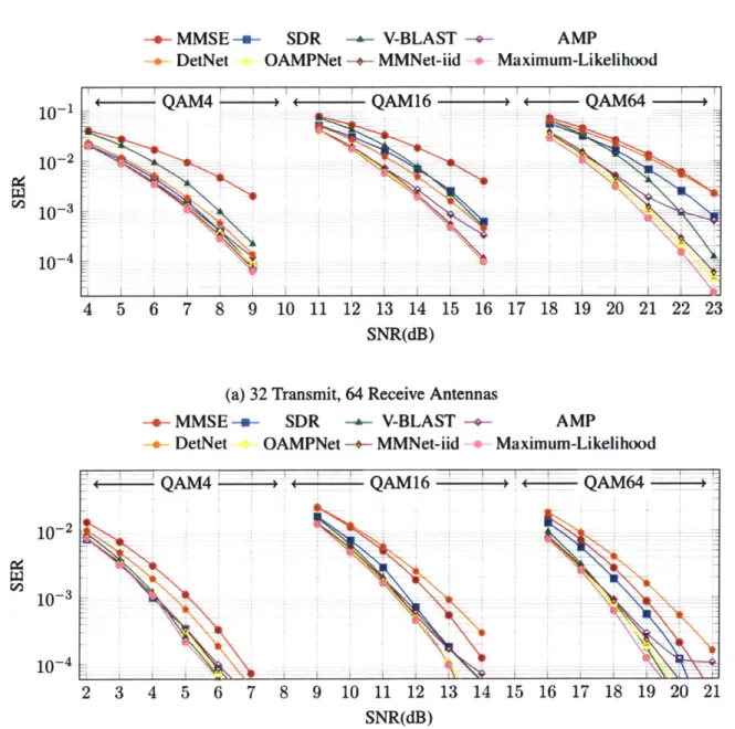
4-1 symbol error rate (SER) vs. signal-to-noise ratio (SNR) of different schemes for three modulations (QAM4, QAM 16 and QAM64) and two system sizes (32 and 16 transmitters, 64 receivers) with i.i.d. Gaussian channels. . . . . 34 4-2 SER vs. SNR of different schemes for three modulations (QAM4, QAM 16

and QAM64) and two system sizes (32 and 16 transmitters, 64 receivers) with 3GPP MIMO channels. . . . 36 4-3 SNR requirement gap with Maximum-Likelihood at SER of 10-3. The total

bar height shows the 90th-percentile gap (over different channels) while the hatched section depicts the average. . . . . 37

5-1 Noise power after the linear and denoiser stages at different layers of OAMP-Net and MMOAMP-Net. The OAMPOAMP-Net denoisers become ineffective after the third layer on 3GPP MIMO channels. . . . 41 5-2 Percentage of transmitters that have Gaussian error distribution after the

linear block for each layer with significance level of 5%. MMNet produces Normal-distributed errors at the output of linear blocks, while OAMPNet fails to achieve the Gaussian property. . . . 42

5-3 Median of Anderson score for the noise at the output of linear stage vs. the power of noise at the input of the stage. MMNet controls the linear block output error distribution to be Gaussian. Dashed horizontal lines show the thresholds for 1%, 5% and 15 significance level. . . . 43

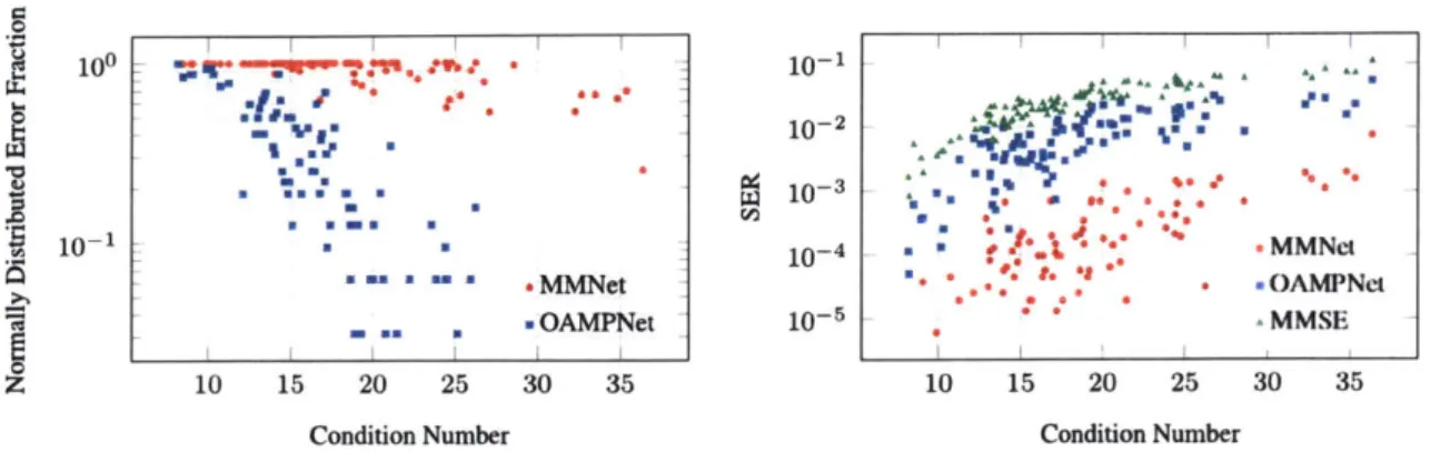
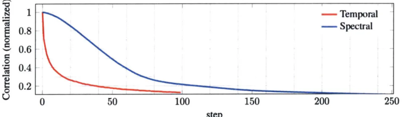
5-4 Effect of condition number on performance of schemes. (a) MMNet is more robust in producing the right noise distribution for denoisers with changes in condition number. (b) SER is directly affected by the condition num ber. . . . 45 6-1 Correlation of channel samples across time and frequency dimensions. The

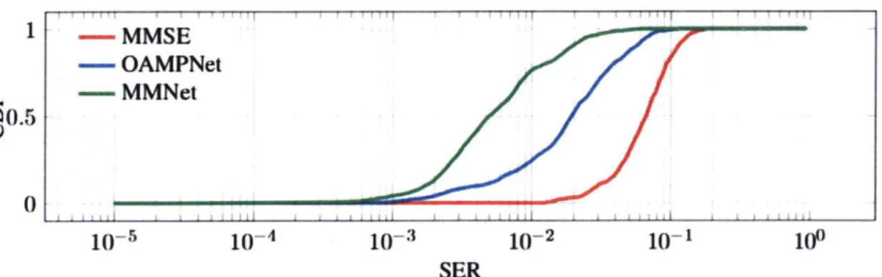
correlation decays relatively quickly in the time dimension, but the channel matrices show strong locality across sub-carriers in frequency dimension. 49 6-2 CDF of SER using Algorithm 1 for training MMNet on QAM16

modu-lation. MMNet requires only 4 overall iterations of batch size 500 per channel realization to train to a reasonable performance. . . . 51 6-3 Number of multiplication operations per signal detection for different

al-gorithms on QAM16 with N, = 64 receive antennas in 3GPP MIMO model. Detection with MMNet, including its online training process, re-quires fewer multiplication operations than detection with pre-trained Det-Net and OAMPDet-Net models. . . . 51

Adaptive Neural Signal Detection for Massive MIMO

by

Mehrdad Khani Shirkoohi

Submitted to the Department of Electrical Engineering and Computer Science on May 24, 2019, in partial fulfillment of the

requirements for the degree of

Master of Science in Computer Science and Engineering

Abstract

Massive Multiple-Input Multiple-Output (MIMO) is a key enabler for fifth generation (5G)

cellular communication systems. Massive MIMO gives rise to challenging signal detection problems for which traditional detectors are either impractical or suffer from performance limitations. Recent work has proposed several learning approaches to MIMO detection with promising results on simple channel models (e.g., i.i.d. Gaussian entries). However, we find that the performance of these schemes degrades significantly in real-world scenar-ios in which the channels of different receivers are spatially correlated. The root of this poor performance is that these schemes either do not exploit the problem structure (re-quiring models with millions of training parameters), or are overly-constrained to mimic algorithms that require very specific assumptions about the channel matrix.

We propose MMNet, a deep learning MIMO detection scheme that significantly outper-forms existing approaches on realistic channel matrices with the same or lower compu-tational complexity. MMNet's design builds on the theory of iterative soft-thresholding algorithms to identify the right degree of model complexity, and it uses a novel training algorithm that leverages temporal and frequency locality of channel matrices at a receiver to accelerate training. Together, these innovations allow MMNet to train online for ev-ery realization of the channel. On i.i.d. Gaussian channels, MMNet requires 2 orders of magnitude fewer operations than existing deep learning schemes but achieves near-optimal performance. On spatially-correlated realistic channels, MMNet achieves the same error rate as the next-best learning scheme (OAMPNet [1]) at 2.5dB lower Signal-to-Noise Ra-tio (SNR) and with at least lOx less computaRa-tional complexity. MMNet is also 4-8dB better overall than a classic linear scheme like the minimum mean square error (MMSE) detector.

Thesis Supervisor: Mohammad Alizadeh

Chapter 1

Introduction

The fifth generation of cellular communication systems (5G) promises an order of magni-tude higher spectral efficiency (measured in bits/s/Hz) than legacy standards such as Long Term Evolution (LTE) [2]. One of the key enablers of this better efficiency is Massive Multiple-Input Multiple-Output (MIMO) [3], in which a base station (BS) equipped with a very large number of antennas (around 64-256) simultaneously serves multiple single-antenna user equipments (UEs) on the same time-frequency resource.

Legacy systems already use MIMO [4], but this is the first time it will be deployed on such a large scale, creating significant challenges for signal detection. The goal of signal detection is to infer the transmitted signal vector x from the vector y = Hx + n received at the BS antennas, where H is the channel matrix, and n is Gaussian noise. Traditional MIMO detection methods with strong performance [5, 6, 7, 8] are feasible only for small systems and have prohibitive complexity for massive MIMO deployments. Thus, there is a need for low-complexity symbol detection schemes that perform well and scale to large

system dimensions.

In recent work, researchers have proposed several learning approaches to MIMO detection. Samuel et al. [9] developed a deep neural network architecture called DetNet with im-pressive performance, e.g., matching the performance of a semidefinite relaxation (SDR)

baseline for i.i.d. Gaussian channel matrices while running 30 x faster. Shortly afterwards, inspired by the Orthogonal AMP algorithm [10], He et al. [I] introduced OAMPNet and demonstrated strong performance on both i.i.d. Gaussian and small-sized correlated chan-nel matrices based on the Kronecker model with exponentially-distributed spatial correla-tions [11]. DetNet and OAMPNet are both trained offline: they try to learn a single model during training for a family of channel matrices (e.g., i.i.d. Gaussian channels). How-ever, the two schemes have different design philosophies. DetNet embeds little domain knowledge into the model and relies on a large neural network with 1-10 million parame-ters depending on the system size and modulation scheme. By contrast, OAMPNet takes a model-driven approach and follows the OAMP algorithm closely; it adds only 2 trainable parameters per iteration of the OAMP algorithm.

In this dissertation we show that neither approach is effective in practice. We conduct extensive experiments using a dataset of channel realizations from the 3GPP 3D MIMO channel [12], as implemented in the QuaDRiGa channel simulator [13]. Our results show that DetNet's training is unstable for realistic channels, while OAMPNet suffers a large performance gap (5-7dB at symbol error rate of 10-3) _{compared to the optimal} Maximum-Likelihood detector on these channels. Both models (as well as several classical baselines) perform well in simpler settings used for evaluation in prior work (e.g., i.i.d. Gaussian channels, low-order modulation schemes). Our results demonstrate the difficulty of learn-ing a fixed detector that generalizes across a wide variety of channel matrices (esp. poorly-conditioned channels that are difficult to invert). DetNet's approach is, in a sense, too general, making the large model difficult to train, while OAMPNet makes strong assump-tions about channel matrices (OAMP was designed for unitarily-invariant channels [10]) and therefore performs poorly on channels that deviate from these assumptions.

Motivated by these findings, we revisit MIMO detection from an online learning perspec-tive. We ask: Can a receiver adapt its detector for every realization of the channel matrix? Such an approach would arguably be simpler and could perform better than a fixed detec-tor that must handle a wide variety of channel matrices. However, conventional wisdom suggests that training a deep neural network online is "impossible" in this context because

of the stringent performance requirements of MIMO detectors [9].

MMNet overcomes this challenge with two key ideas. First, it uses a neural network archi-tecture that strikes the right balance between expressivity and complexity. MMNet's neural network is based on iterative soft-thresholding algorithms [14, 15]. It preserves important aspects of these algorithms in MIMO detection, such as a denoiser architecture tailored for uncorrelated Gaussian noise for different transmitted signals. At the same, MMNet introduces adequate flexibility into these algorithms, with trainable parameters that are op-timized for each channel realization. Second, MMNet's online training algorithm exploits the locality of channel matrices at a receiver in both the frequency and time domains. By leveraging locality, MMNet accelerates training 250 x compared to naively retraining the neural network from scratch for each channel realization. Taken together, these ideas enable MMNet to achieve performance within 1.5dB of the optimal Maximum-Likelihood detec-tor with 10-15 x less computational complexity than the second best scheme, OAMPNet. On random i.i.d. Gaussian channels, we show that a simple version of MMNet with 100 x

less complexity than OAMPNet and DetNet, achieves near-optimal performance without requiring any retraining.

We empirically analyze the dynamics of errors across different layers of MMNet and OAMPNet to understand why MMNet achieves higher detection accuracy. Our analysis reveals that MMNet shapes the distribution of noise at the input of denoisers to ensure they operate effectively. In particular, as signals propagate through the MMNet neural network, the noise distribution at the input of denoiser stages approaches a Gaussian distribution, to create precisely the conditions in which the denoisers can attenuate noise maximally.

The rest of this dissertation is organized as follows. Chapter 2 provides background on classical and learning-based detection schemes, and introduces a general iterative frame-work that can express many of these algorithms. Chapter 3 introduces the MMNet design in addition to a simple variant for i.i.d. channels. Chapter 4 shows performance results of detection algorithms on i.i.d. Gaussian and 3GPP MIMO channels for different mod-ulations. Chapter 5 discusses the error dynamics of MMNet and empirically studies why

it performs better than OAMPNet. Chapter 6 introduces the MMNet online training algo-rithm and how temporal and spectral locality of channel matrices can significantly reduce the computational complexity of training MMNet.

Notation: We will use lowercase symbols for scalars, bold lowercase symbols for vectors and bold uppercase symbols to denote matrices. Symbols {0, 0, 8} are used to represent the parameters of trainable models. The pseudo-inverse of the matrix H is denoted by

Chapter 2

Background and Related Work

This chapter introduces the MIMO detection problem and reviews the most relevant related work.

2.1

Problem Definition

We consider a communication channel from Nt single-antenna transmitters to a receiver equipped with N, antennas. The received vector y E CN is given as

y = Lx + n, (2.1)

where H E CN,xNt is the channel matrix, n ~ C/(O, L.2_{IN,) is complex Gaussian noise}

and x E XN is the vector of transmitted symbols. X denotes the finite set of constellation points. We assume that each transmitter chooses a symbol from X uniformly at random, and all transmitters use the same constellation set. Further, as is standard practice, we assume that the constellation set X is given by a quadrature amplitude modulation (QAM) scheme [16]. All constellations are normalized to unit average power (e.g., the QAM4 constellation is I j }).

(At, bt)

itzt i +

---- linear - denoiser

-Figure 2-1: A block of an iterative detector in general framework. Each block contains a linear transformation followed by a denoising stage.

The channel matrix H is generated by a stochastic process, but it is assumed to be perfectly known at the receiver. The goal of the receiver is to compute the maximum likelihood (ML) estimate of x:

x = arg min I|y - HxI2. (2.2)

XEXNt

The optimization problem in Eq. (2.2) is NP-hard due to the finite-alphabet constraint x E XN [17]. Over the last three decades, researchers have proposed a variety of detectors for this problem with differing levels of complexity. We briefly describe a small subset of existing detection schemes in this chapter. We refer the interested reader to [6, 7] for a comprehensive overview of MIMO detection schemes.

2.2

An iterative framework for MIMO detection

In this dissertation, we focus on a class of iterative estimation algorithms for solving Eq. (2.2) shown in Fig. 2-1. Each iteration of these algorithms comprises the following two steps:

General Iteration: (2.3)

it+1 = it (zt).

The first step takes as input it, a current estimate of x and the received signal y and applies a linear transformation to obtain an intermediate signal zt. In the second step, a non-linear "denoiser" is applied to zt to produce it+,, a new estimate of x that is used as the input for the next iteration. Together, the linear and denoising operations aim to improve the quality

of the estimate Xt from one iteration to the next.

We refer to y - Ht as the residual term. The denoiser qt(-) can be any non-linear function in general; however, most algorithms apply the same thresholding function 3t: C -+ C to each element. Using an element-wise thresholding function can significantly reduce the complexity of the denoising step. Typically denoisers also require one or more scalar parameters which depend on the detector information of the system (channel measurement, residuals, etc.) and they update by each iteration of the algorithm and we denote them by

0

t. We use the terms step, layer and block interchangeably to refer to one complete iteration (the linear step followed by the non-linear denoiser) of the algorithms in this dissertation. All algorithms discussed assume to = 0.

A natural choice for the denoising function is the minimizer of E[II* - x112lzt], which is

given by:

r7(zt) = E[xlzt]. (2.4)

Optimal denoiser for Gaussian noise

Assume that the noise at the input of the denoiser zt - x has an i.i.d. Gaussian distribution with diagonal covariance matrix atN,. The element-wise thresholding function derived from Eq. (2.4) has the form

Of (z; a,2) = x exp

(

where Z = ZX EX exp (- -i). As we see here, o- in Eq. (2.5) denoiser represents the standard deviation of the Gaussian noise on denoiser inputs. In all denoisers in 7j1 (.; ct)

format in this dissertation, o2 refers to the variance of noise in denoiser input.

In the following, we briefly describe several algorithms for MIMO detection. We begin with traditional, non-learning approaches (Q 2.3) and then discuss recent deep learning proposals ( 2.4). We show how many of these algorithms can be expressed in the iterative

framework discussed above.

2.3 Classical MIMO detection algorithms

2.3.1

Linear

The simplest method to approximately solve Eq. (2.2) is to relax the constraint of x E XN to x E CNt and then round the relaxed solution to a point on the constellation:

z = arg min IIY - Hx|2 = Hly,

Linear: XECNt (2.6)

x = arg min I|x -

z112-XEXNt

Rounding each component of z to the closest point in the constellation set x leads to the well-known zero-forcing (ZF) detector, which is equivalent to a single step of Eq. (2.3) with

initial condition of *0 = 0, A₀ = H+, bo = 0 and a hard-decision denoiser with respect to the points in the constellation. Other widely-used single-step linear detectors include the matched filter and the minimum mean square error (MMSE) detectors [3] with A0 = HH

and A₀ = (HH H + (.2

IN,) 1H , respectively. Linear detectors are attractive for practical implementation because of their low complexity, but they perform substantially worse than the optimal detector.

We can also perform the optimization in Eq. (2.6) in multiple iterations using gradient descent. The gradient of the objective function in the first equation of Eq. (2.6) with respect to x is -2HH(y - Hx). Hence, if we set At to 2aHH and bt = 0, the linear step of Eq. (2.3) is equivalent to minimizing

IIy

2.3.2

Approximate Message Passing (AMP)

MIMO detection can, in principle, be solved through belief propagation (BP) if we consider a bipartite graph representation of the model in Eq. (2.1) [18]. BP on this graph requires O(N,Nt) update messages in each iteration, which would be prohibitive for large system dimensions. In the large system limit, Jeon et al. [15] introduce approximate message passing (AMP) as a lower complexity inference algorithm for solving Eq. (2.2) for i.i.d. Gaussian channels. AMP reduces the number of messages in each iteration to O(N, + Nt). The algorithm performs the following sequence of updates:

Zt = *j + HH(y - Hit) + bt,

AMP: b= at (HH(y - Hit_1) + bt_1), (2.7)

it+1 = 7t (zt; at) .

Consider AMP in our iterative framework: we use At = HH as the linear operator. The vector bt is known as the Onsager term. The scalar sequences at and at can be computed given the SNR and system parameters (constellation and number of transmitters and re-ceivers) [19]. The denoising function t (.) applies the optimal denoiser for Gaussian noise in Eq. (2.5) to each element of the vector zt. Jeon et al. [15] prove that AMP is asymptoti-cally optimal for large i.i.d. Gaussian channel matrices.

Orthogonal AMP (OAMP) [10] was proposed for unitarily-invariant channel matrices [20] to relax the i.i.d. Gaussian channel assumption in the original AMP algorithm.

OAMP: zt = Xt + H HHH + a21(y - Hit), (2.8)

Xt+1 = 7t (zt; a2)

In Eq. (2.8), -y, = Nt/trace (V2 HH

(v21HH

AMP.

2.3.3

Other techniques

Several detection schemes relax the lattice constraint (x E XNt) in Eq. (2.2). For example, Semi-Definite Relaxation (SDR) [8] formulates the problem as a semi-definite program. Sphere decoding [5] conducts a search over solutions X such that |y - HiI 12 5 r. In-creasing r covers a larger set of possible solutions, but this comes at the cost of increased complexity, approaching that of brute-force search. There is a large body of variations on improvements to this idea, which can be found in [6, 7]. While these approaches can per-form well, their computational complexity is prohibitive for Massive MIMO systems with currently available hardware.

Another class of detector applies several stages or iterations of linear detection followed by interference subtraction from the observation y. The V-BLAST scheme [21] does this by detecting the strongest symbols, which are then successively removed from y. The drawbacks of this approach are error propagation of early symbol decisions and high com-plexity due to the Nt required stages, as well as the necessary reordering of transmitters after each step. Parallel interference cancellation (PIC) has been proposed to circumvent these problems. PIC jointly detects all transmitted symbols and then attempts to create an interference-free channel for each transmitter through the cancellation of all other trans-mitted symbols [22, 23]. A large system approximation of this approach was recently developed in [24] based on [25]. However, it is currently limited to binary phase shift keying (BPSK) modulation and leads to unsatisfactory performance for realistic system dimensions.

In summary, most existing techniques are too complex to implement at the scale required by next-generation Massive MIMO systems. On the other hand, light-weight techniques like AMP cannot handle correlated channel matrices. These limitations have motivated a number of learning-based proposals for MIMO detection, which we discuss next.

2.4 Learning-based MIMO detection schemes

2.4.1

DetNet

Inspired by iterative projected gradient descent optimization, Samuel et al. [26] propose DetNet, a deep neural network architecture for MIMO detection. This architecture per-forms very well in cases of i.i.d. complex Gaussian channel matrices and achieves the performance of state-of-the-art algorithms in lower-order modulations, such as BPSK and QAM4. However, it is far more complex. The neural network is described by the following

equations:

qt = it_1 - i6)HH + (2)Hy 1,

DetNet: 1 [= 3)q,

+

Vt = _Vt E)(6)Ut + 0(7,t

Xt = _t

where [x]+ = max(x, 0), which is also known as ReLU activation function [27], is applied element-wise.

Although DetNet's performance is promising, it has two main limitations. First, its heuris-tic nature makes it difficult to reason about how the neural network works, and how to extend its architecture, for example, to support spatially correlated channel matrices or higher-order modulation schemes. Second, DetNet's architecture does not incorporate known properties of such iterative methods, and thus it is unnecessarily complex. For ex-ample, many iterative soft-thresholding schemes (including AMP described above) apply a denoiser tailored for Gaussian noise (Eq. (2.5)) independently to each transmitted signal. DetNet's neural network can also be thought to be performing non-linear denoising steps intermixed with linear transformations. However, DetNet's denoisers are fully-connected 2-layer neural networks that operate on the entire vector of transmitted signals, i.e., they are Nt-dimensional functions instead of simple scalar functions.

2.4.2

OAMPNet

He et al. [I] design a learning-based iterative scheme based on the OAMP algorithm. OAMPNet adds two tuning parameters per iteration to the OAMP algorithm. OAMPNet shows very good performance in the case of i.i.d. Gaussian channels, but it does not gener-alize to realistic channels with spatial correlations, as our experiments in Chapter 4 show. The OAMPNet design can be expressed as:

OAMPNet: Zt = Xt + 0')HH (vtHH + 2_{1 -1 (y - Hit) (2.10)} Xt+= Tit (zt; oQ)

OAMPNet uses the same denoisers used by AMP, which are optimal for Gaussian noise. By basing its design on OAMP, OAMPNet makes a strict assumption about the system: unitarily-invariant channel matrices. This reduces OAMPNet to training a few parameters per iteration. However, as our results show, OAMPNet's assumptions make it brittle, and its performance degrades on real channel matrices that do not conform to the assumptions. Further, like OAMP, OAMPNet must compute a matrix pseuo-inverse in each iteration, and therefore its complexity is still quite high compared to schemes like AMP.

Chapter 3

MMNet Design

The MMNet design follows the iterative framework described in 2.2. The main idea behind MMNet is to introduce the right degree offlexibility into the linear and denoising components of the iterative framework while preserving its overall structure. We observe that prior architectures do not strike the right balance between model flexibility and com-plexity. DetNet is very general and expressive, but it requires an enormous number of parameters because it does not incorporate domain knowledge, such as the role and struc-ture of the denoiser in iterative soft-thresholding algorithms. On the other hand, OAMPNet is heavily constrained and follows OAMP very closely; however, OAMP makes rigid as-sumptions about channel matrices (unitarily-invariant channels). Thus, as our results, will show, OAMPNet's performance degrades on real channel matrices that violate this assump-tion.

In practice, not much is known about the distribution of channel matrices. We therefore propose a data-driven approach in which we learn a set of model parameters for each real-ization of H. In this approach, the receiver continually adapts its parameters as it measures new channel matrices H. We demonstrate that this can be realized in practice with a suitable neural network architecture by exploiting the fact that realistic channels exhibit locality in both the frequency and time domains. We introduce the neural network architecture in this chapter and discuss a practical training algorithm in Chapter 6.

We present separate neural network models for (1) i.i.d. Gaussian channels and (2) arbitrary channels. In the i.i.d. Gaussian case, the model is extremely simple:

MMNet-iid: Z = it + (HH(y - Hi)(3.1)

Xt+1 = ?It (zt; o)

Here, the denoiser is the optimal denoiser for Gaussian noise given in Eq. (2.5). MMNet-iid assumes the same distribution of noise at the input of the denoiser for all transmitted symbols and estimates its variance Ot2 according to

O = |III - H|2F

[|ly

The intuition behind Eq. (3.2) is that the noise at the input of the denoiser at step t is comprised of two parts: (1) the residual error caused by deviation of it from the true value of x, and (2) the contribution of the channel noise n. The first component is amplified by the linear transformation (I - AtH), and the second component is amplified by At. See [10, 15] for further details on this method for estimating noise variance.

This model has only two parameters per layer: t 1 and 6 .We discuss this model merely

to illustrate that, for the i.i.d. Gaussian channel matrix case (which most prior work has used for evaluation), a simple model that adds a small amount of flexibility to existing algorithms like AMP can perform very well. In fact, our results will show that, in this case, we do not even need to train the parameters of the model online for each channel realization; training offline over randomly sampled i.i.d. Gaussian channel suffices.

The MMNet neural network for arbitrary channel matrices is as follows: M t = i + 801)(y - Hit),

MMNet: t(3.3)

it+1 = 7t (zt; o)

In Eq. (3.3), 8(l) is an Nt x N, complex-valued trainable matrix. In order to enable the model to handle cases in which different transmitted symbols have differing levels of noise,

we add an extra degree of freedom to our estimations of noise per transmitter, resulting in:

S(2) - AtHII2 2+

AtI|(

2 t

II-AHF

[Ily

_HitII

(Tt = Nt |H11} 2 2l| -r(,.2] + + IIHI12F 2 (3.4)

Parameter vector 0(2) of size Nt x 1 scales the noise variance by different amounts for each

symbol. This approach distinguishes MMNet from both the highly-constrained OAMPNet and overly complex DetNet solution. In particular, MMNet uses a flexible linear transfor-mation (which does not need to be linear in H) to construct the intermediate signal zt, but it applies the standard optimal denoiser for Gaussian noise in Eq. (2.5). Further, unlike OAMPNet, MMNet does not require any expensive matrix inverse operation.

MMNet concatenates T layers of the above form. We use the the average L2-loss over all T layers in order to train the model. This loss is denoted by L in Eq. (3.5).

T

L= 11it - x11. (3.5)

J

Chapter 4

Experiments

In this chapter, we evaluate and compare the performance of MMNet with state-of-the-art schemes for both i.i.d. Gaussian and realistic channel matrices. These are our main findings:

1. On i.i.d. Gaussian channels, most schemes perform very well. MMSE, SDR, V-BLAST and DetNet are 1-2dB far from the best schemes overall. AMP performance degrades for higher-order modulations in high SNRs. MMNet-iid and OAMPNet are very close to Maximum-Likelihood in all experiment on these channels. MMNet-iid, however, has 2 orders of magnitude lower complexity than learning-based schemes OAMPNet and DetNet.

2. On realistic, spatially-correlated channel matrices, the performance of all existing learning-based approaches degrades significantly. MMNet shows the least gap with Maximum-Likelihood in all schemes. While DetNet and AMP fail to extend to these channels with reasonable performance (on QAM4, for example), MMSE has an 8-10dB gap with Maximum-Likelihood on 64 x 16 channels. OAMPNet reduces this gap to 5-7dB. However, MMNet closes the gap to less than 1.5dB.

4.1 Methodology

We first briefly discuss the details of detection schemes used for comparison. Since some of these schemes (including MMNet) require training, we then discuss the process of gen-erating data and training/testing on this data.

4.1.1

Compared Schemes

In our experiments, we compare the following schemes on QAM modulation:

* MMSE: Linear decoder that applies the SNR-regularized channel's pseudo inverse and rounds the output to the closest point on the constellation (see 2.3.1).

" SDR: Semidefinite programming using a rank- 1 relaxation interior point method [28]. " V-BLAST: Multi-stage interference cancellation BLAST algorithm using Zero-Forcing

as the detection stage introduced in [23].

" AMP: AMP algorithm for MIMO detection from Jeon et al. [15]. AMP runs 50

iterations of the updates as discussed in Eq. (2.7). We verified that adding more iterations does not improve the results.

* DetNet: The deep learning approach introduced in [26]. The DetNet paper describes instantiations of the architecture for BPSK, QAM4 and QAM16; these neural net-works have, on the order of 1-1 OM, trainable parameters depending on the size of the system and constellation set.

" OAMPNet: The OAMP-based architecture [1] implemented in 10 layers with 2 trainable parameters per layer and an inverse matrix computation at each layer. * MMNet-iid: The simple architecture described in Chapter 3. This scheme has only

2 scalar parameters per layer and does not require any matrix inversions. We imple-ment this neural network with 10 layers.

* MMNet: Our design described in Eq. (3.3). It has 10 blocks, and the total number of trainable parameters is 2Nt(N, +1) real values, independent of constellation size. " Maximum-Likelihood: The optimal solver for Eq. (2.2) using a highly-optimized

Mixed Integer Programming package Gurobi [29].

4.1.2 Dataset

Training and test data are generated through the model described in Eq. (2.1). In this model, there are three sources of randomness: signal x, channel noise n and channel matrix H. Each transmitted signal x is generated randomly and uniformly over the corresponding constellation set. All transmitters are assumed to use the same modulation. The channel noise n is sampled from a zero-mean i.i.d. normal distribution with a variance that is set according to the operating SNR, defined as SNR(dB) = 10 log (E[IIHxI2]/E[jnjj']). For every training batch, the SNR(dB) is chosen uniformly at random in the desired operating SNR interval. This interval depends on the modulation scheme. For each modulation in each experiment, the SNR regime is chosen such that the best scheme other than Maximum-Likelihood can achieve a SER of 10~3-10-2.

The channel matrices H are either sampled from an i.i.d. Gaussian distribution (i.e., each column of H is a complex-normal CAf(0, (1/N,)IN,,)), or they are generated via the realistic channel simulation described below.

Here, we study two system size ratios (Nt/N,) of 0.25 and 0.5, with the total number of re-ceivers fixed at N, = 64. These are typical values for 4G/5G base stations in urban cellular deployments. For the case of realistic channels, we generate a dataset of channel realiza-tions from the 3GPP 3D MIMO channel model [12], as implemented in the QuaDRiGa channel simulator [13].' We consider a base station (BS) equipped with a rectangular pla-nar array consisting of 32 dual-polarized antennas installed at a height of 25 m. The BS is assumed to cover a 120*-cell sector of radius 500 m within which Nt E

{16,

antenna users are dropped randomly. A guard distance of 10 m from the BS is kept. Each user is then assumed to move along a linear trajectory with a speed of 1 m/s. Channels are sampled every A/4 m at a center frequency of 2.53 GHz to obtain sequences of length 100. Each channel realization is then converted to the frequency domain assuming a bandwidth of 20 MHz and using 1024 sub-carriers from which only every fourth is kept, resulting in F = _{256 effective sub-carriers. We gather a total of 40 user drops, resulting in 40 x 256} length 100 sequences of channel matrices (i.e., 1M channel matrices in total). Since the pathloss can vary dramatically between different users, we assume perfect power control, which normalizes the average received power across antennas and sub-carriers to one. De-note H[f, k] as the kth column of channel matrix on sub-carrier

_f.

1 Nt F

N,NtFEZ Z H[fk]|=2 k=1 f=1

4.1.3

Training

MMNet, DetNet, and OAMPNet require training and were implemented in TensorFlow [30]. We have converted Eq. (2.2) to its equivalent real-valued representation for TensorFlow im-plementations (cf. [31, Sec. II]). DetNet and OAMPNet are both trained as described in the corresponding publications (i.e., batch size of 5K samples). We trained each of the latter two algorithms for 50K iterations.

To train MMNet, we use the Adam optimizer [32] with a learning rate of 10-3. Each training batch has a size of 500 samples. We train MMNet for 1K iterations on each real-ization of H in the naive implementation. In 6.2, we exploit frequency and time domain correlations to reduce the training requirement to 4 iterations per channel matrix.

For i.i.d. Gaussian channels, MMNet-iid is not trained per channel realization H. Instead, we use 10K iterations with a batch size of 500 samples to train a single MMNet-iid neural network, which we then test on new channel samples.

4.2 Results

We compare different schemes along two axes: performance and complexity. In this sec-tion, we focus on performance, leaving a comparison of complexity to Chapter 6. We use the SNR required to achieve an SER of 10- as the primary performance metric. In

practice, most error correcting schemes operate around a SER of 10-3-10-2, so this is the

relevant regime for MIMO detection.

4.2.1

i.i.d. Gaussian channels

Fig. 4-1 shows the SER vs. SNR of the state-of-the-art MIMO schemes on Complex-Gaussian i.i.d. channels for two system sizes: 32 and 16 transmitters (Fig. 1a and Fig.

4-1 b, respectively).

We make the following observations:

1. The SNR required to achieve a certain SER increases by 2-3dB as we double the number of transmitters (notice the different range of x-axes). The reason is that there is higher interference with more transmitters.

2. There is a 2-3dB performance gap between Maximum-Likelihood and MMSE across all modulations for Nt = 32. However, this gap decreases to 1dB for Nt = 16, because received signals have lower interference in this case.

3. Multiple schemes perform similarly to Maximum-Likelihood, especially at lower-order modulations like QAM4. As we move to QAM64, the performance of several schemes degrades compared to Maximum-Likelihood.

4. SDR performs better than MMSE, but its gap with Maximum-Likelihood increases with modulation order.

-*- MMSE --- SDR --- V-BLAST -+-+ DetNet 10-1 10~2 GO10-3 10-4 10-2 10- 3 10-4

OAMPNet -+- MMNet-iid # Maximum-Likelihood

QAM4

QAM64

4 5 6 7 8 9 10 11 12 13 14 15 16 17 18 19 20 21 22 23

SNR(dB)

(a) 32 Transmit, 64 Receive Antennas

-+- MMSE -m- SDR --- V-BLAST -+- AMP

-. DetNet OAMPNet -+- MMNet-iid * Maximum-Likelihood

QAM14 QAM16 QAM64

2 3 4 5 6 7 8 9 10 11 12 13 14 15 16 17 18 19 20 21 SNR(dB)

(b) 16 Transmit, 64 Receive Antennas

Figure 4-1: SER vs. SNR of different schemes for three modulations (QAM4, QAM16 and QAM64) and two system sizes (32 and 16 transmitters, 64 receivers) with i.i.d. Gaussian channels.

have 16 transmit antennas. However, its performance is sensitive to system size and degrades when we increase the number of transmitters to 32.

6. AMP is near-optimal in many cases (recall that, theoretically, AMP is asymptotically optimal for i.i.d. Gaussian channels). However, it suffers from robustness issues at higher SNR levels, especially with higher-order modulations like QAM64.

7. DetNet has a good performance on QAM4, but its gap with Maximum-Likelihood increases as we move to QAM16 and QAM64. With QAM64, DetNet performs even worse than MMSE for Nt = 16.

8. OAMPNet and the simple MMNet-iid approach are both very close to Maximum-Likelihood across different modulations over a wide range of SNRs, even though these models have only two parameters per layer. Unlike OAMPNet, MMNet-iid does not require any matrix inversions. As we discuss in Chapter 6, MMNet-iid has O(N,) x lower computational complexity than OAMPNet because it does not need matrix inversions and must learn only 20 parameters in total, compared to the more than IM trainable parameters of DetNet.

In summary, these results show that for i.i.d. Gaussian channel matrices, adding just a small amount of flexibility via tuning parameters to existing iterative schemes like AMP can re-sult in equivalent or improved performance over much more complex deep learning models like DetNet. These models may even outperform classical algorithms like SDR.

4.2.2 Realistic channels

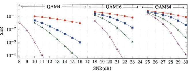
Fig. 4-2 shows the results for the realistic channels derived using the 3GPP 3D MIMO chan-nel model. We consider only MMSE (as a baseline), OAMPNet, MMNet and Maximum-Likelihood. As shown in the i.i.d. Gaussian case, schemes like SDR, V-BLAST and DetNet do not perform as well as the OAMPNet baseline.2 Also, AMP is not designed for

corre-2_{We tried to train DetNet for realistic channels and ran into significant difficulty with stability and}

-+- MMSE -a- OAMPNet -- MMNet -+- Maximum-Likelihood

8 9 10 11 12 13 14 15 16 17 18 19 20 21 22 23 24 25 26 27 28 29 30

SNR(dB)

(a) 32 Transmit, 64 Receive Antennas

-- MMSE -- OAMPNet -A- MMNet -+- Maximum-Likelihood

4 5 6 7 8 9 10 11 12 13 14 15 16 17 18

SNR(dB)

19 20 21 22 23 24 25

(b) 16 Transmit, 64 Receive Antennas

Figure 4-2: SER vs. SNR of different schemes for three modulations (QAM4, QAM16 and

QAM64) and two system sizes (32 and 16 transmitters, 64 receivers) with 3GPP MIMO

channels.

QAM4 QAM16 - --- QAM64 -- L--+

10-1 @ 10-2

con

L I MMSE ROAMPNet MMNet

S15 15

10 10

5 L5

i MMSE OAMPNet [ MMNet

0

-QAM4 QAM16 QAM64 o QAM4 QAM16 QAM64

Modulation Modulation

(a) 3GPP MIMO Nt = 16 (b) 3GPP MIMO Nt = 32

Figure 4-3: SNR requirement gap with Maximum-Likelihood at SER of 10- 3. The total bar height shows the 90th-percentile gap (over different channels) while the hatched section depicts the average.

lated channels and is known to perform poorly (see discussion in chapter 5).

We make the following observations:

1. There is a much larger gap with Maximum-Likelihood for all detection schemes on

these channels compared to the i.i.d. case.

2. We require 4-7dB increase in the SNR ranges relative to Fig. 4-1. Also, doubling the number of transmitters from Fig. 4-2b to Fig. 4-2a costs about 5dB in SNR for each

scheme this time (compare with 2-3dB in i.i.d. case.)

3. MMSE as a baseline shows a relatively flat SER vs. SNR in this case. For example,

it requires 5dB SNR improvement on QAM16 to go from an SER of 2% to 1%.

4. OAMPNet performance improvement slope is faster than MMSE. It shows 2-3dB average improvement in SNR requirement relative to MMSE to achieve the same

SER.

5. MMNet outperforms MMSE and OAMNet schemes for both system sizes and in all

modulations.

detec-j1

tion schemes. For this purpose, we measure the difference in the minimum SNR level that is required to have SER of 10-3. In this figure, we have also attempted to show the variabil-ity of this requirement across different channel situations by adding the 90th-percentile gap over different channel conditions. We observe that MMNet can achieve up to 5dB and 8dB improvement, respectively, over OAMPNet and MMSE on more realistic channels.

Chapter

5

Why MMNet works

In this chapter, we examine why MMNet performs better than other schemes. By analyzing the dynamics of the error (it - x), we find that MMNet's denoisers are significantly more effective than those in OAMPNet. We show that this occurs because MMNet's linear stages control the distribution of noise at the input of the denoisers. Specifically, MMNet ensures that the noise input to the denoisers is nearly Gaussian, whereas the noise distribution for OAMPNet is far from Gaussian. Since the denoisers in both architectures are tailored for Gaussian noise, they perform much better in MMNet.

5.1

Error dynamics

Define the error at the outputs of the linear and denoiser stages at iteration t as e = Zt -X

and eden = kt+i - x, respectively. For algorithms such as MMNet and OAMPNet where bt = 0, We can rewrite the update equations of Eq. (2.3) in terms of these two errors in the form:

ei (I -AtH)e ' = + Atn, (5.1a)

Eq. (5.1 _{a) includes two terms, corresponding to the contribution of the error of the previous} stages' output and the channel noise to ef respectively. To gain intuition, consider the effect of several choices of At.

If we set At to H+ (the pseudo-inverse of the channel matrix), we are only left with the term H+n in e'", thus eliminating the error caused by the previous stage entirely. However, this comes at a price: we are left with Gaussian noise with covariance matrix 0,2H+H+H. This

presents two potential problems: (1) if H is ill-conditioned, it might amplify the channel noise (e.g., inversely proportional to the smallest singular value of H in some directions); (2) if el" _{is correlated noise, applying an element-wise denoising function to it may not be}

effective.

We could also remove the channel noise term entirely by setting At to zero. This would effectively remove the linear stage. However, if optimal denoisers are used, removing the linear stage and applying the denoiser function twice should have no effect on reducing the error.

For i.i.d. Gaussian channels with variance 1/N,, if we set At = HH, the factor I - AtH asymptotically goes to zero as we increase N, [19]. The auto-covariance of Atn, U2_HHH,

is approximately equal to a21N,. _{This means that the channel noise term is neither amplified}

nor correlated following this linear transformation with i.i.d. channels, while the error from the previous stage, et, is attenuated significantly via I - AtH. These calculations explain why AMP has great performance on i.i.d. Gaussian channels. However, in case of correlated channels, neither I - _{AtH is close to zero, nor is Atn uncorrelated. This is the} primary reason that AMP cannot perform well on more realistic channels.

5.2

Analysis

As noted earlier, the key element in MMNet and prior schemes such as OAMPNet is how to pick the linear transformation At. Based on the above discussion of the error dynamics,

0.2 -- MMNel after linear

- @- MMNet after denoiser

0.15 OAMPNet after linear

- U- OAMPNet after denoiser

4) 0.1

0.05

0 -- --- ---- ~0

-0 1 2 3 4 5 6 7 8 9

Layer number (t)

Figure 5-1: Noise power after the linear and denoiser stages at different layers of OAMPNet and MMNet. The OAMPNet denoisers become ineffective after the third layer on 3GPP MIMO channels.

we identify two desirable properties:

1. At must reduce the magnitude of et". This requires striking a balance between the two terms in Eq. (5.1 a), because attenuating one term may amplify the other and vice-versa.

2. At must "shape" the distribution of el" to make it suitable for the subsequent de-noiser. In particular, the denoisers in most iterative schemes (e.g., MMNet and OMAPNet) are specifically designed for i.i.d. Gaussian noise. Thus, ideally, the linear stage should avoid outputting correlated or non-Gaussian noise.

Fig. 5-1 shows the average noise power at the output of the linear and denoiser stages across iterations, for both OAMPNet and MMNet on 64 x 16 3GPP MIMO channels. The average noise power before and after the denoiser saturate at the same value in OAMPNet from the third layer (t = 2) onwards, showing that the denoisers are no longer effective after a few iterations.

We hypothesize that the reason OAMPNet's denoisers become ineffective is that the noise distribution for OAMPNet is not Gaussian, whereas MMNet is able to provide near-Gaussian noise to its denoiser. We evaluate how close the noise distribution is to Gaussian for both schemes using the Anderson test [33]. In order to measure this score, we generate 10,000 samples per channel realization H. We then calculate the Anderson score for the noise dis-tribution at each linear stage output per transmitter, and per channel matrix. If this score is

0.9 0.8 -0.7 S 0.6 0.5 -- MMNet 0.4 -0- OAMPNet 0.3 0.2 0.1 --0 0 1 2 3 4 5 6 7 8 9 Layer number (t)

Figure 5-2: _{Percentage of transmitters that have Gaussian error distribution after the linear}

block for each layer with significance level of 5%. MMNet produces Normal-distributed errors at the output of linear blocks, while OAMPNet fails to achieve the Gaussian property. below a threshold of 0.786, it indicates that the noise comes from a Gaussian distribution with a significance of 5%, i.e. the probability of false rejection of a Gaussian distribution is less than 5%.

In Fig. 5-2, _{we plot the average ratio of transmitters that have Normally-distributed noise at}

the output of the linear stage according to this test. Since in both schemes we start with ^0 = 0, the output of the linear stage at layer t = _{0 is Aon, which is Gaussian. Thus, the fraction}

of transmitters with Gaussian noise is 1 in layer t = 0 for both schemes. However, both schemes deviate from Gaussian noise in layer t = 1 while sharply reducing the total noise power as seen in Fig. 5-1. However, MMNet deviates less from a Gaussian distribution. Unlike OAMPNet, in which the noise for 95% of the transmitters is not Gaussian at layer t = _{1, for MMNet nearly 40% of the transmitter exhibit Gaussian noise. On the other hand,}

MMNet reduces the noise power slightly less than OAMPNet in layer t = 1.

In subsequent layers, the noise distribution for MMNet becomes increasingly Gaussian, with nearly 90% of transmitter passing the Anderson test by layer t = 9. By contrast, most transmitters in OAMPNet continue to exhibit non-Gaussian noise in subsequent layers, though the fraction of transmitter with Gaussian noise increases marginally.

Next, we measure the effect of input error power on the output error distribution of linear stages in both schemes. In other words, we are interested to know how

Ie

count in bin 5 10 15 102: MN EME ase mi 101 m a.. 1 A. - -- ---i -0-1 10-3 10-2 10-1 Ie den _t-1 I_| 0 Q 0 count in bin 0 10 20 30 40 102 101: 100 10- ----- 10-1, ... 10-3 10-2 10-1 leden _St-11I

(a) OAMPNet (b) MMNet

Figure 5-3: Median of Anderson score for the noise at the output of linear stage vs. the power of noise at the input of the stage. MMNet controls the linear block output error distribution to be Gaussian. Dashed horizontal lines show the thresholds for 1%, 5% and

15 significance level. 0 0 cp, 0 0-C#0

Gaussian distribution property of el". For this purpose, we choose the median of Anderson scores as a measure of the linear stage's ability to control the distribution of its output errors. In Fig. 5-3, _{we show the 2D histogram of this median score for different values of}

Iedi

test with dashed horizontal lines as a reference. To be Normally distributed with 1%, 5%, or 15% confidence, the Anderson scores must fall below the respective line.

We notice that the median score in both schemes increases with the norm of the error from the previous denoiser stage. In other words, the linear stages that have a higher input noise power produce outputs that deviate more from Gaussian noise. However, MMNet is 100 x

better in terms of the median score at controlling the input error for large value of I|et" 11. This figure also suggests that the poor performance of OAMPNet in final layers is likely not only because of the aggressive approach it has taken at t = 1. Later linear stages are also not very good at controlling the distribution of their output errors.

5.3

_{Impact of channel condition number}

Finally, we evauate the impact of the channel condition number on MMNet and OAMP-Net. A channel's condition number is defined as the ratio of its largest singular value to the smallest. It is well-known to be more difficult to detect signals passing through channel ma-trices with higher condition numbers, as received signals belonging to different transmitted signals can be hard to distinguish passing through such channels.

OAMPNet tries to address this issue by introducing filtering over the singular values. In fact, the linear update equation in Eq. (2.10) attempts to map each singular value s in H to s/ 2+ o). _{This in turn attempts to dynamically adjust the shape of the sphere}

mapping in each iteration by tuning 0(1) and V2. We see that if all singular values are near

each other, as is usually the case in i.i.d. Gaussian channels, OAMPNet easily maps each sphere of signals in the transmit space to a non-skewed sphere in the receive signals space. However, our results show that manipulating the singular values is not the best option for

" 10-2 d; - A --i 1a- a a 10-3 - so . M e -. t" . .OAMPNct M so .OAMPNet - 10-5 : MMSE z 10 15 20 25 30 35 10 15 20 25 30 35

Condition Number Condition Number

(a) Ratio of el" Gaussians vs. channel condition (b) SER on 3GPP MIMO channels

number

Figure 5-4: Effect of condition number on performance of schemes. (a) MMNet is more robust in producing the right noise distribution for denoisers with changes in condition number. (b) SER is directly affected by the condition number.

poorer channel condition numbers.

In Fig. 5-4a, we show the scatterplot of performance of MMNet linear stage in terms of preserving the Gaussian distribution property of their output error distribution across dif-ferent channel condition numbers sample from our 3GPP MIMO dataset after a few initial iterations (t = 4). We see that the fraction of Normally-distributed errors decreases quickly for OMAPNet with the increase in condition number, while MMNet maintains the ratio for a broader range of condition numbers in 3GPP MIMO channels. The consequence of this failure in meeting the underlying assumptions of the model shows up in Fig. 5-4b. In this figure, we show the scatterplot of SER at different condition numbers for 3GPP MIMO channels. Although all schemes' performances are affected by the condition number, MM-Net can almost maintain an SER of around 10-3 almost across all conditions.

4

Chapter 6

Online Training Algorithm

Training deep-learning models is a computationally intensive task, often requiring hours or even days for large models. The computation overhead depends on two factors: (i) the total number of required training samples, and (ii) the size of the model. For example, in training a model like DetNet with order of IM parameters, we need 50K iterations with a batch size of 5K samples, i.e., 250M training samples. If we assume each parameter of the model shows up in at least one floating-point operation per training sample, we require a minimum of 2.5 x 1014 floating-point operations for the entire process of training DetNet. This extreme computational complexity makes training such models online for each realization of H all but impossible.

By contrast, MMNet has only -40K parameters, and training it from scratch requires about 1000 iterations with batch size of 500. Further, this chapter will show that by taking advan-tage of locality of the channels observed at a receiver, we can effectively train the model for each channel realization in 4 iterations (with batch size 500) on average. Thus train-ing MMNet has 6 orders of magnitude lower computational overhead than DetNet, maktrain-ing online training for each realization of H practical.

In this chapter, we first discuss the temporal and spectral locality of 3GPP MIMO channels. Next, we show how we can exploit these localities to accelerate online training.