Fundamental Stokes eigenmodes in the square: which expansion is more accurate, Chebyshev or Reid-Harris?

(1)

Numerical Algorithms (2005) 38:111-131 9 Springer 2005

Fundamental Stokes eigenmodes in the square: which

expansion is more accurate, Chebyshev or Reid-Harris?

E. Leriche and G. Labrosse *

Laboratoire d'Ing~nierie Num~rique, lnstitut des Sciences de l'Energie,

Facult~ des Sciences et Techniques de l'Ing~nieur, Ecole Polytechnique F~d~rale de Lausanne, CH-1015 Ecublens, Switzerland

E-mail: emmanuel.leriche@epfl.ch, labrosse@limsi.fr

Received 10 April 2003; accepted 12 December 2003

The well-known Reid-Harris expansions, applied to the stream function formulation, and the projection-diffusion Chebyshev Stokes solver, in primitive variables, are used to compute the fundamental Stokes eigenmodes of each of the symmetry families characterizing the Stokes solutions in the square. The numerical accuracy of both methods, applied with several discretizations, are compared, for both the eigenvalues and the main features of the corresponding eigenmodes. The Chebyshev approach is by far the most efficient, even though the associated solver does not provide a divergence free velocity but asymptotically.

Keywords: Stokes eigenmodes, Chebyshev and Reid-Harris spectral methods AMS subject classification: 76M22, 76D07

1. Introduction

The Cartesian Stokes eigenmodes are not analytically known except when they are periodic in all, or in all but one, space directions. If they are indeed constrained to verify no-slip velocity conditions on a closed boundary they can only be determined by numerical approach. The present paper regards the Stokes fundamental eigenmodes in the square whose physical implications are commented in [ 12] and illustrated in [5,6,22], for instance. Only one of them is known to the authors' knowledge, the most fundamental of all, whose symmetry properties are the most straightforwardly expected [5,22]. All symmetry configurations are reported in this paper.

Computing the Stokes eigenmodes can be made from either their (velocity- pressure) primitive variable or stream function formulation, but the choice of the scheme is particularly relevant. With the former formulation, the well-known Stokes solvers are either non consistent, namely the time-splitting schemes, or very expensive, even for the 2D present case, namely the Uzawa and Green (or influence matrix) options. On * On leave from Universit6 Paris-Sud, LIMSI-CNRS, BP 133, 91403 Orsay Cedex, France.

(2)

112 E. Leriche, G. Labrosse / Fundamental Stokes eigenmodes in the square

the stream function formulation side, it is worth mentioning here that the biorthogonal series based on "Papkovich-Fadle" polynomial expansions [7,17,19] cannot be used for solving this problem. They lead indeed to a transcendental eigenvalue system, the matrix entries depending on the eigenvalue to be evaluated [20]. Moreover one of the problems raised by the eigenmodes accurate numerical determination regards the requirement of enforcing the numerical velocity to be divergence free for obtaining relevant and conver- gent results.

The present contribution has opted for using two different spectral expansions, associated with each Stokes formulation: a Chebyshev collocation method and the Galerkin-Reid-Harris (RH) decomposition. The former one feeds a pseudospectral solver in primitive variables (the Projection-Diffusion (PrDi)) known to be consistent with the continuous space-time problem [ 11 ], and optimal in computation cost. The lat- ter one uses the well known eigenmodes of the fourth-order differential problem [9,15], completed with no-slip/no-flux boundary conditions, for solving the stream function formulation. This problem is known in structural mechanics as being the buckling load problem [16,21]. These approaches differ intrinsically, as regards, for instance, the numerical velocity divergence which asymptotically vanishes with the polynomial degree in the former case, while it is exactly zero in the second one.

The paper is organized as follows. Section 2 provides the governing equations. The Stokes eigenmodes in the square enjoy symmetry properties. They are exposed in section 3. Then both numerical approaches are presented in section 4. Section 5 brings the results for the fundamental mode of each symmetry family. A systematic comparison is made of the converging behaviors and numerical accuracy that each approach supplies for the eigenvalue and eigenmodes main features. A conclusion terminates this contribution.

2. Governing equations

Let us consider the dimensionless formulation of the 2D Stokes eigenproblem, written in the open domain g2 = ] - 1 , 1[ 2 with coordinates x = (x, y) = (xl, x2) and (u, p) = ((u, v), p) the velocity and pressure eigenmode:

,ku= A u - Vp forx 6 f2, (1)

V 9 u = 0 for x 6 ~ , (2)

u = 0 for x 6 Of2, (3)

where ~. is the Stokes eigenvalue. We denote the closure of ~2 by f2 and the boundary by Of 2.

The (u, p) uncoupled version reads

( ~ - A ) A u = 0 f o r x r ~ , (4)

(3)

E. Leriche, G. Labrosse / Fundamental Stokes eigenmodes in the square 113 x \ \ x x \ x a ~ , A e y

M

~ Y ", f 0

x,

" ' , . " ' "

M

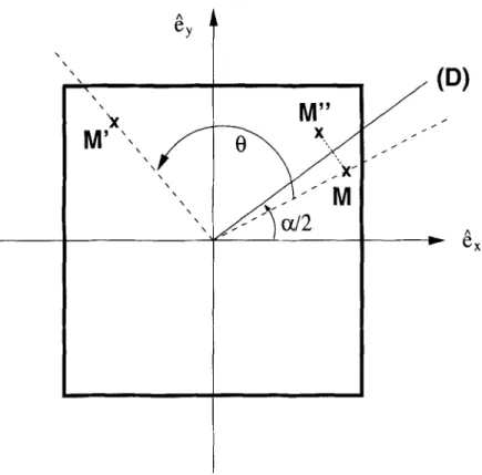
A e x

Figure 1. The 0-rotation and the u-mirror-symmetry about the (D) line making an angle ~/2 with e.r. The stream function formulation, known as the buckling load problem, with ~ (x) such that (u, v) =

(O~/Oy, -O~/Ox),

is

( X - A ) A ~ t = O f o r x 6 f 2 , (6) with

~p-- - - 0 f o r x 6 0 f 2 , (7)

On

n being the coordinate evaluated along n, the unit vector normal to ;9f2.

3. Symmetries

Apart from the translation which is not of interest here, two planar isometries are to be considered [18]: the 0-rotation around the square center, and the a-symmetry, that is the mirror-reflection about the straight line (D) making an a / 2 angle with the unit horizontal axis ex. These transformations are sketched in figure 1, with M = (x, y) M' = (x', y') under the application of a 0-rotation, and M = (x, y) --+ M" = (x", y") under an a-symmetry. Corresponding operators are introduced, respectively denoted by

R(O)

and 8(~). They describe the transformation of any function ~(x, y), with

(4)

114 E. Leriche, G. Labrosse / Fundamental Stokes eigenmodes in the square

~(x', y') =

T4(O)~(x, y)

and ~(x", y ' ) =

S(u)~(x, y).

Because of the square geom- etry, 0 and ot must be integer multiples of rr/2 and only the R ( m r / 2 ) and

S(nJr/2)

operators, n being integer, are to take into account.

Composition rules are easy to establish, for instance, 7"~(01)']~(02) = "~(01 q-- 02) ,

~ ( o ) S ( a ) = S(O + a ) , S(a)T4(O) = S ( a - 0),

S ( O l l ) S ( o r : ']~(or 1 _ or2).

From them it can be shown that all possible transformations can be generated by only three isometries. The common eigenmodes of ~(rr), 74(zr/2) and S(0) are then chosen for spanning the functional space of any Stokes solution. Let us note lYl, n , }'3) these eigenmodes thus defined by the following three relations,

~Ur)l• m, • = }',[gl, m, • ~ 11, n , n ) = n i l , n , n ) , S(0)I• }2, }3> = h i • re, n>,

in which we have >'1 = + 1, }'3 = -4-1 and n = + 1 only with }'1 = 1. The }'1 = - 1 states have no 7Z(zr/2) symmetry. They are denoted by I - 1 , / , + l ) . Together with the I1, +1, +1) states, we have therefore 6 symmetry families for classifying the Stokes solutions. Those having given n and }'3 are also eigenmodes of S((2n + 1)Jr/2), rep- resenting reflection about the square diagonals with

}'2}'3

as eigenvalue. Therefore, in contrast with the others, the families I - 1 , / , + 1) have no reflection symmetry about the square diagonals. Finally, from the relations

it is inferred that the Stokes eigenmodes which are odd under the rr-rotation appear by pair associated with the same eigenvalue.

These eigenmodes have to be identified, family per family, within the numerical solutions of the projection-diffusion Stokes solver, whereas their analytical formulation has to be build for solving the buckling load biharmonic problem.

4. Solvers

This section gathers the main features of both discrete eigenproblems, the primitive variables projection--diffusion solver and the stream function Reid-Harris system.

4.1. Chebyshev projection-diffusion Stokes solver

The uncoupling between the velocity and pressure fields is the major difficulty of any primitive variables approach. In particular, the continuous uncoupled problem given by equations (4), (5) cannot be the starting point of any discrete system since it requires

(5)

E. Leriche, G. Labrosse / Fundamental Stokes eigenmodes in the square 115 twice as many boundary conditions on velocity as available. Therefore, the consistent [11 ] continuous uncoupled formulation is first introduced followed then by the key points of its discrete version, whose details are presented in [1 1].

4.1.1. The continuous projection--diffusion uncoupling

The PrDi solver performs a (u, p) uncoupling by introducing from equations (1), (2) an intermediate divergence free field, the acceleration a,

a = ku - A u , (8)

leading to solve the problem into two steps.

1. The pressure is evaluated from the following Darcy problem:

a + V p = 0 i n f 2 , , i = 1 , 2 , (9)

V . a = 0 in S2, (10)

a . n = ( V x V x ) u . n onOf2. (11)

The f2, are defined by

~"~1 = ] - 1 , - q - l [ x [ - 1 , + l ] , ~22 = [ - I , --F1] x ] - 1 , q--l [,

respectively for the first and second components of (9). The normal boundary condition (11) takes into account equation (8) together with the boundary condition (3) and the incompressibility relation (2) by which only the (V x V x u) part of Au remains. This substitution is compulsory for preserving the ellipticity of the discrete Stokes solver (see [14] and [1 1, section 4.1]).

2. Once the pressure is known, the field a is evaluated and the velocity comes from a pure diffusion problem:

k u - A u = a = - V p f o r x ~ f 2 , (12)

u = 0 forx 6 0f2. (13)

4.1.2. Chebyshev solver

The u, a and p fields are expanded in tensor product of Chebyshev polynomials, of order (N, M) for the (x, y) dependencies respectively. A usual collocation method is applied [4,8]. It consists of exactly enforcing the differential equations, and the boundary conditions, at the Chebyshev Gauss-Lobatto points.

Let us introduce the discrete spaces, {f2} and {aS2}, made of the set of the Gauss- Lobatto points respectively located inside S2 and on the boundary af2. The discrete space {~} is the union of {f2} and {a~}. From now on, u, a and p denote the set of the nodal

I

values in {~} of the corresponding fields.

The first step (9)-(1 1) is now discretized. The discretization of equation (9) pro- ceeds in a particular way. Indeed its ith component is collocated in the discrete space

(6)

which excludes the two plane boundaries normal to the ith direction, where instead the conditions (1 1) are imposed. The collocated problem (9)-(11) reads then

a + D p = f in{~}, (14)

7 9 . a = 0 in{~}. (15)

D is the usual gradient operator, and its restriction by collocation of equation (9) is noted ~. The discrete system (14) gathers what comes from equations (9) and (11), the right-hand side f coming exclusively from the discretized normal boundary condition (11 ):

a . n = (79 x D • n on {0t'2}. (16) The r.h.s, f is thus defined to be zero at all nodes except where the normal boundary conditions (16) are imposed:

f = 0

except (J~)tx,=+! ----

(ai)lx,=+l'

i = 1, 2. (17) This vectorial field f will be denoted in a compact way:

f = " a . n" = " ( D • D • n". (18) By substitution of equation (14) into equation (15), we obtain finally:

~'p = 79.f in {~}, (19)

with

g=TP.5,

a quasi-Poisson operator which is fully commented in [1] and [1 1, section 3.3]. The discrete formulation of equations (12), (13) then reads as follows:

~.u = A o u - D ~ - I D 9 "[(79 • D • n]", (20) where .,4o denotes the homogeneous Dirichlet Laplacian matrix, and the last term of the right-hand side is the discretized pressure gradient as it comes from equations (14), (18) and (19).

This last equation yields the discretized Stokes eigenproblem. Its eigenspace contains the Stokes eigenmodes with strictly negative eigenvalues. By truncature in the discretized diffusion step (12), (13), and in spite of the fact that the field a be numerically divergence free, the resulting velocity cannot be divergence free, but asymptotically with the polynomial degrees, if it verifies the required regularity conditions.

4.2. Galerkin-Reid-Harris solver

4.2.1. Galerkin expansions

Let the Reid-Harris functions

1 f cosh(~ix)

Ci(x) = v f ~ ~

cosh(~i)

cos(G/x) )

cos(G/) '

(7)

E. Leriche, G. Labrosse / Fundamental Stokes eigenmodes in the square 117

1 (sinh(gix) sin(g/x))

Si(x)

: " ~ sinh(g,) sin(g/) ' i = 1,2 . . . be the even and odd eigenfunctions of the 1D differential problem

d a f _{d x 4 = f l 4 f ,} _{f ( x} _{= -1-1) --- 0 = ~ - -}d f x=+l _,

where the respective eigenvalues /~4 _~ ~? and f14 ~ g? are roots of tanh(~i) + tan(~i) = 0, coth(gi) - cot(gi) = 0.

The stream function ~(x) must verify the boundary conditions (7) so that it can be looked for as appropriate Galerkin expansions of 2D tensorial products of these 1D functions. For each symmetry family there exists a simple way to generate functions of x and y which enjoy the desired symmetries. Let

E(x)

and O(x) be two functions (possibly endowed with a subscript) respectively even and odd with respect to their argument, x for the moment. It can be checked that the analytical representation of the different states is

I1,

-4-1, 1) --

El(x)E2(y ) 4- E2(x)El(y),

[1, 4-1, - 1 ) - Ol(x)O2(y) q: O2(x)O1 (y), [ - 1 , / , 1) -

O(x)E(y),

[ - 1 , / , - 1 ) -

E(x)O(y).

Their respective Galerkin expansion, in terms of the Reid-Harris functions, then reads

~ll,l.t>(X, Y) =

1/f[1,-l.1)(X,

Y) =

1/)'ll,1,-1)(X, Y) : ~l~.-~.-~l(x, y) = ~t-l./,Ll(x, y) = ~1-1./.-1>(x, Y) = 1

E a"i[ Ci(x)Cj(y) + Ci(x)Ci(y)] '

t~>j=l 1

E a<i[ Ci(x)C)(y) - C.,(x)Ci(y)],

t > j = l 1

E a',i[ Si(x)Si(y) - S,(x)S,

(y)],

i>.j=l 1

a,,,[si(x)Sj(y) + sl(X)s,(y)],

i>/j=l 1 E ai,jSi(x)Ci(Y)' t,l=l I

E ai,jC' (x)SI (y)" t,j=l

(8)

The computation of the sets of

ai. j

coefficients is described hereafter. Only one of the

last two eigenmodes needs to be evaluated, the other being simply deduced by applying a

(n/2)-rotation. They have identical eigenvalues. Therefore, only 5 eigenmodes families

are from now on considered.

4.2.2. Galerkin discrete systems

Each symmetry family contains an infinite number of eigenmodes #/(x, y), but

only a limited number of them is reachable at fixed cut-off I, namely, 12 modes in

the family 1 - 1 , / , - 1 ) ,

1(1 +

1)/2 modes I1, 1, 1) and I 1 , - 1 , - 1 ) , and

I(I -

1)/2

modes I 1, - 1, 1) and I 1, 1, - 1). Computing the eigenmodes of a symmetry family

amounts to solving a generalized eigenvalue problem in

ai.j.

Such a problem is now

presented in some details for the I - 1 , / , 1} family. The starting point is equation (6).

i

The Galerkin expansion ~l-i./.l>(x, y) = }--~m.,,=l

am,nSm(X)Cn(y)

is inserted into this

equation, and the resulting series is projected onto the basis functions

Su(x)C~(y),

for

# , v = l . . . I,

(A2~l-l./.l>(X, Y),

St,(x)Cv(Y))

= ).(A~l_l./.l}(x,

Y), Su(x)C~(Y)),

where

( f (x,

y),

g(x, y) ) = ft_l fl_~ f (x, y)g(x, y) dx dy.

This supplies the following

linear system:

1 4

(~,4' + ~'~) a''~ + 2 E

m,tl=l

/ z , v = 1 .. . . . I.

(•

)

XtimYv,,am.n = ~. Xtimam,v

+

Y~,au.,

,

\ m = l n=l

The matrices X and 32 are defined by the 1D scalar products:

f

l

[ 4#2m2 (/zcot(#) - m cot(m))

9 3fflt m : S l l ( X ) S m ( x ) d x :

l.s 4 -- m 4

1 i /z cot(u)(1 - U cot(u))

f l

4 v 2 n 2 ( _ v t a n ( v ) + n t a n ( n ) )

3)v,,

Cv(y)C'n' (y) dy

i)4 _ n---'~

- v tan(v)(1 + v tan(v))

Analogous systems are built for the other families, with

i f # :~ m,

i f #

= m ,

ifv =~ n,

i f v = n .

I =

1)(x, y) + ~ll.l.l>(X, Y))

E

am'nCm(x)Cn(y)

m , n = l

and

~(~ll.l.-l>(x, Y) + ~Pll.-l.-l>(X, Y)) =

1 Z a m , n S m ( x ) S n ( y ) , rn,n:l

(9)

E. Leriche, G. Labrosse / Fundamental Stokes eigenmodes in the square 119

respectively projected onto the C,(x)C~(y)'s and the St,(x)Sv(y)'s. Once the ai, j coefficients matrices are obtained, the I1, 1, 1 ) and 11, - 1, - 1 ) eigenmodes correspond to their i j-symmetrical part and the I1, - 1, 1) and l l, 1, - 1) eigenmodes to their i j-anti- symmetrical part.

5. Results

Both numerical approaches are compared for their accuracy with the fundamental mode of each symmetry family. The same Chebyshev polynomial degree N is taken in both space directions. The Chebyshev Stokes solver therefore works with grids of (N + 1) 2 unevenly distributed nodes. Taking I = N - 1 thus provides the same number of degrees of freedom in both schemes for approximating the Stokes eigenmodes. Double precision computations are performed, with N = 8, 16, 32, 64 and 96, for the Stokes solver, supplying an eigenvalue problem solved by ARPACK [10]. The Reid- Harris eigenvalue systems are solved, with I = 7, 15, 31 and 63, using the Mathematica software [23].

As well known from Moffatt's work [13], an infinite sequence of eddies is expected to occur in each comer of the square. Their amplitude and size exponentially decrease descending into the comer. They are singular solutions of A2~p = 0 with = Olp/On = 0 on the boundaries. These eddies are not specific of the Stokes eigenmodes, apart from the fact that they distribute themselves among the same symmetry families: the comer eddies are even about the square diagonals for the modes I1, 1, 1) and I1, - 1, - 1), odd for the modes I1, - 1, 1) and I1, 1, - 1 ) and without symmetry for the last mode I - 1,/, 1). The exponential decrease of the odd comer eddies amplitude and size is sharper than those of the even ones. Consequently, the comer eddies attached to the mode 1 - 1 , / , 1 ) are expected to be almost even about the square diagonals. 5.1. Comparison with results published in [2,3]

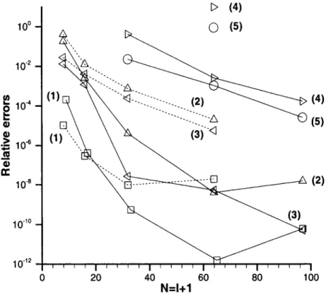
The I1, 1, 1) most fundamental eigenmode (figure 3) is numerically known to a high accuracy since the works of Bj~rstad et al. published in [2,3]. The buckling load problem is indeed solved with quadruple precision by a spectral Legendre-Galerkin method, with N going up to 5000. This provides reference data for a first assessment of the accuracy of our results from both solvers. A systematic comparison is thus performed using the available data, 'namely, the eigenvalue, and the main features of the eigenmode, that is the two leading comer eddies that our solvers are able to resolve. The eddies are characterized by the extremal values of the stream function, (lPext.1 , ~ext,2), and the distance from the comer, (dl, d2), where these values are. Relative errors defined by IX - Xref/Xref] are computed, X standing for the aforementioned quantities, and Xref being taken from [3]. Figure 2 gathers all the relative errors as a function of N --- I + 1. Solid and dashed curves respectively correspond to the PrDi and RH solvers. These curves are numbered (1) for the eigenvalue, (2) and (3) for lPext. I and dl, and (4) and (5) for lPext,2 and d2.

(10)

10 ~ -

1 0 .2 -

~ 10 "4

0

9 ~

lO-e

".~

10 .8

1 0 "10 1 0 "12

(1)1_:.1,

~

'

(1)\~

i i i i i 0

D (4)

9 (5)

" - .

14)

(S)

~ . _ _ _ . _ . _ - - - ~

(2)

20

40

60

80

100

N=I+I

Figure 2. Relative errors I(X - Xref)/Xrefl regarding the I1, 1, 1) most fundamental mode. Solid and

dashed curves respectively correspond to the PrDi and RH solvers. The quantity X successively stands for the eigenvalue (curves (1)), the extremal value of the stream function of the first comer eddy, ~ext, 1 (curves (2)), the location d 1 of this value from the corner, (curves (3)), the extremal value of the stream function of the second comer eddy, ~ext,2 (curves (4)), and the location d 2 of this value from the comer

(curves (5)). Xre f is taken from [3].

Table 1

The fundamental modes eigenvalues: for N = 96 the PrDi absolute eigenvalue Ikl of each symmetry family;

for N = I + 1 = 8, 16, 32, 64 the relative error I(k96 - ~.N)/~.961.

N Scheme [1, 1, 1) I 1 , - 1 , 1) tl, l , - 1 ) t l , - 1 , - 1 ) I - I , / , l) 96 PrDi 13.086172791 38.531365767 8 PrDi 2.14. 10 - 4 1.51 - 10 - 2 RH 1.06.10 - 5 6 . 2 2 . 1 0 - 5 16 PrDi 4 . 0 8 - 1 0 - 7 3 . 8 9 . 1 0 - 8 RH 2 . 9 5 . 1 0 - 7 1.73.10 - 6 32 PrDi 4.90- 10 -10 9.62. 10 -12 RH 9.61 9 10 - 9 4.6. 10 - 8 64 PrDi 6 . 2 4 . 1 0 -11 1.32.10 -11 RH 1.92.10 - 8 3.12- 10 - 9 67.280247001 5.18- 10 - 2 6 . 7 8 . 1 0 - 5 7 . 6 6 . 1 0 - 7 2.41 9 10 - 6 1.95.10 -11 1.16.10 - 7 1 . 8 . 1 0 - 1 ! 4 . 0 8 . 1 0 - 8 32.052396078 6.67- 10 - 4 1.88.10 - 5 6 . 3 3 . 1 0 - 8 5 . 3 2 . 1 0 - 7 9.84 10 - l l 2.28 10 - 7 1.61 10 -11 2.55 10 - 7 23.031098494 3 . 6 7 . 1 0 - 2 1.93.10 - 5 1 . 3 . 1 0 - 7 2 . 2 2 . 1 0 - 7 1.04.10 -10 4.21 9 10 - 7 4 . 3 7 . 1 0 - l l 4 . 4 2 . 1 0 - 7

(11)

E. Leriche, G. Labrosse / Fundamental Stokes eigenmodes in the square 1 2 1 -0 995' ' ' ' ~ o ~ s .... - o ~ " -0 75 -0 8 "0 85 -0 9 - 0 9 5 - - - 5

(b)

X

(a)

' LOESS

(c)

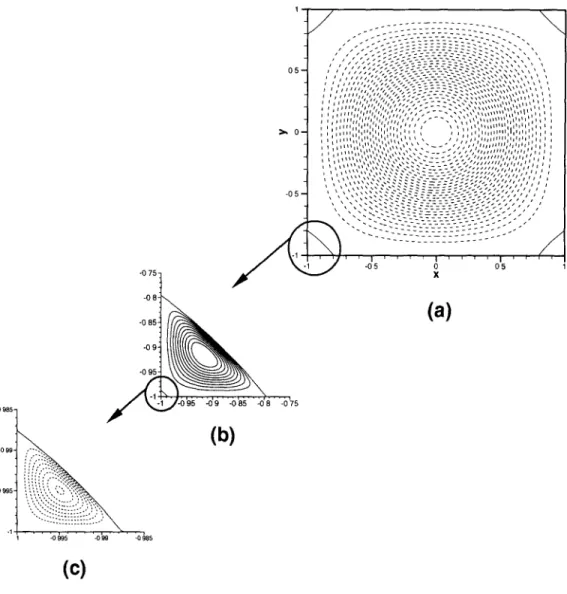
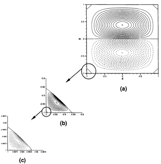
Figure 3. The I1, 1, 1) fundamental mode obtained with the N = 96 Chebyshev solver. Contours of streamlines. (a) Core vortex: minimun contour level -1; maximum level 0; interval of 6.6666 - 1 0 - 2 .

(b) Zoomed primary corner eddy: minimun contour level 0: maximum level -t-1.0 - 1 0 - 4 ; interval of

1.0.10 -5. (c) Zoomed secondary comer eddy: minimun contour level -4.0 - 1 0 - 9 ; maximum level 0;

interval of 4.0 9 10 - 10.

The overall converging behaviour is clear, faster for the eigenvalue computation (curves (1)), and almost systematically better for the PrDi than for the RH solvers. A numerical saturation of the errors on the eigenvalue occurs for N between 64 and 96 for the PrDi solver, and for smaller values of I with the RH solver. Therefore, the RH solver should not be applied with I larger than 63, a cut-off which merely allows to roughly predict the occurence of the second comer eddy (isolated points (4) and (5) in figure 2).

Moreover, the N = 96 PrDi results can be taken as reference data for this work, in absence of any other available published reference data.

(12)

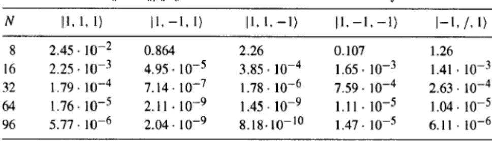
Table 2

The relative norm IIV - ull/llult for the fundamental modes obtained by the PrDi solver.

N I1, 1, 1) I 1 , - l , 1) I1, 1 , - 1 ) I 1 . - 1 , - 1 ) I - 1 , / , 1) 8 2 . 4 5 . 1 0 - 2 0.864 2.26 0.107 1.26 16 2 . 2 5 . 1 0 - 3 4 . 9 5 . 1 0 - 5 3 . 8 5 . 1 0 - 4 1.65- 10 - 3 1.41 9 10 - 3 32 1 . 7 9 . 1 0 - 4 7.14- 10 - 7 1 . 7 8 . 1 0 - 6 7 . 5 9 . 1 0 - 4 2 . 6 3 . 1 0 - 4 64 1 . 7 6 . 1 0 - 5 2.11 9 10 - 9 1 . 4 5 . 1 0 - 9 1.11 9 10 - 5 1 . 0 4 . 1 0 - 5 96 5 . 7 7 . 1 0 - 6 2.04- 10 - 9 8.18.10 - 1 0 1 . 4 7 . 1 0 - 5 6.11 - 10 - 6 5.2. The eigenvalues

Table 1 supplies (a) the absolute eigenvalue I)~961 of each symmetry family fundamental mode, obtained by the N = 96 PrDi solver, followed by (b) the relative error on all other eigenvalues ~.S, measured with the ratio [(~-96 - - ~ N ) / ~ ' 9 6 ] 9

This table indicates that the numerical accuracy supplied by our Chebyshev Stokes solver starts to saturate (for this mode) at about N = 64. The convergence of the eigenvalues coming from the RH expansions is seen to be slower and to saturate at error levels significantly higher than those of the Chebyshev solver.

This shows that enforcing the velocity numerical divergence to be zero can be not better than adequately monitoring its departure from zero, which one decreases exponentially with N (see table 2).

5.3. The eigenmodes

Both schemes are now compared for their ability to provide the main features of the fundamental mode of each symmetry family.

Table 2 reports for these modes the relative norm of V 9 u defined by the ratio

IIV 9 ull/llull, where II,tll stands for the pointwise maximum absolute value of &, and

Ilull = max (llull, Ilvll). The announced exponential decrease with N of this ratio is observed. The main contribution to this ratio comes from the comer eddies. This ratio is thus significantly smaller for the odd comer eddies, those of the I 1, - 1, 1 ) and [ 1, 1, - 1) families, than for the others.

Tables and figures 3-7 provide the results for the fundamental modes by increas- ing value of their IZl. The figures show the stream function contours which come from the almost solenoidal velocity fields supplied by the N = 96 Chebyshev Stokes solver. Each figure presents the core pattern (a), and the primary and secondary comer eddies in successive zooms, (b) and (c), respectively. The data given in the tables are referred to by (a), (b) and (c). For each eigenmode are successively given in the tables, (1) for N = 96, the position of its absolute ~p-extremum (amplitude normalized at 1), and then the position and amplitude of the comer eddies, followed by (2) the corresponding relative errors defined by the ratios [(X96 - XN)/X961, X standing for any of the mentioned quantities obtained at a given N. The stream function extrema are the zeroes of both velocity components. They are computed by applying a Newton-Raphson procedure.

(13)

E. Leriche, G. Labrosse / Fundamental Stokes eigenmodes in the square 123 Table 3

Data regarding the fundamental mode 11, 1, 1): for N = 96, the distance from the corner and amplitude o f the corner eddies, and for N = 1 + 1 = 8, 16, 32, 64 the corresponding relative errors, for the p r o j e c t i o n -

diffusion and R e i d - H a r r i s schemes.

N S c h e m e Primary corner eddy (b) Secondary corner eddy (c)

distance amplitude distance amplitude

96 PrDi 0.118724516366 1.1705464033-10 - 4 7.18776730077- 10 - 3 3.2635770411.10 - 9 8 PrDi 1.32. 10 - 2 0.18 - - RH 0.028 0.41 - - 16 PrDi 1.23- 10 - 3 2 . 6 4 . 10 - 3 - - RH 4.1 - 10 - 3 1 . 2 7 . 1 0 - 2 - - 32 PrDi 2 . 6 7 - 10 - 8 4 . 0 2 - 10 - 6 2 . 2 5 . l0 - 2 0.41 RH 2 . 4 8 . 1 0 - 4 7 . 6 . 1 0 - 4 - - 64 PrDi 5 . 2 8 . 10 - 9 1.94. 10 - 8 1 . 0 7 . 1 0 - 3 2 . 4 7 . 1 0 - 3 RH 5 . 6 3 . 1 0 - 6 2 . 0 4 . 1 0 - 5 0.94 1.0

Often there are several identical (by symmetry) extrema (in the core pattern, and in the corners). Their average positions and amplitudes are then quoted in the forthcoming tables. These tables show that the Chebyshev solver is significantly more efficient for numerically resolving the comer eddies. Indeed, its near boundary spatial resolution in- creases quadratically with N while the Reid-Harris expansion wavenumbers, ~, and ~',, increase only linearly with i.

The fundamental mode I1, 1, 1) (figure 3) is made of only one cell centered at x = y = 0 (x --- 2.0104 9 10 -11, y = 1.1109 9 10 -l~ from the N = 96 Stokes solver), the other extrema being all associated with the corner eddies and lying on the square diagonals. Table 3 gives their amplitude and the distance from the corner where they are located. The Chebyshev solver captures two corner eddies, with a good accuracy with N = 64, whereas the Reid-Harris expansion with the same number of unknowns provides a very rough approximation (amplitude of 4.6 9 1 0 - 1 6 instead of 3 9 1 0 - 9 ) of

the secondary corner eddy, located at a distance of 3.9 9 10 - 4 instead of 7 9 10 -3. For reaching an equivalent accuracy to that of the Chebyshev expansion would require about 300 terms in the Reid-Harris expansion.

The fundamental mode 1 - 1 , / , 1 ) (figure 4) is made of two counter rotating cells located on each side of the horizontal axis ex. The mode I - 1 , / , - 1 ) - not shown - whose eigenvalue is identical, is obtained by a (7r/2)-rotation. The reference extremum of I - 1 , / , 1) is at x = 0 (x = - 8 . 1 7 0 6 . 1 0 -11 from the N = 96 Chebyshev solver) and y given in table 4. The corner eddies have no symmetry about the square diagonals but their symmetrical parts are dominant, explaining the almost equality between the coordinates x and y of the extrema. The average values quoted in the table correspond to the location they have in the top fight corner. The I = 31, 63 Reid-Harris expansions provide very bad approximations of the secondary corner eddy, supplying amplitudes of order 10 - 2 6 instead of 2.10 -9 and distances from the corner of about 2.10 -v instead of 4.10 -3.

(14)

124 E. Leriche, G. Labrosse / Fundamental Stokes eigenmodes in the square -0 9a75 - - 0 9 9 -0 99"25 -0 995 -0 g975 - 1 -0 85 -0 9

(b)

/ \ 0 5 ~ , 0

(a)

(c)

Figure 4. The I - 1 , / , 1) fundamental mode obtained with the N = 96 Chebyshev solver. Contours of streamlines. (a) Core vortex: minimun contour level - 1; maximum level + 1; interval of 6.6666 9 10 - 2 .

(b) Z o o m e d primary comer eddy: minimun contour level 0; maximum level + 9 . 0 9 10-5; interval of 9.0. 10 - 6 . (c) Zoomed secondary comer eddy: minimun contour level - 3 . 0 9 10-9; maximum level 0;

interval of 3 . 0 . 1 0 -10.

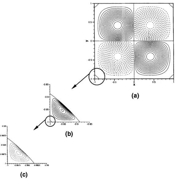
The fundamental mode I 1, - 1, - 1) is shown in figure 5. It is made of four counter rotating cells, located in the sectors made by the axes ex and ~y. It has four identical absolute extrema, of unit amplitude, on the straight lines of equation Ixl = lYl. Their average distance from x = y = 0 is given in table 5. Its comer eddies are symmetrical about the square diagonals, and their average distance from the comer is also reported. Here again, the I = 31, 63 Reid-Harris expansions provide very bad approximations of the secondary comer eddy, supplying amplitudes of order 10 -26 and distances from the comer of about 2 . 1 0 - 7 .

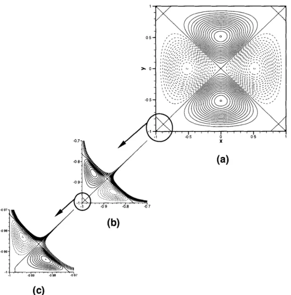
The mode [ 1 , - 1 , 1) (figure 6) is odd under the reflection symmetry about the square diagonals. It has four identical absolute extrema, of unit amplitude, located on

(15)

E. Leriche, G9 Labrosse / Fundamental Stokes eigenmodes in the square 125 Table 4

Data regarding the fundamental mode l - I , / , l ): for N = 96, the position of the core absolute ~ - e x t r e m u m (amplitude normalized at 1), the distance from the comer and amplitude of the comer eddies, and for N = I + 1 = 8, 16, 32, 64 the corresponding relative errors, for the projection-diffusion and Reid-Harris

schemes.

N Scheme Core (a) Primary comer eddy (b) Secondary corner eddy (c)

y x amplitude x amplitude Y 3' 96 PrDi 8 PrDi 0.32 RH 1.28. 10 - 4 1.51 1 . 6 8 16 PrDi 1.59- 10 - 8 2.67 2.34 RH 3 . 9 5 . 1 0 - 6 1.13 5.83 32 PrDi 6 . 7 . 1 0 - l ~ 2.43 1.11 RH 6.51. 10 - 7 1.05 7.71 64 PrDi 1.63. 10 - 9 3.64 3.65 RH 5.59. 10 - 8 7.7- 6.18 • 0.94150948819 8.1764160235.10 - 5 0.99647590506 2.2770846033.10 - 9 0.94203498742 9 1 0 . 2 2 6 . 9 1 0 - 2 . 1 0 - 4 1.46 9 10 - 2 10-6 10 - 3 12. 10-4 10 - 6 1 . 4 7 . 1 0 - 5 10-6 10 - 4 5.5 10-5 10 - 8 6. I 9 10 - 7 10-8 10 - 6 0.21 9 10 - 6 0.99647588429 3.74. 10 - 4 2.32 10 - 4 1. 1. 8.09 10 - 6 5.95 10 - 6 1. 1. 0.356 1. 1.68 9 10 - 2 1. Table 5

Data regarding the fundamental mode I 1 , - 1 , - 1 ) : for N = 96, the position of the core absolute

~ - e x t r e m u m (amplitude normalized at I), the distance from the corner and amplitude of the corner eddies, and for N = I + 1 = 8, 16, 32, 64 the corresponding relative errors, for the projection~liffusion and

Reid-Harris schemes.

N Scheme Core (a) Primary corner eddy (b) Secondary corner eddy (c)

distance distance amplitude distance amplitude

96 PrDi 8 PrDi 5 . 1 6 . 1 0 - 4 RH 2.38. 10 - 5 16 PrDi 6.65- 10 - 8 RH 6.27. 10 - 7 32 PrDi 1.49. 10 - 9 RH 1.71. 10 - 7 64 PrDi 1 . 9 4 . 1 0 -11 RH 9.24- 10 - 8 0.58260184571 0.06576790813 9.1851486567.10 - 5 3.9807584035.10 - 3 2.5552859449.10 - 9 w 6.t I - 10 -1 9.64- 10 - 4 6.22 10 - 3 2.57 10 - 5 6.09 10 - 4 6 . 9 . 1 0 - 8 2 . 7 3 . 1 0 - 4 2.27. 10 - 2 - - 1.86. 10 -1 - - 2,56. 10 - 4 7.57- 10 - 2 1.65 8.89. 10 - 3 1. 1. 1.54. 10 - 8 5.2. 10 - 5 1.24. 10 - I 1.61. 10 - 6 1. 1.

(16)

126 E. Leriche, G. Labrosse / Fundamental Stokes eigenmodes in the square -0 99" -0 9925" "0 995" -0 9 9 7 5 -1 0 5 - 0 9 -0 95

(b)

/ ,,; ,;-::-'_-_--'--.,'- - , , ?;:' IS," ' '""?,"'?'"'i ' ' - 0 5 ,

(c)

Figure 5. The I1, - 1 , - 1 ) fundamental mode obtained with the N = 96 Chebyshev solver. Contours of streamlines. (a) Core vortex: minimun contour level - 1; maximum level + 1; interval of 6.6666 9 10 - 2 . (b) Zoomed primary comer eddy: minimun contour level 0; maximum level 1.0.10-4; interval of 1.0.10 - 5 . (c) Zoomed secondary corner eddy: minimun contour level - 4 . 0 9 10-9; maximum level 0; interval of

4 . 0 . 1 0 - 1 ~

the axes ex and

ey, at

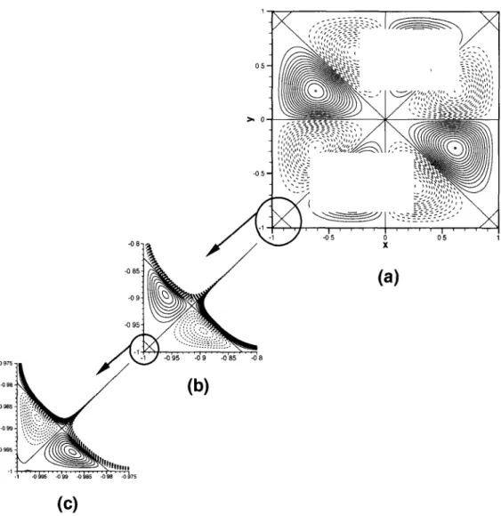
an average distance from x = 0 = y given in table 6. Both coordinates of the comer eddies maxima are also supplied. They do not lie at rr/8 from the square border. Embryonic secondary comer eddies appear in a contour plot of the I = 63 Reid-Harris stream function. Their existence is not quoted in table 6.

At last, the mode I1, 1, - 1) (figure 7), also odd under the reflection symmetry about the square diagonals, is made of eight counter rotating cells, housed by pair in the sectors made by the axes ex and ~ . Its eight identical absolute extrema, of unit amplitude, are at the same distance from x = 0 = y. Their average coordinates are given in table 7, con-

(17)

E. Leriche, G. Labrosse / Fundamental Stokes eigenmodes in the square 127 0 5 84 -0 5

J

~ -0 5 0 ~ . 7 -14 / ]( -0 8

(a)

0 5 1 -0 9 -0 9 -0.8 -0 7

(b)

-1 -099 4) 98 -097

(c)

Figure 6. The I1, - 1 , l) fundamental mode obtained with the N = 96 Chebyshev solver. Contours of streamlines. (a) Core vortex: minimun contour level - 1: maximum level +1; interval of 6.6666 9 10 -2. (b) Zoomed primary comer eddy: minimun contour level - 2 . 0 - 10-5; maximum level 2.0- 10-5; interval of 2.0 9 10 -6. (c) Zoomed secondary comer eddy: minimun contour level - 7 . 0 9 10-11; maximum level

7 . 0 . 1 0 - 1 l ; interval of 7 . 0 . 1 0 -12.

verted for corresponding to the upper rightmost maximum. Both coordinates of the up- per rightmost comer eddy maxima located above the square diagonal are also supplied. With this eigenmode, no comer eddy is captured by the I ~< 63 Reid-Hams expansions.

6. Conclusions

Two spectral expansions are used to compute the Stokes fundamental eigenval- ues and eigenmodes in the square, one for each symmetry family. Firstly, a consistent

(18)

128 E. Leriche, G. Labrosse / Fundamental Stokes eigenmodes in the square

Table 6

Data regarding the fundamental mode I 1, - 1, 1): for N = 96, the position of the core absolute ~p-extremum (amplitude normalized at 1), the distance from the comer and amplitude of the comer eddies, and for

N = I + 1 = 8, 16, 32, 64 the corresponding relative errors, for the projection-diffusion and Reid-Harris

schemes.

N Scheme Core (a) Primary comer eddy (b) Secondary comer eddy (b) distance x amplitude x amplitude

Y Y 96 PrDi 0.51590285446 0,85591228142 1.5762941409.10 - 5 0.98303645693 6.3090863633.10 -11 0,94700951603 0.99379719736 8 PrDi 1.71 9 10 - 2 RH 2 . 0 4 . 1 0 - 4 16 PrDi 3 . 9 2 . 1 0 - 7 RH 5 . 8 9 . 1 0 - 6 32 PrDi 9.27. 10 -12 RH 3.65- t0 - 7 64 PrDi 5 . 3 6 . 1 0 -12 RH 4 . 2 6 . 1 0 - 8 m m 5.77 10 - 7 2.39 10 - 5 3.05 10 - 7 1 . 8 8 - 1 0 - 7 1.75. 10 - 9 1.25. 10 - 9 0.16 5.07. 10 - 2 m 9.02. 10 - 4 4 . 0 3 . 1 0 - 9 1.7. 10 - 3 1.15 9 10 - 3 2 . 9 4 . 1 0 - 8 1 . 5 2 . 1 0 - 7 1 . 6 7 . 1 0 - 7 I . 7 . 2 4 . 1 0 - 2 1.14. l 0 - 4

primitive variables Stokes Chebyshev collocation solver is applied, providing numerical velocities asymptotically divergence free as the discretization is refined. The second ap- proach calls for the Reid-Harris functions for solving the stream function biharmonic problem. A systematic comparison of both schemes with the same number of unknowns is made, its results being reported here. It is clearly stated that the Chebyshev approx- imations are, by far, much more accurate. This is related to their intrinsic high near boundary spatial resolution, improving quadratically with N instead of linearly with the Reid-Harris functions. Moreover this brings a quantitative argument to support the idea that enforcing the solutions to be divergence free is not a guarantee to get them more accurately.

Acknowledgements

The authors would like to thank Prof. M.O. Deville for helpful discussions. The second author gratefully acknowledges the financial support from the ERCOFTAC vis- itor programme sponsored by the L. Euler Pilot Center (Switzerland) at EPFL, and the

(19)

E. Leriche, G. Labrosse / Fundamental Stokes eigenmodes in tile square 129 O- -0 85 -0 5 9 ,-~-~ , "~,, / -os

(a)

0 5 1 -0 95 -0 95 -0 9 -0 85 -0 8

(b)

(c)

Figure 7. The I1, 1 , - 1 ) fundamental mode obtained with the N = 96 Chebyshev solver. Contours of streamlines. (a) Core vortex: minimun contour level - 1 ; maximum level -t-1; interval of 6.6666 - 10 -2. (b) Zoomed primary corner eddy: minimun contour level - 2 . 0 . 10-5; maximum level 2.0- 10-5: interval of 2.0 9 10 - 6 . (C) Zoomed secondary corner eddy: minimun contour level - 7 . 0 - 1 0 - 1 1 ; maximum level

7.0.10-11; interval of 7.0. 10 - 1 2 .

F S T I - E P F L f o r the Invited P r o f e s s o r Fellowship. T h e c o m p u t i n g r e s o u r c e s w e r e m a d e available by C S C S , M a n n o , Switzerland.

References

[1] M. Azaiez, C. Bernardi and M. Grundmann, Spectral method applied to porous media equations, East-West J. Numer. Math. 2 (1995) 91-105.

[2] P.E. BjOrstad and B.P. Tjcstheim, Efficient algorithms for solving a fourth-order equation with the spectral-Galerkin method, SIAM J. Sci. Comput. 18(2) (1997) 621-632.

(20)

Table 7

Data regarding the fundamental mode I 1, 1, - 1 ): for N = 96, the position of the core absolute ~-extremum (amplitude normalized at 1), the distance from the corner and amplitude of the comer eddies, and for N = 1 + 1 = 8, 16, 32, 64 the corresponding relative errors, for the projection--diffusion and Reid-Harris

schemes.

N Scheme Core (a) Primary corner eddy (b) Secondary comer eddy (c)

x x amplitude x amplitude Y Y Y 96 PrDi 0.61492560417 0.89431272505 1.4475288977.10 - 5 0.9875599612 5.7836563585.10 -11 0.26557842863 0.96114272368 0.99545350911 8 PrDi 5 . 5 7 . 1 0 - 3 . . . . 1.33.10 - 2 - RH 2.06- 10 - 4 . . . . 6 . 9 8 . 1 0 - 4 - 16 PrDi 1 . 7 . 1 0 - 6 1.01.10 - 3 6 . 1 6 . 1 0 - 2 - - 1.05- 10 - 5 4 . 4 2 . 1 0 - 4 RH 6 . 2 2 . 1 0 - 6 . . . . 3 . 7 6 . 1 0 - 5 - 32 PrDi 1.75-10 -11 7 . 9 1 - 1 0 - 8 2 . 1 8 . 1 0 - 6 2 . 9 5 . 1 0 - 3 0.41 7 . 9 3 . 1 0 -12 2 . 4 8 . 1 0 - 7 1.27.10 - 3 RH 1.1 - 10 - 7 . . . . 6 . 3 . 1 0 - 7 - 64 PrDi 1.78- 10 -12 3.5- 10 - 9 8 . 0 8 . 1 0 - 8 3 . 7 4 . 1 0 - 6 2 . 1 6 . 1 0 - 4 3 . 1 4 . 1 0 -12 2 . 6 6 . 1 0 - 9 2 . 0 3 . 1 0 - 6 RH 2 . 8 8 . 1 0 - 8 . . . . 1.71 - 10 - 7 -

[3] EE. Bj0rstad and B.P. Tj0stheim, High precision solutions of two fourth order eigenvalue problems, Computing 63(2) (1999) 97-107.

[4] C. Canuto, M.Y. Hussaini, A. Quarteroni and T.A. Zang, Spectral Methods in Fluid Dynamics,

Springer Series in Computational Physics (Springer, New York, 1988).

[5] H.J.H. Clercx, S.R. Maassen and G.J.E van Heijst, Decaying two-dimensional turbulence in square containers with no-slip or stress-flee boundaries, Phys. Fluids I 1(3) (1999) 611-626.

[6] P. Constantin, C. Foias and O.P. Manley, Effects of the forcing function spectrum on the energy- spectrum in 2-d turbulence, Phys. Fluids 6(1) (1994) 427-429.

[7] P.H. Gaskell, J.L. Summers, H.M. Thompson and M.D. Savage, Creeping flow analyses of free surface cavity flows, Theoret. Comput. Fluids Dynamics 8 (1996) 415-433.

[8] D. Gottlieb and S.A. Orszag, Numerical Analysis of Spectral Methods: Theory and Applications

(SIAM/CBMS, Philadelphia, PA, 1977).

[9] D.L. Harris and W.H. Reid, On orthogonal functions which satisfy four boundary conditions. I. Tables for use in Fourier-type expansions, Astrophys. J. Supp. Ser. 3 (1958) 429-447.

[10] R.B. Lehoucq, D.C. Sorensen and C. Yang, ARPACK Users' Guide (SIAM, Philadelphia, PA, 1998).

[11] E. Leriche and G. Labrosse, High-order direct Stokes solvers with or without temporal splitting: Numerical investigations of their comparative properties, SIAM J. Sci. Comput. 22(4) (2000) 1386-

(21)

E. Leriche, G. Labrosse / Fundamental Stokes eigenmodes in the square 131 [12] E. Leriche and G. Labrosse, Stokes eigenmodes in square domain and the stream function - vorticity

correlation, J. Comput. Phys. 200 (2004) 489-511.

[13] H.K, Moffatt, Viscous and resistive eddies near a sharp corner, J. Fluid Mech. 18 (1964) 1-18. [14] S.A. Orszag, M. Israeli and M. Deville, Boundary conditions for incompressible flows, J. Sci. Comput.

1(l) (1986) 75-111.

[15] W.H. Reid and D.L. Harris, On orthogonal functions which satisfy tour boundary conditions. II. Inte- grals for use with Fourier-type expansions, Astrophys. J. Supp. Ser. 3 (1958) 448-452.

[16] I.H. Shames and C.L. Dym, Energy and Finite Element Methods in Structural Mechanics (McGraw- Hill, New York, 1985).

[17] P.N. Shankar, The eddy structure in Stokes flow in a cavity, J. Fluid Mech. 250 (1993) 371-383. [18] J. Sivardiere, La Symetrie en Mathematique, Physique et Chimie (Presses Universitaires de Grenoble,

Grenoble, 1995).

[19] R.C.T. Smith, The bending of a semi-infinite strip, Austral. J. Sci. Res. 5 (1952) 227-237.

[20] L. Sturges and D.D. Joseph, The free surface on a simple fluid between cylinders undergoing torsional oscillations. Part III: Oscillating planes, Archive Rational Mech. Anal. 64 (1977) 245-267.

[21] G.I. Taylor, The buckling load for a rectangular plate with four clamped edges, Z. Angew. Math. Mech. 13(2)(1933) 147-152.

[22] J.A. van de Konijnenberg, J.B. Flor and G.J.E van Heijst, Decaying quasi-two-dimensional viscous flow on a square domain, Phys. Fluids 10(3) (1998) 595-606.

[23] S. Wolframm, Mathematica. A System for Doing Mathematics by Computer (Addison-Wesley, New York, 2000).