HAL Id: hal-01690222
https://hal.archives-ouvertes.fr/hal-01690222v4
Submitted on 29 Mar 2019
HAL is a multi-disciplinary open access
archive for the deposit and dissemination of
sci-entific research documents, whether they are
pub-lished or not. The documents may come from
teaching and research institutions in France or
abroad, or from public or private research centers.
L’archive ouverte pluridisciplinaire HAL, est
destinée au dépôt et à la diffusion de documents
scientifiques de niveau recherche, publiés ou non,
émanant des établissements d’enseignement et de
recherche français ou étrangers, des laboratoires
publics ou privés.
Distributed under a Creative Commons Attribution - NonCommercial - NoDerivatives| 4.0
International License
and locally irregular decompositions
Olivier Baudon, Julien Bensmail, Tom Davot, Hervé Hocquard, Jakub
Przybylo, Mohammed Senhaji, Eric Sopena, Mariusz Woźniak
To cite this version:
Olivier Baudon, Julien Bensmail, Tom Davot, Hervé Hocquard, Jakub Przybylo, et al.. A general
decomposition theory for the 1-2-3 Conjecture and locally irregular decompositions. Discrete
Mathe-matics and Theoretical Computer Science, DMTCS, 2019, ICGT 2018, 21 (1). �hal-01690222v4�
A general decomposition theory for the 1-2-3
Conjecture and locally irregular
decompositions
∗
Olivier Baudon
1Julien Bensmail
2Tom Davot
3Hervé Hocquard
1Jakub Przybyło
4Mohammed Senhaji
1Éric Sopena
1Mariusz Wo´zniak
41
LaBRI, Université de Bordeaux, France
2
I3S/INRIA, Université Nice-Sophia-Antipolis, France
3
Université de Montpellier, CNRS, LIRMM, France
4
AGH University of Science and Technology, al. A. Mickiewicza 30, 30-059 Krakow, Poland
received 13thJuly 2018, revised 1stMar. 2019, accepted 25thMar. 2019.
How can one distinguish the adjacent vertices of a graph through an edge-weighting? In the last decades, this question has been attracting increasing attention, which resulted in the active field of distinguishing labellings.
One of its most popular problems is the one where neighbours must be distinguishable via their incident sums of weights. An edge-weighting verifying this is said neighbour-sum-distinguishing. The popularity of this notion arises from two reasons. A first one is that designing a neighbour-sum-distinguishing edge-weighting showed up to be equivalent to turning a simple graph into a locally irregular (i.e., without neighbours with the same degree) multigraph by adding parallel edges, which is motivated by the concept of irregularity in graphs. Another source of popularity is probably the influence of the famous 1-2-3 Conjecture, which claims that such weightings with weights in {1, 2, 3} exist for graphs with no isolated edge.
The 1-2-3 Conjecture has recently been investigated from a decompositional angle, via so-called locally irregular de-compositions, which are edge-partitions into locally irregular subgraphs. Through several recent studies, it was shown that this concept is quite related to the 1-2-3 Conjecture. However, the full connexion between all those concepts was not clear.
In this work, we propose an approach that generalizes all concepts above, involving coloured weights and sums. As a consequence, we get another interpretation of several existing results related to the 1-2-3 Conjecture. We also come up with new related conjectures, to which we give some support.
Keywords: 1-2-3 Conjecture, Locally irregular decompositions, Coloured weighted degrees
1
Introduction
The current work is mainly related to the well-known 1-2-3 Conjecture, which is defined accordingly to the upcoming notions. Let G be a graph, and let ω be an edge-weighting (assigning weights among {1, . . . , k}) of G. From ω, one can design the vertex-colouring σ of G where each vertex v gets assigned, as its colour σ(v), the sum of weights (called its weighted degree) assigned to its incident edges. That is, for every vertex v of G we have
σ(v) := X
u∈N (v)
ω(uv),
where N (v) denotes the set of neighbours of v. In case σ is actually a proper vertex-colouring of G, i.e., we have σ(u) 6= σ(v) for every two adjacent vertices u and v, then we call ω neighbour-sum-distinguishing.
∗This work was partly conducted during the Master internship of the third author, done at LaBRI under the supervision of the first
and seventh authors. The second author’s research was supported by PEPS grant POCODIS. The fifth author’s research was supported by the National Science Centre, Poland, grant no. 2014/13/B/ST1/01855. The fifth and eighth authors’ research was partially supported by the Faculty of Applied Mathematics AGH UST statutory tasks within subsidy of Ministry of Science and Higher Education.
For any two graphs G and H, we say that G has no isolated H if no connected component of G is isomorphic to H. Note that all graphs with no isolated edge admit neighbour-sum-distinguishing edge-weightings (consider e.g. an inductive argument). Graphs with no such connected components are thus called nice, with respect to this edge-weighting notion. The 1-2-3 Conjecture, posed in 2004 by Karo´nski, Łuczak and Thomason [9], asks whether, for every nice graph, we can design neighbour-sum-distinguishing 3-edge-weightings, i.e., using weights 1, 2, 3 only. More precisely, if we denote by χΣ(G) the least k
such that a nice graph G admits a neighbour-sum-distinguishing k-edge-weighting, then it is believed that χΣ(G) ≤ 3 should always hold.
1-2-3 Conjecture (Karo´nski, Łuczak, Thomason [9]). For every nice graph G, we have χΣ(G) ≤ 3.
Despite many active investigations in the last decade, the 1-2-3 Conjecture is still wide open to date. These investigations have been mainly focused on 1) proving the 1-2-3 Conjecture for new classes of nice graphs, 2) proving general constant upper bounds on χΣ, and 3) studying side aspects of the 1-2-3 Conjecture. As
the literature on this topic is vast, a brief summary of some of these investigations is deferred to the next section.
The current work is also related to locally irregular decompositions, which were considered as a de-compositional approach towards understanding some aspects behind the 1-2-3 Conjecture. In general, by a decomposition of a graph, we mean an edge-colouring where each colour class yields a graph with par-ticular properties. A locally irregular graph is a graph in which every two adjacent vertices have distinct degrees. By a locally irregular decomposition of a graph, we thus mean a decomposition into locally irreg-ular graphs. Sticking to the edge-colouring point of view, we will also sometimes instead speak of a locally irregular edge-colouring.
Locally irregular decompositions relate to the 1-2-3 Conjecture through, notably, the following argu-ments. In a sense, the graphs G that are the “most convenient” for the 1-2-3 Conjecture are those which verify χΣ(G) = 1. Those graphs are precisely the locally irregular ones. Also, in particular contexts,
locally irregular decompositions can be turned into neighbour-sum-distinguishing edge-weightings. Per-haps the best illustration of that claim is the fact that, in any regular graph, a neighbour-sum-distinguishing 2-edge-weighting yields a decomposition into two locally irregular graphs, and vice versa.
Similarly as for neighbour-sum-distinguishing edge-weightings, there exist graphs which do not admit any locally irregular decomposition; but, this time, the class of exceptional graphs is much wider (consider e.g. any path of odd length). An exceptional graph (with respect to locally irregular decompositions) is also called an exception, for short. Conversely, a graph that is not exceptional is said decomposable. For a decomposable graph G, we denote by χ0irr(G) the least k such that G admits a locally irregular k-edge-colouring. Similarly as in the case of the 1-2-3 Conjecture, it is believed that every decomposable graph should decompose into at most three locally irregular graphs, as conjectured by some of the authors of the present paper:
Conjecture 1.1 (Baudon, Bensmail, Przybyło, Wo´zniak [3]). For every decomposable graph G, we have χ0
irr(G) ≤ 3.
Conjecture 1.1 was first verified for a few graph classes. Also, general constant upper bounds on χ0irrwere recently exhibited. For the sake of keeping the introduction short, we again refer the reader to the next section for a survey of some of these results.
In this work, we aim at introducing a general decompositional theory enclosing neighbour-sum-distinguishing edge-weightings and locally irregular decompositions. This theory is mainly based on the observation that a locally irregular `-edge-colouring of a graph G is, put differently, a decomposition of G into graphs G1, . . . , G`verifying χΣ(G1), . . . , χΣ(G`) = 1. This leads us to combine the notions of
neighbour-sum-distinguishing edge-weightings and locally irregular edge-colourings, in the following way. Let `, k ≥ 1 be two integers, and G be a graph. To each edge of G, we assign, via a colouring ω, a pair (α, β), where α ∈ {1, . . . , `} and β ∈ {1, . . . , k}, which can be regarded as a coloured weight (with value β and colour α). Now, for every vertex v of G, and every colour α ∈ {1, . . . , `}, one can compute the weighted α-degree σα(v), being the sum of weights with colour α incident to v. So, to every vertex v is associated a palette
(σ1(v), . . . , σ`(v)) of ` coloured weighted degrees.
When working on variants of the 1-2-3 Conjecture, the intent is to design edge-weightings ω that allow to distinguish the adjacent vertices, accordingly to some distinction condition. When dealing with the notions introduced in the last paragraph, there are many ways for asking for distinction, as several coloured sums
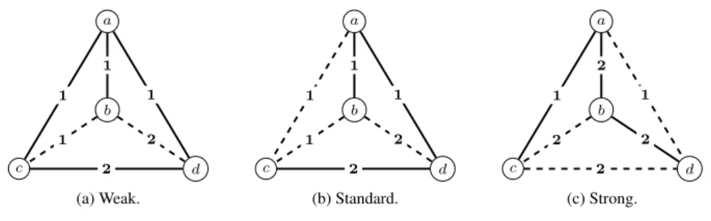
a b c d 1 1 1 1 2 2 (a) Weak. a b c d 1 1 1 1 2 2 (b) Standard. a b c d 1 2 2 1 2 2 (c) Strong. Figure 1: Three (2, 2)-colourings of K4.
are available; in this work, we will focus on the following three distinction variants, which sound the most natural to us:
• Weak distinction: two adjacent vertices u and v of G are considered distinguished if there is an α ∈ {1, . . . , `} such that σα(u) 6= σα(v).
• Standard distinction: two adjacent vertices u and v of G are considered distinguished if, assuming ω(uv) = (α, β), we have σα(u) 6= σα(v).
• Strong distinction: two adjacent vertices u and v of G are considered distinguished if, for every α ∈ {1, . . . , `}, we have σα(u) = σα(v) = 0, or σα(u) 6= σα(v).
Assuming ω verifies one of the weak, standard or strong distinction condition for every pair of adjacent vertices, we say that ω is a weak, standard or strong (`, k)-edge-colouring, and that G is weakly, standardly or strongly (`, k)-coloured. We also say that G is weakly, standardly or strongly (`, k)-colourable, if there are `0, k0 ≥ 1 with `0 ≤ ` and k0 ≤ k such that G can be weakly, standardly or strongly (`0, k0)-coloured,
respectively.
We provide, in Figure 1, an illustration of these concepts on K4, the complete graph on four vertices,
where the two colours are represented by solid and dashed edges. By the “incident solid sum” of a vertex, we here mean the sum of weights assigned to its incident solid edges. It can be checked that, in Figure 1.(a), the depicted (2, 2)-colouring is a weak colouring. It is however not a standard (2, 2)-colouring as vertices c and d are joined by a solid edge but their incident solid sums equal 3. The colouring in Figure 1.(b) is a standard (2, 2)-colouring which is not a strong colouring, in particular because vertices a and c both have incident solid sum 2. The colouring in Figure 1.(c) is a strong (2, 2)-colouring.
This paper is organized as follows. As already mentioned, the notions of weak, standard and strong (`, k)-colourings can be employed to generalize neighbour-sum-distinguishing edge-weightings and locally irregular edge-colourings. In Section 2, we explore these connexions. In particular, we recall known results and translate them in our new terminology.
Playing with the parameters ` and k and the distinction conditions, we also come up with new problems, some of which we believe are of independent interest. In particular, we wonder whether almost all graphs can be weakly, standardly, or even strongly (2, 2)-coloured. If true, this would imply side decomposition results related to the 1-2-3 Conjecture. The strong, standard and weak versions of that question are formally introduced in Section 3. They are then studied in Sections 4, 5 and 6, respectively.
2
Previous results and connexions to (`, k)-colourings
As a warm up, we start, in Section 2.1, by making first observations and remarks on weak, standard and strong colourings. We then survey, in Section 2.2, some of the results from literature that are directly connected to these notions. More precisely, we explain which notions in the literature are encompassed by weak, standard and strong colourings, and, by rephrasing known results under that new terminology, we exhibit first results.
2.1
Early observations
First of all, we note that, according to the definitions, every result holding for some version of (`, k)-colourings also holds for the weaker versions. This is why, throughout Sections 4 to 6, we start by consid-ering strong colourings, then standard colourings, and, finally, weak colourings.
Observation 2.1. A strong (`, k)-colouring is also a standard (`, k)-colouring. Analogously, a standard (`, k)-colouring is also a weak (`, k)-colouring.
In general, though, it can be observed that the converse direction is not true, i.e., that a given (`, k)-colouring does not necessarily fulfil stronger distinction conditions. A good illustration for that is the fact that K3 can be weakly (2, 2)-coloured but not standardly (2, 2)-coloured. There are situations, though,
where all distinction conditions behave similarly. We state a few of them below.
First of all, we recall that, for some values of ` and k, some versions of (`, k)-colourings are equivalent to other kinds of distinguishing colourings and weightings. Most of these observations are straightforward, and thus do not need a formal proof. In particular, it can easily be checked that some of these results do not hold for stronger or weaker versions of our colouring variants.
Observation 2.2. Weak, standard and strong (1, k)-colourings and neighbour-sum-distinguishing k-edge-weightings are equivalent notions.
Observation 2.3. Standard (k, 1)-colourings and locally irregular k-edge-colourings are equivalent no-tions.
Let G be a graph, and ω be an edge-weighting of G. For each vertex v of G, one can compute its multisetµ(v) of incident weights induced by ω. We say that ω is neighbour-multiset-distinguishing if no two adjacent vertices of G get the same multiset of incident weights. Note that having σ(u) 6= σ(v) for an edge uv of G implies that µ(u) 6= µ(v) (but the converse is not necessarily true). For this reason, neighbour-multiset-distinguishing edge-weightings have been studied as a weaker form of neighbour-sum-distinguishing edge-weightings.
The point for mentioning neighbour-multiset-distinguishing edge-weightings is that they relate to our notion of weak colourings.
Observation 2.4. Weak (k, 1)-colourings and neighbour-multiset-distinguishing k-edge-weightings are equivalent notions.
In Observation 2.2, we noticed that, for (1, k)-colourings, all three distinction conditions are equivalent. In the following result, we point out another context where the three colouring variants coincide.
Observation 2.5. In regular graphs, weak, standard and strong (2, 1)-colourings are equivalent notions.
2.2
Previous results
In this section, we restate, in our terminology, several results from the literature on distinguishing weightings and colourings to derive the existence of particular (1, k)- or (`, 1)-colourings. In other words, we here point out how our colouring concepts encapsulate existing distinguishing weightings and colourings.
This section is not intended to be a full survey on variants of the 1-2-3 Conjecture. Hence, we voluntarily focus on those existing results that are closely related to our investigations; for more details, please refer to the survey [12] by Seamone.
2.2.1
Neighbour-sum-distinguishing edge-weightings
Recall that, according to Observation 2.2, being strongly (1, k)-colourable is equivalent to being neighbour-sum-distinguishing k-edge-weightable. Thus, all general constant upper bounds on χΣ yield results on
strong colourability (hence on the weaker variants as well, recall Observation 2.1).
In the context of neighbour-sum-distinguishing edge-weightings, the leading conjecture is the 1-2-3 Con-jecture. If true, that conjecture would imply that every nice graph is strongly (1, 3)-colourable. Recall that nice graphs are exactly those graphs without isolated edges.
Conjecture 2.6. Every nice graph is strongly (1, 3)-colourable.
To date, the best result towards the 1-2-3 Conjecture was given by Kalkowski, Karo´nski and Pfender [8], who proved χΣ(G) ≤ 5 for every nice graph G. As said above, this result can be stated as follows, using
our terminology.
Theorem 2.7. Every nice graph is strongly (1, 5)-colourable.
The 1-2-3 Conjecture was shown to hold for several common classes of nice graphs, such as complete graphs and 3-colourable graphs. There exist graphs G verifying χΣ(G) = 3, such as complete graphs of
settled the question in the negative [6], by showing that determining the exact value of χΣ(G) is an
NP-complete problem. Later on, Ahadi, Dehghan and Sadeghi [2] proved that this remains true when restricted to regular (cubic) graphs. This result is of prime interest, as all distinguishing weighing and colouring notions considered in this paper tend to be equivalent when 1) only two weights or colours are considered, and 2) the graph is regular (recall Observation 2.5). This result, by itself, directly establishes the general hardness of weak, standard and strong colourings.
It took some time to settle this complexity question for bipartite graphs. In a first work [7], Chang, Lu, Wu and Yu provided several sufficient conditions for a nice bipartite graph G to verify χΣ(G) ≤ 2.
In particular, they showed that being connected and having one of the two partite sets of even cardinality is a sufficient condition, and, from this result, they easily proved that nice trees always admit neighbour-sum-distinguishing 2-edge-weightings. Later on, the full characterization of connected bipartite graphs G with χΣ(G) = 3 was given by Thomassen, Wu and Zhang [13], who proved that they are exactly the
odd multicacti. These graphs can be constructed as follows. Start from m ≥ 1 cycles C1, . . . , Cmwhose
lengths are at least 6 and congruent to 2 modulo 4, and colour the edges of the Ci’s using colours red and
green alternately. Then, an odd multicactus is any connected graph obtained from the Ci’s via repeated
applications of the following operation: pick two connected components G1and G2, and identify a green
edge of G1with a green edge of G2. Said differently, an odd multicactus is obtained by identifying edges
of particular cycles in a tree-like fashion. In particular, every cycle with length congruent to 2 modulo 4 is an odd multicactus.
Theorem 2.8 (Thomassen, Wu, Zhang [13]). A connected bipartite graph G verifies χΣ(G) = 3 if and
only ifG is an odd multicactus.
2.2.2
Locally irregular edge-colourings
By Observation 2.3, we get that locally irregular k-edge-colourings are precisely standard (k, 1)-colourings. We thus survey some of the research on locally irregular edge-colourings, as they transfer to standard (k, 1)-colourings.
As mentioned in Section 1, not all graphs decompose into locally irregular graphs, so one has to deal with so-called exceptions. In their first work on this topic [3], Baudon, Bensmail, Przybyło and Wo´zniak completely characterized all connected exceptions. Namely, connected exceptions include 1) odd-length paths, 2) odd-length cycles, and 3) the family T defined recursively as follows:
• The triangle K3belongs to T.
• Every other graph in T can be constructed by 1) taking an auxiliary graph F being either a path of even length or a path of odd length with a triangle glued to one of its ends, then 2) choosing a graph G ∈ T containing a triangle with at least one vertex, say v, of degree 2 in G, and finally 3) identifying v with a vertex of degree 1 of F .
Note that all connected exceptions have maximum degree at most 3.
Thus, a graph is decomposable if and only if it has no exception as a connected component. Once the set of exceptions was characterized, Baudon, Bensmail, Przybyło and Wo´zniak conjectured that every decomposable graph G should decompose into at most three locally irregular graphs, i.e., χ0irr(G) ≤ 3. Due to Observation 2.3, this conjecture can be restated as follows:
Conjecture 2.9. Every decomposable graph is standardly (3, 1)-colourable.
The first constant upper bound on χ0irris due to Bensmail, Merker and Thomassen [5], who proved that we have χ0irr(G) ≤ 328 for every decomposable graph G. This bound was recently improved down to 220 by Lužar, Przybyło and Soták [10]. We can thus state the following:
Theorem 2.10. Every decomposable graph is standardly (220, 1)-colourable.
Baudon, Bensmail, Przybyło and Wo´zniak verified Conjecture 2.9 for several decomposable graph classes [3], including complete graphs, some bipartite graphs, some Cartesian products, and regular graphs with degree at least 107. Later on, Przybyło [11] verified the conjecture for graphs with minimum degree at least 1010. The complexity aspects were considered by Baudon, Bensmail and Sopena [4], who proved that, for a given graph G, deciding whether χ0irr(G) = 2 is NP-complete in general, while determining χ0irr(G) can be done
2.2.3
Neighbour-multiset-distinguishing edge-weightings
As mentioned in the previous section, all sum-distinguishing edge-weightings are neighbour-multiset-distinguishing, but the converse is not always true. The connexion between these two notions was first considered by Karo´nski, Łuczak and Thomason in the paper introducing the 1-2-3 Conjecture [9]. The first formal study of neighbour-multiset-distinguishing edge-weightings may be attributed to Addario-Berry, Aldred, Dalal and Reed, who, later on, gave improved results towards a “multiset version” of the 1-2-3 Conjecture [1]. In our terminology, this conjecture reads as follows:
Conjecture 2.11. Every nice graph is weakly (3, 1)-colourable.
So far, the best result towards Conjecture 2.11 is hence due to Addario-Berry, Aldred, Dalal and Reed, who proved that all nice graphs admit neighbour-multiset-distinguishing 4-edge-weightings [1].
Theorem 2.12. Every nice graph is weakly (4, 1)-colourable.
All graph classes verifying the 1-2-3 Conjecture also verify Conjecture 2.11. Additionally, the latter conjecture was also verified for graphs with minimum degree at least 1000, see [1].
3
New problems
As seen in Section 2, some of the (1, k)-colouring and (`, 1)-colouring variants correspond to distinguishing weighting and colouring notions already considered in the literature. In particular, for such values of ` and k, there is still some gap between the corresponding conjectures and the best results we know to date. One way to get some sort of side progress, could be to prove the existence of (`, k)-colourings (for some distinction condition) where ` + k or max{`, k} is as small as possible.
In particular, the main problem we consider in the rest of this paper, which corresponds to minimizing max{`, k}, and to which we could not find any obvious counterexample, reads as follows. By a nicer graph, we mean a graph with no isolated edges and triangles.
Conjecture 3.1. Every nicer graph is strongly (2, 2)-colourable.
The main reason for suspecting that K2and K3might be the only connected graphs admitting no strong
(2, 2)-colourings is that they are the only connected exceptional graphs (recall the exact characterization in Subsection 2.2.2) admitting no neighbour-sum-distinguishing 2-edge-weightings.
Observation 3.2. Every connected exception different from K2andK3verifies Conjecture 3.1.
Proof: Let G be a connected exception different from K2and K3. We consider several cases corresponding
to the three families of connected exceptions given by the definition:
• If G is an odd-length path, then G is a connected bipartite graph different from an odd multicactus, thus verifies χΣ(G) ≤ 2 according to Theorem 2.8, and hence admits strong (1, 2)-colourings.
• If G is an odd-length cycle with length at least 5, then G can be decomposed into two paths Pr, Pb
with length at least 2. In particular, the end-vertices of Pr(and similarly Pb) are not adjacent in G,
and we have χΣ(Pr), χΣ(Pb) ≤ 2. By considering a strong (1, 2)-colouring of Pr(with red weights)
and a strong (1, 2)-colouring of Pb(with blue weights), we eventually get a strong (2, 2)-colouring
of G.
• Finally assume that G ∈ T \ {K3}. By contracting the triangles (there is at least one such) of G to
vertices, we obtain a tree R(G) with maximum degree 3, whose some nodes (triangle nodes) corre-spond to triangles of G, while some nodes (normal nodes) correcorre-spond to real vertices. Furthermore, by definition, any path of R(G) joining two triangle nodes has odd length, and any path joining a triangle node and a pendant normal node has even length.
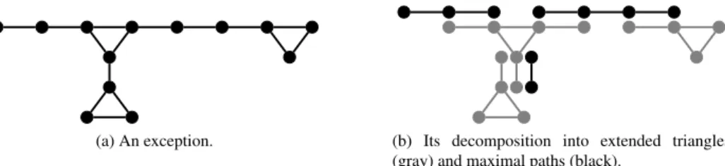
We can consider G as a collection of triangles with at most three pendant edges attached (extended triangles), and paths with one or two ends attached to a triangle (maximal paths) (see Figure 2 for an example). The pendant edges attached to the extended triangles, as well as the end-edges incident to triangles of the maximal paths, are called attachment edges. According to these definitions, G can be constructed from extended triangles and maximal paths by glueing their attachment edges. In particular, every attachment edge belongs to one extended triangle and one maximal path.
(a) An exception. (b) Its decomposition into extended triangles (gray) and maximal paths (black).
Figure 2: Decomposing an exception as described in the proof of Observation 3.2.
Necessarily R(G) has a degree-1 node r, being either a triangle node (pendant triangle in G) or a normal node (pendant vertex in G). Consider the (virtual) orientation of the edges of R(G) from r towards the leaves. We construct a strong (2, 2)-colouring (assigning weights coloured red and blue) iteratively, by extending a colouring along extended triangles and maximal paths following the ordering given by the orientation of the attachment edges. Since R(G) is a tree, note that once an attachment edge is coloured, this provides a pre-colouring of the next extended triangle or maximal path to be coloured.
We start constructing the colouring from r. In G, node r corresponds either to an end-vertex of a maximal path P (normal node), or to a triangle T (triangle node). In the first case, let P := v1. . . v2k;
then we just assign red weights 1, 2, 2, 1, 1, . . . along P . In the second case, let T := v1v2v3v1, and
let v10 denote, without loss of generality, the neighbour of v1outside T ; we here assign red weight 1
to v3v2and red weight 2 to v2v1, and blue weight 1 to v3v1and blue weight 2 to v1v10. In any case, it
can be checked that the colouring is correct so far.
We now proceed to the general case, i.e., we consider a maximal path P or extended triangle T whose one attachment edge is coloured, and we extend the colouring to all its other attachment edges in G. Consider first a maximal path P := v1. . . vk whose attachment edge v1v2was assigned, say, a red
weight. We here extend the colouring to all edges of P by assigning red weights (with value 1 or 2) to its edges v2v3, . . . , vk−1vksuccessively. Note that this can be done correctly, as, when a red weight
is being assigned to an edge vivi+1, we just have to make sure that the red sum of viavoids the red
sum of vi−1, which is possible since we have two red weights to play with.
We are left with the case where the colouring must be extended to an extended triangle T := v1v2v3v1
whose one attachment edge, say v1v10, was previously assigned, say, a red weight. We here consider
cases depending on the number of additional attachment edges:
– If v1v01is the only attachment edge of T , then we assign a red weight to v1v2so that the red sum
of v1does not get equal to the red sum of v01. We then assign blue weights 1, 2 or 2, 1 to v1v3
and v3v2in such a way that the blue sum of v1does not get equal to the blue sum of v10.
– Assume v2v20 is the only other attachment edge of T . We here assign a red weight to v1v3in
such a way that the red sum of v1does not get equal to the red sum of v10. We then assign blue
weights 1, 2, 1 or 2, 1, 1 to v2v1, v2v3and v2v02in such a way that the blue sum of v1does not
get equal to the blue sum of v10.
– Lastly, assume v2v02 and v3v03 are attachment edges. First, we assign blue weight 1 to v1v2
and blue weight 2 to v1v3. We now assign red weight 1 to v02v2, red weight α to v2v3and red
weight 2 to v3v30, where α is the red weight of v10v1.
In any of these cases, it can be checked that the colouring extension is correct. So this covers all cases of the proof.
The rest of this paper is dedicated to providing evidences towards Conjecture 3.1. We do it gradually, by first considering, in Section 4, Conjecture 3.1 in its literal form. We then consider its standard version (in Section 5), before finally considering its weak version (in Section 6).
4
Strong (`, k)-colouring
Strong Conjecture. Every nicer graph is strongly (2, 2)-colourable.
We verify the Strong Conjecture for nicer complete graphs and bipartite graphs. Recall that every result on strong (2, 2)-colourings directly transfers to standard and weak (2, 2)-colourings.
We start off with complete graphs. For every n ≥ 1, we denote by Knthe complete graph with order n.
Theorem 4.1. For every n ≥ 4, the graph Knis strongly(2, 2)-colourable.
Proof: We prove the claim by induction on n. To ease the proof, we prove a stronger statement, namely that every complete graph Kn admits a strong (2, 2)-colouring with red and blue weights such that either
there is no vertex incident to red edges only, or there is no vertex incident to blue edges only.
As a base step, consider K = K4. Note that K can be decomposed into two paths Prand Pbof length 3.
To get a strong (2, 2)-colouring, we proceed as follows (see Figure 1.(c), where Pr, Pb are the paths with
solid and dashed edges, respectively). Consider first the edges of Prfrom one end to the other, and assign
them red weights 1, 2, 2, respectively. Similarly, then consider the edges of Pbfrom one end to the other,
and assign them blue weights 1, 2, 2, respectively. Since Prand Pbspan all vertices of K, each vertex gets
a non-zero red sum and a non-zero blue sum. This, by itself, guarantees that the additional requirement is fulfilled (i.e., there is no monochromatic vertex). Now, due to how the red weights were assigned, it can easily be seen that the obtained red sums are 1, 2, 3, 4; hence no two vertices get the same red sums. As this is also the case for the blue sums, we have thus constructed a strong (2, 2)-colouring of K.
We now prove the general case. Let K = Kn(where n ≥ 5), and remove one vertex v from K. We end
up with a graph isomorphic to Kn−1, which, by the induction hypothesis, admits a strong (2, 2)-colouring
with colours red and blue. Furthermore, we may, without loss of generality, assume that, by this colouring, there is no vertex incident to red edges only. We extend this colouring to K, i.e., to the edges incident to v, by assigning red weight 2 to all those edges. As a result, all red sums of the vertices of V (K) \ {v} rise by 2, and since every two of them were different, they still are after the extension. Now, note that the red sum of v is precisely 2(n − 1), which is strictly greater than all the other red sums since all vertices of V (K) \ {v} are incident to blue edges. Furthermore, the blue sums of the vertices of V (K) \ {v} have not been altered, while v has blue sum 0 – so no two non-zero blue sums are the same. We thus get a strong (2, 2)-colouring of K, and it can be noted that no vertex is incident to blue edges only, as additionally required.
We now prove the Strong Conjecture for bipartite graphs. Recall that a connected bipartite graph G verifies χΣ(G) = 3 if and only if it is an odd multicactus (Theorem 2.8).
Theorem 4.2. Every nice bipartite graph G is strongly (2, 2)-colourable.
Proof: We can assume that G is connected. If G is not an odd multicactus, then χΣ(G) ≤ 2, and,
equiva-lently, G is strongly (1, 2)-colourable. So let us now assume that G is an odd multicactus. By construction, note that G necessarily has a degree-2 vertex v. Furthermore, G is 2-connected, so the graph G0:= G − {v} is connected. Also, G0 is not an odd multicactus (to be convinced of this, note that it has degree-1 vertices and that one of its partite sets if of even cardinality). So G0is strongly (1, 2)-colourable.
Consider thus a strong (1, 2)-colouring of G0assigning red weights. We extend this colouring to a strong (2, 2)-colouring of G, i.e., to the edges u1v and vu2incident to v, by just assigning blue weights 1 and 2
to u1v and vu2, respectively. As no new edge was assigned a red weight, the adjacent red sums are still
different in G. Also, v has red degree 0. Furthermore, the only three non-zero blue sums are all different, as they are equal to 1, 2 and 3.
In the rest of this section, we confirm that odd multicacti are a peculiar class of nice bipartite graphs for the distinguishing colouring notions we consider, in the following sense.
Theorem 4.3. A connected nice bipartite graph cannot be strongly (2, 2)-coloured if and only if it is an odd multicactus.
The proof of Theorem 4.3 relies on the following result on locally irregular decompositions of odd mul-ticacti, which we believe is of independent interest, as there is still no known characterization of bipartite graphs G verifying χ0irr(G) ≤ 2.
Lemma 4.4. For every odd multicactus G, we have χ0irr(G) = 3.
Proof: Let G be an odd multicactus. As such (recall the description in Subsection 2.2.1), G has edges coloured red and green “alternatively”. To avoid any confusion with the colours, in the rest of the proof we refer to the green edges of G as its attachment edges, while we refer to the red edges as its support edges.
Since G is an odd multicactus, by construction there has to be an attachment edge uv such that u and v are joined by several disjoint non-trivial paths P1, . . . , Pk of length congruent to 1 modulo 4, whose
removal does not disconnect the graph. In some sense, the Pi’s are leaves in the tree representation of the
construction of G. Along such a path Pi, if wx and yz are two edges at distance 2 (thus xy is an edge, and
x, y have degree 2), then wx and yz must have different colours in any locally irregular 2-edge-colouring of G, as otherwise x and y would be adjacent and have the same degree in the subgraph induced by the colour assigned to xy. Since every Pihas length congruent to 1 modulo 4, this means that, in every locally
irregular 2-edge-colouring of G, the first and last edges of each Pimust be assigned a same colour. Thus,
from the point of view of uv, colouring the Pi’s is similar to colouring k parallel edges joining uv. Said
differently, if the multigraph G0, obtained by replacing the Pi’s by k parallel (attachment) edges joining
u and v, admits no locally irregular 2-edge-colouring, so neither does G. This operation, consisting in contracting non-trivial paths joining a “leaf” attachment edge, is called a contraction below.
By repeatedly applying contractions (note that the argument above works even if the non-trivial paths have parallel attachment edges), we get a series of multigraphs G = G0, G1, . . . , Gm= G0such that 1) if
Gi+1admits no locally irregular 2-edge-colourings, then so does not Gi, and 2) G0consists of two vertices
joined by several parallel (attachment) edges. Since G0 admits no locally irregular 2-edge-colouring (its two vertices are necessarily adjacent and have the same degree in every colour assigned to some edges), this gives the conclusion for G.
We can now prove Theorem 4.3:
Proof of Theorem 4.3: Let G be a connected nice bipartite graph. If G is not an odd multicactus, then χΣ(G) ≤ 2 (Theorem 2.8), and hence G is strongly (1, 2)-colourable. So we may assume that G is an
odd multicactus, and thus that G is not strongly (1, 2)-colourable. In that case, according to Lemma 4.4, G admits no locally irregular 2-edge-colourings, hence no strong (2, 1)-colourings.
5
Standard (`, k)-colouring
We here consider the standard weakening of Conjecture 3.1:
Standard Conjecture. Every nicer graph is standardly (2, 2)-colourable.
Note that a standard (`, k)-colouring is nothing but a decomposition into ` graphs admitting neighbour-sum-distinguishing k-edge-weightings. From that perspective, it could be interesting to wonder whether graphs, in general, decompose into a constant number of graphs verifying the 1-2-3 Conjecture. We believe this is an interesting aspect to consider, as not many graphs are known to verify the 1-2-3 Conjecture.
Towards the Standard Conjecture, we thus also raise the following related conjecture, which is, in a sense, a weakening of the 1-2-3 Conjecture:
Conjecture 5.1. Every nice graph is standardly (2, 3)-colourable. That is, every nice graph decomposes into two graphs verifying the 1-2-3 Conjecture.
In this section, towards the Standard Conjecture, we first improve Theorem 2.10 by showing that all nice graphs admit standard (40, 3)-colourings. We then prove the Standard Conjecture 5.1 for nicer 2-degenerate graphs and subcubic graphs, before proving Conjecture 5.1 for nice 9-colourable graphs.
5.1
Standard (40, 3)-colourability
The proof of the following result follows the lines of one in [5], where Bensmail, Merker and Thomassen proved that decomposable graphs can be decomposed into at most 328 locally irregular graphs.
Theorem 5.2. Every decomposable graph G is standardly (40, 3)-colourable.
Proof: In G, we can find a locally irregular subgraph H1such that G − E(H1) has all of its connected
components being of even size ([5], Lemma 2.1). If G already had even size, then H1is empty. Still calling
G the remaining graph, we can decompose G into a graph H2 with minimum degree at least 1010 and a
(2 · 1010+ 2)-degenerate graph H
3whose all connected components are of even size ([5], Lemma 4.5).
On the one hand, according to a result of Przybyło [11], we can decompose H2into three (possibly empty)
locally irregular graphs H2,1, H2,2, H2,3. On the other hand, H3can be decomposed into 36 bipartite graphs
Recall that every locally irregular graph H verifies χΣ(H) = 1. Furthermore, all nice bipartite graphs
verify the 1-2-3 Conjecture. From these arguments, using a set of 40 coloured weights 1, 2, 3 to indepen-dently weight the edges of each of the Hi’s and the Hi,j’s, we eventually get a standard (40, 3)-colouring
of G.
Since all connected nice exceptional graphs are 3-colourable, they verify the 1-2-3 Conjecture (see [12]), and are thus standardly (1, 3)-colourable. Together with Theorem 5.2, this yields the following:
Theorem 5.3. Every nice graph G is standardly (40, 3)-colourable.
5.2
The Standard Conjecture for 2-degenerate graphs and subcubic graphs
Recall that a graph is 2-degenerate if every of its subgraphs has a vertex with degree at most 2. A subcubic graphis a graph G with maximum degree at most 3. If all vertices of G have degree precisely 3, then we call G cubic. Furthermore, if G is connected and not cubic, i.e., G has vertices with degree 1 or 2, then we say that G is strictly subcubic.
We first prove the Standard Conjecture for 2-degenerate graphs (with a few exceptions). More precisely, we prove:
Theorem 5.4. Every nicer 2-degenerate graph G is standardly (2, 2)-colourable.
Our proof of Theorem 5.4 relies on the following lemma, which is proved later in this section. Lemma 5.5. Every nicer 2-degenerate graph G decomposes into two nice forests.
Proof of Theorem 5.4: According to Lemma 5.5, we can decompose G into two forests Frand Fb none
of which has an isolated edge. Since every nice tree T verifies χΣ(T ) ≤ 2 (i.e., admits standard (1,
2)-colourings), each of Frand Fb, independently, admits a standard (1, 2)-colouring; let ωrand ωbbe any such
for Frand Fb, respectively. To get a standard (2, 2)-colouring of G, we consider all weights assigned by ωr
and ωb, and colour red those weights originating from ωr, while we colour blue those weights originating
from ωb.
We are left with proving Lemma 5.5.
Proof of Lemma 5.5: Throughout the proof, which is by induction on |V (G)| + |E(G)|, we assume that G is connected. As a base case, it can be checked that the claim is true whenever |V (G)| ≤ 4. In particular, under all conditions, G is either 1) a nice tree (in which case the claim holds trivially), 2) a triangle with a pendant vertex attached (which decomposes into two paths of length 2), 3) two triangles glued along an edge (which decomposes into a path of length 2 and a star with three leaves), or 4) a cycle of length 4 (which decomposes into two paths of length 2).
Let us thus proceed to the proof of the general case (in particular, |V (G)| ≥ 5). First assume that G has a degree-1 vertex v. Denote by u the neighbour of v in G, and let G0:= G − {v}. Since |V (G)| ≥ 5, note that G0 cannot be K2or K3. So, by the induction hypothesis, G0 decomposes into a red nice forest and a
blue nice forest. Assuming u belongs to the red forest, we extend that decomposition to G by adding vu to the red forest.
Thus, we may assume that G has a degree-2 vertex v, with neighbours u1, u2. We distinguish two cases:
• First case: v is a cut-vertex. Let H1and H2be the two connected components of G − {v}, where
uibelongs to Hifor i = 1, 2, and set G1:= H1+ {u1v} and G2:= H2+ {u2v}. Since G has no
degree-1 vertex, note that none of G1and G2is isomorphic to K2. Also, v has degree 1 in both G1and
G2, so none of G1and G2is isomorphic to K3. By the induction hypothesis, G1and G2decompose
into two nice forests. Note that these two decompositions, when combined in G, altogether form a decomposition of G into two nice forests.
• Second case: v is not a cut-vertex. Note that G0 := G − {v} is nicer, as it is a connected graph
with |V (G0)| ≥ 4. By the induction hypothesis, G0 thus decomposes into two nice forests, say red and blue. If u1 belongs to the blue forest while u2 belongs to the red forest, then we extend this
decomposition to G by assigning colour blue to vu1and colour red to vu2. So we may assume that
u1does not belong to the blue forest, in which case we extend the decomposition to G by assigning
colour blue to both vu1, vu2. This way, either a pendant path of length 2 is attached to a blue tree
(if u2belongs to the blue forest), or a path of length 2 is added to the blue forest (otherwise). As all
This concludes the proof.
We now extend the previous results to nicer subcubic graphs.
Lemma 5.6. Every nicer subcubic graph G decomposes into two nice forests.
Proof: Throughout the proof, which is by induction on |V (G)| + |E(G)|, it is assumed that G is con-nected. As the claim is true whenever |V (G)| ≤ 4 (G is either strictly subcubic and the result follows from Lemma 5.5, or isomorphic to K4, which decomposes into two paths of length 3), we proceed to the proof
of the general case.
We now consider the general case |V (G)| ≥ 5. If G is strictly subcubic, then G is 2-degenerate, in which case the result follows from Lemma 5.5. So let us assume that G is cubic. Let v be a (degree-3) vertex of G, with neighbours u1, u2, u3. Note that if all edges among the ui’s exist, then G is K4while |V (G)| ≥ 5,
a contradiction. Hence, assume without loss of generality that u1u2is not an edge of G. Consider the graph
G0:= G − {v} + {u1u2}. Note that, although G0might consist of up to two connected components, none
of them is isomorphic to K2 or K3 as G is cubic. So all connected components are subcubic, and they
decompose into two nice forests, say red and blue.
Consider the decomposition of G0. Suppose that u1u2belongs to the red forest. We consider the same
decomposition in G, except that, since G does not contain the edge u1u2, we replace it, in the red forest, by
the two edges u1v and vu2. Note that, in G, the red subgraph remains a nice forest. It thus remains to add
vu3to either the red or blue forest. If u3belongs to the blue forest, then we are done when adding vu3to
the blue forest. So assume that the two edges, different from vu3, incident to u3belong to the red forest. If
v and u3belong to different trees of the red forest, then we can freely add vu3to the red forest. So lastly
suppose that we are not in that case.
All of u1, u2, u3belong to the same tree, say T , of the red forest. In T , let us assume that u3is closer
to u2than it is closer to u1. In other words, in T , the only path from u3to u1passes through u2. Let us
remove vu2from T . In the red forest, T is disconnected into two trees T0 and T00, where T0 contains u2
and u3, while T00contains v and u1. Note that T0is not isomorphic to K2, since u3remains of degree 2 in
that tree. If T00also has this property, then we get a desired decomposition of G when adding vu2and vu3
to the blue forest (recall that u3originally did not belong to the blue forest). So we may assume that T00is
actually isomorphic to K2, which means that u1had degree 1 in T . In this situation, we obtain the desired
decomposition of G by adding vu1and vu3to the blue forest.
A similar proof as that used to prove Theorem 5.4, but using Lemma 5.6 instead of Lemma 5.5, now yields the following.
Theorem 5.7. Every nicer subcubic graph is standardly (2, 2)-colourable.
5.3
Conjecture 5.1 for 9-colourable graphs
To prove Conjecture 5.1 for all nicer 9-colourable graphs, we essentially prove that 9-colourable graphs, in general, decompose into two nice 3-colourable graphs. With such a result in hand, we can then use the fact that nice 3-colourable graphs verify the 1-2-3 Conjecture.
Lemma 5.8. Assume that a nicer graph G can be 2-edge-coloured with red and blue so that the induced red subgraphGRand blue subgraphGBsatisfyχ(GR) = r and χ(GB) = b with r, b ≥ 2. Then G can be
2-edge-coloured in such a way that χ(GR) ≤ r, χ(GB) ≤ b, and GRandGBare nice.
Proof: Consider a 2-edge-colouring of G with red and blue yielding a red subgraph GRand a blue subgraph
GB. Among all possible such colourings, we consider one where χ(GR) ≤ r ≥ 3 and χ(GB) ≤ b ≥ 3
that minimizes the number of monochromatic K2’s. Note that if G has isolated triangles, then, by the latter
requirement, they are monochromatic. Our goal is to show that we can modify the colouring so that the number of monochromatic K2’s is reduced, while retaining the 3-colourability of GR, GB.
Assume uv is isolated in the blue subgraph GB. We note that u, v must belong to the same component
of GR, as otherwise we could just recolour uv red, and get our conclusion (as joining two disjoint
3-colourable graphs via an edge yields a 3-3-colourable graph). Also, if uw is a red edge adjacent to uv, then, when recolouring uw blue, we must create a new isolated edge in the red subgraph, as otherwise our conclusion would be reached (because attaching a pendant path of length 2 to a 3-colourable graph yields a 3-colourable graph). Thus, we may assume that, for every red edge uw (resp. vw), the size of the component of GR− {uw} (resp. GR− {vw}) that contains w is exactly 1.
From the previous arguments, we can deduce that u, v have degree precisely 2 in G, and that the second neighbour of both u, v is a same vertex w. This vertex w cannot have degree 2, as otherwise u, v, w would belong to an isolated triangle of G, which is impossible since all isolated triangles are coloured in a monochromatic way. So w has degree at least 3 in G, and all edges incident to w different from wu, wv are coloured blue. We get here the desired 2-edge-colouring when recolouring wu, wv blue (as attaching a triangle onto a vertex of a 3-colourable graph yields a 3-colourable graph).
We now prove the second key lemma of this section.
Lemma 5.9. Every 9-colourable graph G decomposes into an r-colourable graph GRand ab-colourable
graphGBwithr, b ≤ 3.
Proof: Let G be a graph with χ(G) ≤ 9, and let V0, ..., V8be a proper 9-vertex-colouring of G. We
2-edge-colour G with 2-edge-colours red and blue, yielding two subgraphs GRand GB, respectively, as follows. Consider
any edge uv, where u ∈ Viand v ∈ Vjfor some i 6= j ∈ {0, ..., 8}. We colour uv red if and only if i = j
(mod 3). Otherwise, i.e., when i 6= j (mod 3), we colour uv blue. Now GRis a 3-colourable graph with
proper 3-vertex-colouring V0∪ V1∪ V2, V3∪ V4∪ V5, V6∪ V7∪ V8, while GBis a 3-colourable graph with
proper 3-vertex-colouring V0∪ V3∪ V6, V1∪ V4∪ V7, V2∪ V5∪ V8.
We are now ready to prove that nice 9-colourable graphs verify Conjecture 5.1. Theorem 5.10. Every nice 9-colourable graph G is standardly (2, 3)-colourable.
Proof: If G is 3-colourable, then we have χΣ(G) ≤ 3 (see [9]), or, in other words, G is standardly (1,
3)-colourable. Now assume that G is at least 4-chromatic. By Lemma 5.9, it can be decomposed into two 3-colourable graphs: an r-colourable graph GRand a b-colourable graph GB with r, b ≤ 3. Since G is at
least 4-chromatic we have also r, b ≥ 2. We distinguish two cases:
• If G has no isolated triangles, then, by Lemma 5.8, it can be decomposed into two nice graphs GR
and GBwith χ(GR) ≤ r and χ(GB) ≤ b with r, b ≥ 3. So, both of them verify the 1-2-3 Conjecture,
and thus admit standardly (1, 3)-colourings. Combining standardly (1, 3)-colourings of GRand GB,
we get a standard (2, 3)-colouring of G.
• If G has isolated triangles, then we remove those from G, apply the previous point to get a (2, 3)-colouring of what is left, and then give the same color to all the edges of the isolated triangles. Finally, by weighting the edges of each isolated triangle with weights 1, 2, 3 (in any colour), we can extend the (2, 3)-colouring to G.
This ends up the proof.
We note that the approach above can be generalized to show that, in general, any nice graph G decom-poses into at most blog3χ(G)c + 1 graphs fulfilling the 1-2-3 Conjecture. To see this holds, set k = χ(G)
and consider a proper k-vertex-colouring of G with parts V0, ..., Vk−1. Now, for every i 6= j ∈ {0, ..., k−1},
assuming x ∈ {1, ..., blog3χ(G)c + 1} is the right-most position at which the ternary representations of
i and j differ, we assign colour x to all edges uv of G where u ∈ Vi and v ∈ Vj. It can be observed
that this results in a (blog3χ(G)c + 1)-edge-colouring of G where each colour class yields a 3-colourable
graph. Using Lemma 5.8, we can ensure these 3-colourable graphs are nice, thus that they fulfil the 1-2-3 Conjecture.
6
Weak (`, k)-colouring
We finally consider the weaker form of Conjecture 3.1 (which would follow from the 1-2-3 Conjecture, if it turned out to be proved):
Weak Conjecture. Every nice graph is weakly (2, 2)-colourable.
Towards the Weak Conjecture, we here prove that all nice graphs are weakly (3, 2)- and (2, 3)-colourable. Both proofs are based on the fact that every nice graph admits a neighbour-sum-distinguishing 5-edge-weighing, as proved by Kalkowski, Karo´nski and Pfender [8].
Proof: Slight modifications of the proof of Kalkowski, Karo´nski and Pfender [8] allow to show that every nice graph even admits a neighbour-sum-distinguishing {s − 2, s − 1, s, s + 1, s + 2}-edge-weighting, for any integer s. Let thus ω be a neighbour-sum-distinguishing {−2, −1, 0, 1, 2}-edge-weighting of G. We deduce a weak (3, 2)-colouring of G by modifying and colouring the weights of ω, as follows:
• we colour red every edge with value in {1, 2};
• we colour blue every edge with value in {−2, −1}, and multiply its value by −1; • we colour green every edge with value 0, and change its value to 1.
The key point is that, through ω, every two adjacent vertices u and v are only distinguished via their incident edges with weight in {−2, −1, 1, 2}. Said differently the edges with weight 0 are useless for distinguishing u and v. This implies that, in the obtained (3, 2)-colouring, it is not possible that both the red and blue sums of u and v are equal. From this reasoning, we get that the resulting (3, 2)-colouring is indeed a weak (3, 2)-colouring.
Theorem 6.2. Every nice graph G is weakly (2, 3)-colourable.
Proof: The proof of Kalkowski, Karo´nski and Pfender [8] that every nice graph G admits a sum-distinguishing 5-edge-weighting can be modified to prove that every nice graph admits a neighbour-sum-distinguishing {1, 2, 3, 4, 6}-edge-weighting. We voluntarily do not give the full proof of this claim in details, as the proof would be identical to the original one. Instead, we point out the main differences with the original proof (employing the same terminology as in [8]):
• At the beginning of the algorithm, all edges vivjare assigned weight f (vivj) = 4.
• For every backward edge vjvi(j < i), the possible valid moves are the following:
– If f (vjvi) = 4, then doing either −2 (changing the weight to 2) or +2 (changing the weight to
6) is a valid move, depending on whether the current sum of vj is the biggest or the smallest,
respectively, among its two allowed ones.
– If f (vjvi) = 3, then doing −2 (changing the weight to 1) is a valid move.
– If f (vjvi) = 1, then doing +2 (changing the weight to 3) is a valid move.
• Whenever it is needed to modify the weight f (vivj) of the first forward edge (i < j) incident to vi
in order to define the two allowed sums for vi, doing either −1 (changing the weight to 3) or −3
(changing the weight to 1) to f (vivj) is a valid move. Furthermore, we can choose the two sums
allowed for viand perform valid moves on edges incident to viso that:
– If f (vivj) is changed to 3, then the current sum of viis the biggest of the two allowed ones.
– If f (vivj) is changed to 1, then the current sum of viis the smallest of the two allowed ones.
Let us now prove that if G is a nice graph, then it is weakly (2, 3)-colourable. Let ω be a neighbour-sum-distinguishing {1, 2, 3, 4, 6}-edge-weighting of G. We deduce a weak (2, 3)-colouring of G by 2-colouring and (possibly) altering the weights assigned by ω, as follows:
• we colour red every edge with value in {1, 3};
• we colour blue every edge with value in {2, 4, 6}, and halve its value.
Consider an edge uv of G. Note that if the red sums of u and v are equal, then their blue sums cannot be equal too: in such a situation, we would get σω(u) = σω(v), a contradiction. So we get a weak (2,
3)-colouring.
Acknowledgements
The authors would like to thank anonymous referees for suggesting many valuable improvements to previ-ous versions of the current paper, regarding, notably, Theorems 6.1 and 6.2.
References
[1] L. Addario-Berry, R.E.L. Aldred, K. Dalal, B.A. Reed. Vertex colouring edge partitions. Journal of Combinatorial Theory, Series B, 94(2):237-244, 2005.
[2] A. Ahadi, A. Dehghan, M-R. Sadeghi. Algorithmic complexity of proper labeling problems. Theoret-ical Computer Science, 495:25–36, 2013.
[3] O. Baudon, J. Bensmail, J. Przybyło, M. Wo´zniak. On decomposing regular graphs into locally irreg-ular subgraphs. European Journal of Combinatorics, 49:90-104, 2015.
[4] O. Baudon, J. Bensmail, and É. Sopena. On the complexity of determining the irregular chromatic index of a graph. Journal of Discrete Algorithms, 30:113-127, 2015.
[5] J. Bensmail, M. Merker, C. Thomassen. Decomposing graphs into a constant number of locally irreg-ular subgraphs. European Journal of Combinatorics, 60:124-134, 2017.
[6] A. Dudek, D. Wajc. On the complexity of vertex-coloring edge-weightings. Discrete Mathematics Theoretical Computer Science, 13(3):45-50, 2011.
[7] G.J. Chang, C. Lu, J. Wu, Q. Yu. Vertex-coloring edge-weightings of graphs. Taiwanese Journal of Mathematics, 15(4):1807-1813, 2011.
[8] M. Kalkowski, M. Karo´nski, F. Pfender. Vertex-coloring edge-weightings: towards the 1-2-3 Conjec-ture. Journal of Combinatorial Theory, Series B, 100:347-349, 2010.
[9] M. Karo´nski, T. Łuczak, A. Thomason. Edge weights and vertex colours. Journal of Combinatorial Theory, Series B, 91:151–157, 2004.
[10] B. Lužar, J. Przybyło, R. Soták. New bounds for locally irregular chromatic index of bipartite and subcubic graphs. Preprint arXiv:1611.02341.
[11] J. Przybyło. On decomposing graphs of large minimum degree into locally irregular subgraphs. Elec-tronic Journal of Combinatorics, 23(2):#P2.31, 2016.
[12] B. Seamone. The 1-2-3 Conjecture and related problems: a survey. Technical report, available online at http://arxiv.org/abs/1211.5122, 2012.
[13] C. Thomassen, Y. Wu, C.-Q. Zhang. The 3-flow conjecture, factors modulo k, and the 1-2-3-conjecture. Journal of Combinatorial Theory, Series B, 121:308-325, 2016.