HAL Id: hal-03024749
https://hal.univ-reunion.fr/hal-03024749
Submitted on 26 Nov 2020HAL is a multi-disciplinary open access
archive for the deposit and dissemination of sci-entific research documents, whether they are pub-lished or not. The documents may come from teaching and research institutions in France or abroad, or from public or private research centers.
L’archive ouverte pluridisciplinaire HAL, est destinée au dépôt et à la diffusion de documents scientifiques de niveau recherche, publiés ou non, émanant des établissements d’enseignement et de recherche français ou étrangers, des laboratoires publics ou privés.
Distributed under a Creative Commons Attribution| 4.0 International License
areas of current desertification : a case study in Senegal
Waldir de Carvalho Junior, Maud Loireau, Mireille Fargette, Braz Calderano
Filho, Abdoulaye Wélé
To cite this version:
Waldir de Carvalho Junior, Maud Loireau, Mireille Fargette, Braz Calderano Filho, Abdoulaye Wélé. Correlation between soil erosion and satellite data on areas of current desertification : a case study in Senegal. Ciência e trópico, 2017, Ciência e Trópico, 41 (2), pp.51-66. �hal-03024749�
ERODIBILITY AND SATELLITE DATA ON
AREAS OF CURRENT DESERTIFICATION:
a case study in Senegal
1Waldir de Carvalho Junior2 Maud Loireau3 Mireille Fargette4 Braz Calderano Filho5 Abdoulaye Wélé6
ABSTRACT
The purpose of the study is to verify whether some correlation exists between soil erodibility (i.e. K factor mentioned in RUSLE model) and data obtained from satellite images. This piece of work represents a first attempt towards a model that would predict the risk for soil erosion, from information contained in satellite images. Ouarchoch is a rural community in Ferlo Region, Senegal. It lies in a Sahelian typical arid zone and is affected by desertification processes. Ouarchoch site was the pilot area on which the test was performed. K factor was calculated by using soil textural data (sand, silt and clay) in the top (0 – 5 cm) soil layer (data obtained from the web). Landsat7 satellite images
1 We would like to thank the extra contributors: Sanaa Lakhlifi, Sane Mamadou, Therese Libourel, Cesar da Silva Chagas, Télésphore Brou, Abdoulaye Faye and Samira El Yacoubi.
2 PhD in Soil Science in Universidade Federal de Viçosa (UFV), Brazil, 2005 and Posdoc in digital soil mapping at Institue National de Researche Agricole (INRA), France, 2012. Currently is a Researcher in Brazilian Agricultural Research Corporation. waldir.carvalho@embrapa.br
3 PhD in Geography (Spatial organization: dynamics and Management of rural areas) at University of Montpellier III; member of French scientific committee on desertification (CSFD). maud.loireau@ird.fr
4 PhD in Agronomy Ecole Nationale Supérieure d’Agronomie (Montpellier SupAgro, France); She has been working for Institut de Recherche pour le Développement (IRD). mireille.fargette@ird.fr
5 PhD in Geology from Universidade Federal do Rio de Janeiro (UFRJ), Brasil; 2012; Currently is a researcher in the Brazilian Agricultural Research Corporation. braz.calderano@embrapa.br
6 Engineer of Water and Forests with specialization in ecologist. Currently is a researcher in CSE – Centre de Suive Ecologique – Senegal. wele@cse.en
represented different seasonal snapshots (“cool” dry season, warm dry season, rainy season, end of rainy season or beginning of dry season) of the same year, 2014. Calculation used Bands 1 to 7 and Normalized Difference Vegetation Index (NDVI). The choice of data, calculation and analysis are detailed. Some positive moderate correlation exists between soil erodibility on the one hand, and NDVI index displayed during the dry season (images in January and May), as well as Band 5 radiations displayed at the beginning of the dry season (post-harvest, image in October) on the other hand.
KEYWORDS: Soil erosion risk. Soil erodibility. Socio environmental
correlations. Desertification.
Submission date: 12/04/2017 Acceptance date: 16/06/2017
1 INTRODUCTION
The severe and combined actions of water and wind erosion can contribute to land degradation. They are closely associated to each other both in time and space in sandy areas in Sahel (RAJOT
et al., 2009). Rainfall spans over a rather short period of time (from
June to September). Runoff intensity, in micro-basins, depends on rain intensity, soil physico-chemical characteristics and vegetation cover, and causes loss of soil. Especially during dry seasons, eroded material accumulated in places is taken over by wind and translocated further away. Because of the wind, sandy soils loose the first organo-mineral horizon; the mineral horizon lies exposed and its surface, polished by grains saltation, gets more impermeable and makes rainwater infiltration less easy; this, in turn, promotes water erosion (MAINGUET; DUMAY, 2011). Depending on the depletion and accumulation of material trans-ported by water and/or wind, degraded areas occur when soils (shallow, depleted or gullied…) no longer play their substract role for crops or spontaneous plants.
In this context, soil erosion risk assessment is a complex endeavour because of a number of concurrent processes, either natural (linked or not to climate change) or anthropogenic (linked to soil use and management and various upstream or downstream human activities). This, in turn, affects socio environmental interactions, both in time and space. There
is no current generic model that integrates wind erosion. In contrast, there exists a model for soil erosion risk, as far as water is concerned: the Universal Soil Loss Equation (USLE) (WISCHMEIER; SMITH, 1978) is based on land physical properties and climate features. This universal equation was adapted (equation – RUSLE) by distinguishing five factors: erosivity (R), soil erodibility (K), slope length and steepness (LS), crop management (C), and practice factor (P).
The use of remote sensing and satellite images in order to spatialize / map erosion risk is an area of research which has been explored over the past decade. Indeed, such device should be in position to provide frequent and updated information to stakeholders and environmental risk managers, as soon as one or several factors (among the 5 factors of RUSLE model) would be “related” to satellite images information. For example Al-Abadi et al. (2016), Bahrawi et al. (2016) and Patil et
al. (2015) used Landsat8 or IRS P6 images and NDVI calculation to
estimate C factor (crop management) respectively in Iraq, Saudi Arabia, and India. Wilford et al. (2016) assessed the environmental correlation to establish predictive relationships between geochemical concentration and the environmental covariates. They show that the environmental correlation approach generates high resolution predictive maps that are statistically more accurate and effective than ordinary kriging and inverse distance weighting interpolation methods.
In this work, we chose to focus on soil erodibility (i.e. its resis-tance to rainfall at the surface of the soil, and to runoff notch) because the higher the soil erodibility, the greater the risk of rainfall erosion and further wind erosion. From there, we tackle the overall soil erosion risk and land degradation. From data analysis carried out in different agro ecological situations across Africa, RUSLE model points at the very aggressive rain regime to account for much erosion in Africa. However, soil erodibility is not homogeneous in space and time: it is more acute during rainy seasons and also depends on soil characteristics, age of clearing and cultivation techniques. That being said, studies of erodibility in Africa are very scarce, there are few data, in time and space (ROOSE; DE NONI, 2004).
Indeed, soil erodibility ground data are not easy to collect and a prediction model of soil erodibility, based on data more easily available (satellite images for instance), would be very useful. As mentioned
above for C Factor, previous pieces of work intended to feed RUSLE model with satellite data in order to produce maps on soil erosion risk. The aim of the present work not only points at K Factor, but also tackle the question through the possible correlation between independent sets of data - soil erodibility (K factor) on the one hand and data contained in satellite images on the other hand. A significant correlation would provide a milestone in the attempt to predict soil erodibility; this would further forecast the use of satellite data for soil surveys throughout larger areas.
2 MATERIAL AND METHODS
The approach is tested on a pilot area in a Sahelian typical arid zone affected by desertification processes (2.1). The approach takes into account soil data together with the difficult access to soil erodibility ground data (2.2.) and the variation in space and time contained in satellite data (2.3). The approach verifies the absence of artefact related to sampling design on correlation results (2.4).
2.1 THE STUDY AREA
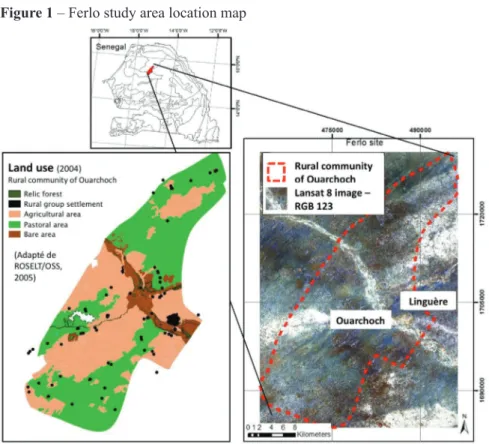
Ouarchoch, a rural community in Ferlo Region, Linguere Department (Figure 1) is located in south of Senegal Basin, in Northern Senegal (from 14,5º to 16,1º N and 12,9º to 16,0º W), and covers an area of approximately 71.000 km2. As a part of the Western Africa shield,
the region is flat and not higher than 70 m, with an average altitude of 40 m above sea level. The region is part of the semi-arid Sahel: annual rainfall of 410.4 mm in average with one rainy season and a long, dry, hot season with temperature ranging from 21.1ºC and 36.1ºC (Figure 2). It is worth noting that in 2014 (when the selected satellite images were collected, cf. 2.3), the amount of rain was lower than average. Soil occupation consists in steppe (50%) dedicated to pastoral use; cropping plots (25%) and fallows (15%) dedicated to agricultural use; bare areas (7%) along the banks of dry riverbeds in valleys, relict forest (2%), rural group settlements and pools (1%) (Figure 1). The vegetation cover never exceeds 20%, except in relict forest where it can reach 60%. Steppe (possibly including trees and/or shrubs) is mostly to be found south and north of the study area.
Soils are mostly tropical ferruginous with little or no leaching, very sandy, fairly degraded, poor in organic matter, low in fertility, very sensitive to erosion. The soil in shallow places and between inter dunes has much finer texture and is fairly covered with relict forest, has a higher fertility but such places are not (or rarely) cultivated. Such soils are more stable and less prone to degradation. Lowland soils lay in between these two types, have intermediate texture, are less prone to erosion, but very poor in organic matter and exchangeable bases (cathions). The soil surface is sandy in most areas and there are particular areas with lateritic profiles.
Figure 1 – Ferlo study area location map
Figure 2 – Monthly rainfall in Linguere Region (red curve: average data between 1960 and 2014;blue curve: data for 2014) (Worldclim)
Source: ANACIM (Agence Nationale de l’Aviation Civile et de la Météorologie, Sénégal).
2.2 K FACTOR
Given the difficulty in collecting sufficient data to adequately measure K Factor, early in the USLE’s history the soil erodibility nomo-graph method was developed to estimate K on the basis of standard soil properties. At the time the nomograph approach was developed, only a small number of soils samples has been collected in the United States; it is hence necessary to check the nomograph’s ability to predict the soil’s true erodibility in other contexts. For example, to determinate K Factor into RUSLE model, Terranova et al. (2009) required data on texture, structure, organic matter, and permeability fixed for each soilscape in soil maps; Prasannakumar et al. (2012) considered the particle size, organic matter content and permeability class.
Considering that data on soil organic matter are difficult to obtain, and because there is little MO quantity in arid zone soils, it would be interesting to base the assessment of soil erodibility factor (K factor) only on soil textural data (BAGARELLO et al., 2012). For example, Xu et al. (2013) already focused on soil texture (data corresponding to fractions of sand, silt and clay). In that study, K Factor used for USLE
(Wischmeier and Smith, 1978) was calculated by only incorporating the soil textural data (sand, silt and clay) of the topsoil (0 – 5 cm layer) into equation developed by Mannigel et al. (2002):
K Factor = ((%sand + %silt)/(%clay))/100
Data on soil properties (sand, silt and clay composition) of topsoil layer (0 – 5 cm) in Africa maps, 250 m resolution, are produced by ISRIC - World Soil Information / AfSIS Project, and available on the web7 (Soil property maps of Africa at 250 m). Such data were produced
by prediction models (random forest and kriging) using MODIS and SRTM by independent variables and the parameters of African soil database by dependant variables. Maps of Senegal has been down-loaded and square covering Ouarchoch community extracted. Due to the pixel size, the images were resampled to 30 m to fit the satellite images resolution.
For this preliminary attempt, we decided to focus on the only (0-5 cm) topsoil layer, which is very sensitive to rainfall erosion. Along the same line, further studies could also include the layer (5-15 cm)8
provided by ISRIC - World Soil Information at least, and even the 6 layers provided (down to 100-200m)9
2.3 SATELLITE IMAGES
Satellite images sensor ETM + Landsat7 images collected on January 30th, May 22nd, August 26th and October 13th 2014 were
avail-able on NASA and USGS websites. January, May, August and October correspond to “cool” dry season, warm dry season, rainy season, end of rainy season or beginning of dry season respectively.
The four images share the same characteristics, as described in
Table 1, with respect to spectral ranges and resolution.
7 http://www.isric.org/data/afsoilgrids250m
8 The first soil horizon in the study area is either absent or does not exceed 15 cm, except in depression areas.
Table 1 – Landsat7 image characteristics
Bands Spatial resolution (m) Spectral range (μm) Common applications B1 30 0.450 to 0.515 (blue-green) Coastal water mapping; differentiation of vegetation from soils B2 30 0.525 to 0.605 (green) Assessment of vegetation vigor B3 30 0.63 to 0.69(red) Chlorophyll absorption for vegetation differentiation B4 30 0.75 to 0.90 (infra-red) Biomass surveys and delineation of water bodies B5 30 (mid-infrared I)1.55 to 1.75 Vegetation and soil moisture measurements; differentiation between snow and cloud B6 60 (thermal infrared)10.4 to 12.50 Thermal mapping, soil moisture studies, Plant heat stress measurement B7 30 (mid-infrared II)2.09 to 2.35 Hydrothermal mapping NDVI 30 (B4-B3)/(B4+B3) Vegetation cover measurements
Source: Landsat 7 handbook - http://landsathandbook.gsfc.nasa.gov/
Since data used for the K factor calculation have a 250 m resolution and because landscapes span over hundreds of hectar in the large area of Ouarchoch rural community, the 30 m resolution of Landsat7 images and their spatial extension is thought adapted to catch the diversity of soil erodibility and erosion risk. On the contrary, the focus on cultivation plots (scale of square metre) and smaller resolution is not supposed relevant. That being said, the analysis is thematically relevant at 250 m resolution, even if for the technical reason the K factor calculation is resampled to 30 m resolution to fit the satellite image resolution.
The relevance Normalized Difference Vegetation Index (NDVI10)
for monitoring vegetation cover and assessing vegetation condition has been demonstrated (YENGOH et al., 2016). NDVI is the most direct quantification of the fraction of photosynthetically active radiation that is absorbed by vegetation. Nonetheless, its use to discriminate directly between degraded and non-degraded areas is a particular challenge in arid zones characterised by vegetation with little coverage and generally not very active with respect to physiology and photosynthesis (ESCADAFAL
et al., 2016). In the study area, the vegetation cover varies between 2%
and 60%; but it ranges between 15 and 20% over most of the surface.
Other typical radiometric indexes significant with respect to vegetation or soil could have been used, but for this preliminary study, NDVI was chosen because it is the most commonly used index. The radiometric information contained in the 7 bands also refers to items (Table 1) which may be relevant to the topic, in one way or another. Hence, data corre-sponding to Bands 1 to 7 (B) and NDVI (calculated from B3 and B4) will be used for further analysis.
2.4 CORRELATION BETWEEN K FACTOR AND SATELLITE IMAGES
Pixel samples will be collected to represent the area. In order to test the possible effect of the pixel sampling design on the correlation, eight pixel samples were collected (performed with ArcGIS 10), which differed in sampling effort and spatial sampling mode (Figure 3): • four sample sizes, i.e. number of pixels collected (2980, 1412, 783
and 377);
• two sampling modes more or less spatially directed (regular grid guidance vs random).
This results in the density presented in Table 2 and the sampling design presented in table 3.
Table 2 – Datasets, pixel sampling design, amount of samples, density and hectars by sample
Datasets Sampling design n Density (sample/hectar) Hectar/sample Sample1 Regular grid 2980 0,042 23,80 ha Sample2 Randomly 2980
Sample3 Regular grid 1412 0,020 50,31 ha Sample4 Randomic 1412
Sample5 Regular grid 783 0,011 90,72 ha Sample6 Randomic 783
Sample7 Regular grid 377 0,005 188,43 ha Sample8 Randomic 377
where: n – number of pixels in a sample
Pearson Correlation and its p value were calculated (R software; R Development Core Team, 2007). The Pearson Correlation value was evaluated according to Knapp (1990), where the ranges were established in the Table 3, and the p value was assumed to be significant correlation with K Factor when it was less than 0.05.
Table 3 – Class of Pearson Correlation and absolute ranges of values
Class Range – absolute values Not correlated < 0.1
Weak 0.1 to 0.2 Moderate 0.2 to 0.5 Strong > 0.5
Figure 3 – Pixel sampling design and spatial configurations
3 RESULTS
The K Factor shows the basic statistics distribution for each
sampling design according to the Table 4.
Table 4 – Mean, Standard deviation, first, second and third quartis of K Factor according to the sampling design.
n Sample design mean sd 1ºQ 2ºQ 3ºQ sample1 2980 Regular 0.067969 0.020673 0.051875 0.066923 0.080909 sample2 2980 Ramdomly 0.067964 0.020929 0.051875 0.066923 0.080909 sample3 1412 Regular 0.068595 0.020989 0.0525 0.066923 0.080909 sample4 1412 Ramdomly 0.068363 0.020672 0.0525 0.066923 0.080909 sample5 783 Regular 0.068345 0.020913 0.051875 0.066923 0.080909 sample6 783 Ramdomly 0.06791 0.020574 0.049412 0.066923 0.080909 sample7 377 Regular 0.067876 0.020631 0.0525 0.066923 0.080909 sample8 377 Ramdomly 0.069844 0.02117 0.0525 0.066923 0.081818
Based on the K Factor, there is no statistics difference between the randomly and regular distribution samples, considering the same density according to T Test, that shows large p values (Table 5) and forces us to conclude there is no difference between the groups.
Table 5 – The p values of the T Test between samples with the same amount.
databases p value
sample1 x sample2 0.8757 sample3 x sample4 0.8053 sample5 x sample6 0.8635 sample7 x sample8 0.3458766
The Pearson´s correlation and significance between the K Factor and the covariates (Band 1 to Band 7 and NDVI) for the time spaced landsat7 images were showed in the Table 6.
Table 6 – Pearson´s correlation between the K Factor and images covariates. K
Factor band1 band2 band3 band4 band5 band6 band7 NDVI January 2014 image sample1 -0.15058 -0.17643 -0.07848 0.063746 0.007196 * 0.170443 0.182614 0.227144 sample2 -0.13881 -0.17442 -0.10529 0.028811 * -0.01533 * 0.140223 0.141909 0.204111 sample3 -0.1557 -0.18558 -0.08256 0.054942 0.0212 * 0.161018 0.166661 0.214265 sample4 -0.14557 -0.17306 -0.06609 0.074338 0.0425 * 0.155233 0.156293 0.220787 sample5 -0.10785 -0.13932 -0.06034 * 0.074311 0.041414 * 0.207712 0.185992 0.226357 sample6 -0.07266 -0.10245 -0.03273 * 0.062012 * 0.040873 * 0.1649 0.150799 0.162144 sample7 -0.13847 -0.14852 -0.05978 * 0.08437 * 0.086849 * 0.205425 0.199039 0.247358 sample8 -0.17581 -0.16766 -0.01787 * 0.125007 0.03229 * 0.231803 0.278894 0.230706 May 2014 image sample1 -0.19489 -0.18035 -0.114432 -0.01374 * -0.0492463 -0.0589281 0.02055 * 0.277087 sample2 -0.18803 -0.17271 -0.113325 -0.01483 * -0.0334191 * -0.0590268 -0.00428 * 0.267878 sample3 -0.19177 -0.17065 -0.102007 -0.00522 * -0.0283192 * -0.0602132 0.008938 * 0.269437 sample4 -0.19 -0.17209 -0.105248 -0.000621 * -0.0241284 * -0.048501 * 0.008398 * 0.287162 sample5 -0.17983 -0.16383 -0.101281 0.0049919 * -0.0142716 * -0.0269171 * 0.029531 * 0.288785 sample6 -0.18618 -0.16945 -0.105993 -0.024328 * -0.0511875 * -0.0703644 -0.01344 * 0.218088 sample7 -0.22746 -0.20526 -0.133784 -0.030441 * -0.0616117 * -0.051954 * 0.010919 * 0.321904 sample8 -0.17216 -0.14956 -0.068297 * 0.0334729 * -0.0134918 * -0.0105637 * 0.089578 * 0.245755 August 2014 image sample1 -0.07394 -0.06957 -0.024604 * 0.0324192 * 0.0433701 0.0006595 * 0.013557 * 0.04103 sample2 -0.06096 -0.06862 -0.044595 0.0109569 * 0.0532882 -0.0009692 * 0.005566 * 0.031083 * sample3 -0.06125 -0.06151 -0.008902 * 0.0281396 * 0.0746959 0.0006826 * 0.010189 * 0.010682 * sample4 -0.08996 -0.0915 -0.040606 * 0.0132856 * 0.0760894 0.0010945 * 0.000915 * 0.018427 * sample5 -0.04937 * -0.05624 * -0.017096 * 0.0302186 * 0.0675296 * 0.0349198 * 0.033043 * 0.033298 * sample6 -0.07342 -0.08418 -0.042695 * -0.01766 * 0.0860169 -0.0243471 * -0.03119 * -0.04195 * sample7 -0.09658 * -0.11335 -0.076996 * -0.025018 * 0.0893867 * 0.0193099 * 0.006116 * -0.00041 * sample8 -0.04535 * -0.02069 * 0.0351074 * 0.0935745 * 0.0106641 * 0.0685701 * 0.092902 * 0.085727 *
October 2014 image sample1 -0.10076 -0.09234 -0.072509 -0.054631 0.2490081 -0.0968173 -0.15847 0.013774 sample2 -0.09424 -0.08879 -0.071698 -0.053588 0.2707378 -0.1048185 -0.17098 0.014025 * sample3 -0.09557 -0.08569 -0.062839 -0.045384 * 0.2670091 -0.0985263 -0.16937 0.020694 * sample4 -0.09579 -0.08887 -0.071668 -0.045118 * 0.2468929 -0.0769211 -0.15406 0.037253 * sample5 -0.09018 -0.08306 -0.065513 * -0.043233 * 0.2720621 -0.0631427 * -0.14816 0.028702 * sample6 -0.0969 -0.09033 -0.072744 -0.06683 * 0.24774 -0.100633 -0.17028 -0.015 * sample7 -0.14972 -0.13721 -0.107992 -0.081627 * 0.2299368 -0.0806679 * -0.16972 0.031036 * sample8 -0.12685 -0.09222 * -0.046716 * -0.015669 * 0.2240145 -0.0260837 * -0.06434 * 0.062071 *
Where: * no significance correlation at 5%; not correlated - white; weak correlation –
light gray; moderate correlation – dark gray.
According to the classification proposed by Knapp (1990), the four images have no similar behaviors, with some particularities. Both images of the dry season, January and May, present a moderate correlation between NDVI and K Factor, and none with Band 4 and Band 3 separately. We can also notice a moderate correlation between K Factor and Band 6 and Band 7 separately, in particular with low density of samples. In the other hand, for the wet season images, only the image of October presents a moderate correlation between Band 5 and K Factor. The image of august is almost completely not correlated with the K Factor, exception to the sample7 and Band 2, with a weak correlation.
4 DISCUSSION AND CONCLUSION
These results suggest that the NDVI of dry season images (January and May) correlated with K Factor on the study area and can be used to supply the lack of soil information to assess the soil erodibility. In dry season, trees or shrubs in steppe or relict forest in valleys are the only active vegetation; there aren’t crops in fields. Moreover, in dry season satellite images capture more radiation from the soil than from vegetation; and K Factor is directly related to the granulometry of the surface soil. Therefore, in the agropastoral study area, we can support the assumption that where there is an intensive pastoral use in steppe areas (indicated by the presence of trees and/or shrubs in dry season), the soil compaction with livestock trampling is significant to be correlated with soil erodibility.
The results in “cool” dry season suggest also that Bands 6 and 7 (used for thermal mapping applications, cf. table 1) are separately correlated with K factor and can be used to supply the lack of soil infor-mation to assess the soil erodibility, but only if the sampling density in satellite images is low. In ‘cool’ dry season (January) temperature
is very high during the day and very low during the night while in warm dry season (May) there isn’t so much variation of temperature. The temperature is so high everywhere and every time that thermal radiation captured by satellites become more homogenize and there-fore more independent of soil surface. In ‘cool’ dry season the thermal radiation according to the bare soil surface still varies. Therefore, we can support the assumption that the more compact the soil (because of livestock trampling or wind erosion), the higher the thermal radiation and correlated with K factor.
The result in rainy season (image of August) highlights that there is no point in looking for correlations between satellite data and K factor in this season, even if, as we said in introduction, the erosion process is the most intensive. In rainy season the active vegetation cover is maximum (herbaceous, and ligneous) in agricultural, pastoral and populated areas. Satellite images capture little or no soil radiation.
The post harvest season image of October 2014 shows moderate correlation between K Factor and Band 5 used for vegetation and soil moisture measurements (cf. table 1). In this season, the soil is still wet where the infiltration is bad (because of compaction level of soil or because of its texture); fields are harvested (the soil surface is bare), and the steppe is still covered with active ligneous vegetation and no herbaceous any longer. At this season the vegetation cover, except in relict forest, doesn’t exceed 20%; that is to say the radiation of soil surface is well captured by the satellite. Therefore, we can support the assumption that this moderate correlation could help to distinguish the wet surface (bare or covered with active ligneous vegetation) more sensitive to erosion (with higher F factor).
In conclusion, these results support the assumption that Landsat7 images of dry season can be used to assess the soil erodibility in semiarid and arid regions according to positive moderate correlation, using the NDVI in dry season, Bands 6 and 7 in “cool” dry season and Band 5 in post harvest season (beginning of dry season).
Based on these first promising results, further investigations could be: • to test the hypothesis in other places and define its
socio-environ-mental conditions (geographical areas) of validity in arid zones; • to mobilize series of images over several years in the dry season and
• to test other information-rich indices on vegetation or soil;
• to seek a specific combination of the different bands, mobilizing more bands 1, 2, 6 and 7 with a “weak correlation” in January; • to assess the environmental correlation of others soil deep layers; • to test other mathematical methods that would make the research for
correlations more powerful: for example the neural networks. REFERENCES
AL-ABADI, A. M. A.; GHALIB, H. B.; AL-QURNAWI, W. S. Estimation of soil erosion in northern Kirkuk governorate, Iraq using rusle, remote sensing and gis. Carpathian Journal of Earth and Environmental Sciences, v. 11, n. 1, p. 153-166, Feb 2016. ISSN 1842-4090.
BAGARELLO, V. et al. Estimating the usle soil erodibility factor in Sicily, south Italy. Applied Engineering in Agriculture, v. 28, n. 2, p. 199-206, Mar 2012. ISSN 0883-8542. Disponível em: < <Go to ISI>://WOS:000303784100004 >.
BAHRAWI, J. A. et al. Soil Erosion estimation using remote sensing techniques in Wadi YALAMLAM basin, Saudi Arabia. Advances in Materials Science and Engineering, 2016 2016. ISSN 1687-8434. Available in: < <Go to ISI>:// WOS:000374005600001>.
KNAPP, T. R. Statistical power analysis for the behavioral-SCIENCES, 2ND EDITION - COHEN,J. Educational and Psychological Measurement, v. 50, n. 1, p. 225-227, Spr 1990. ISSN 0013-1644.
ESCADAFAL R.; BEGNI, G.; BILLET, P.; BONNET, B.; HIERNAUX, P.; TRAVI, Y.. Surveiller la désertification par la télédétection. Dossier thématique du CSFD. n. 12, p. 46, 2016.
MAINGUET, M.; DUMAY, F. Combattre l’érosion éolienne. Un volet de la lutte contre la désertification. Dossier thématique du CSFD. n. 3, p. 44, 2011.
MANNIGEL A. R.; PASSOS e CARVALHO M.; MORETI D.; MEDEIROS, L. R. Fator erodibilidade e tolerância de perda dos solos do Estado de São Paulo. Acta Scientiarum, v. 24, p.1335-1340, 2002.
PATIL, R. J.; SHARMA, S. K.; TIGNATH, S. Remote Sensing and GIS based soil erosion assessment from an agricultural watershed. Arabian Journal of Geosciences, v. 8, n. 9, p. 6967-6984, Sep 2015. ISSN 1866-7511.
PRASANNAKUMAR, V.; VIJITH, H.; ABINOD, S.; GEETHA, N. Estimation of soil erosion risk within a small mountainous sub-watershed in Kerala, India, using Revised Universal Soil Loss Equation (RUSLE) and geo-information technology: Geoscience Frontiers, v. 3, n. 2, p. 209-215, 2012.
RAJOT J-L.; KARAMBIRI H.; RIBOLZI O.; PLANCHON O.; THIÉBAUX J-P. Interaction entre érosions hydrique et éolienne sur sols sableux pâturés au Sahel :
cas du bassin-versant de Katchari au nord du Burkina Faso. Science et changements planétaires / Sécheresse, John Libbey Eurotext, n. 20, n. 1, p.17-30. 2009. R DEVELOPMENT CORE TEAM R: a Language and Environment for Statistical Computing. R Foundation for Statistical Computing, Vienna, Austria. Available in: http://www.R-project.org/ ISBN 3- 900051-07-0 (Accessed at: 05/08/2015). 2007. ROOSE, E.; DE NONI, G. Recherches sur l’érosion hydrique en Afrique : revue et perspectives. Sécheresse, v. 15, n. 1, p. 121-129. 2004.
TERRANOVA, O. et al. Soil erosion risk scenarios in the Mediterranean environ-ment using RUSLE and GIS: An application model for Calabria (southern Italy). Geomorphology, v. 112, n. 3-4, p. 228-245, Nov 15 2009. ISSN 0169-555X. Available in: < <Go to ISI>://WOS:000270640600005>.
WILFORD, J.; DE CARITAT, P.; BUI, E. Predictive geochemical mapping using environmental correlation. Applied Geochemistry, v. 66, p. 275-288, Mar 2016. ISSN 0883-2927. Available in: < <Go to ISI>://WOS:000370066400022 >. WISCHMEIER, W. H.; SMITH, D. D. Predicting rainfall erosion losses: a guide to conservation planning. Washington, D. C.: USDA, p. 57. (USDA. Agricultural Handbook). 1978.
XU, L.; XU, X.; MENG, X. Risk assessment of soil erosion in different rainfall scenarios by RUSLE model coupled with Information Diffusion Model: A case study of Bohai Rim, China. Catena, v. 100, p. 74-82, Jan 2013. ISSN 0341-8162. Disponível em: < <Go to ISI>://WOS:000310037300008 >.
YENGOH, G. T.; DENT, D.; OLSSON, L.; TENGBERG, A. E.; TUCKER III, C. J. Use of the Normalized Difference Vegetation Index (NDVI) to Assess Land Degradation at Multiple Scales. Current Status, Future Trends, and Practical Considerations. Springer Briefs in Environmental Science: 67-71. DOI 10.1007/978-3-319-24112-8. 2016.