HAL Id: hal-00957609
https://hal.inria.fr/hal-00957609
Submitted on 10 Mar 2014
HAL is a multi-disciplinary open access
archive for the deposit and dissemination of
sci-entific research documents, whether they are
pub-lished or not. The documents may come from
teaching and research institutions in France or
abroad, or from public or private research centers.
L’archive ouverte pluridisciplinaire HAL, est
destinée au dépôt et à la diffusion de documents
scientifiques de niveau recherche, publiés ou non,
émanant des établissements d’enseignement et de
recherche français ou étrangers, des laboratoires
publics ou privés.
Sum-of-Product Architectures Computing Just Right
Florent de Dinechin, Matei Istoan, Albdelbassat Massouri
To cite this version:
Florent de Dinechin, Matei Istoan, Albdelbassat Massouri. Sum-of-Product Architectures Computing
Just Right. ASAP - Application-specific Systems, Architectures and Processors, Jun 2014, Zurich,
Switzerland. �hal-00957609�
Sum-of-Product Architectures Computing Just Right
F. de Dinechin, Matei Istoan, Abdelbasset Massouri
Universit´e de Lyon, INRIA,INSA-Lyon, CITI-INRIA, F-69621, Villeurbanne, France
Abstract—Many digital filters and signal-processing trans-forms can be expressed as a sum of products with constants (SPC). This paper addresses the automatic construction of low-precision, but high accuracy SPC architectures: these architectures are specified as last-bit accurate with respect to a mathematical definition. In other words, they behave as if the computation was performed with infinite accuracy, then rounded only once to the low-precision output format. This eases the task of porting double-precision code (e.g. Matlab) to low-precision hardware or FPGA. The paper further discusses the construction of the most efficient architectures obeying such a specification, intro-ducing several architectural improvements to this purpose. This approach is demonstrated in a generic, open-source architecture generator tool built upon the FloPoCo framework. It is evaluated on Finite Impulse Response filters for the ZigBee protocol.
I. INTRODUCTION
This article addresses the implementation of digital filters and other signal-processing transforms that can be expressed as a sum of products with constants (SPC). Specifically, a SPC is any computation of the form
y =
N −1X i=0
aixi (1)
where the ai are real constants and thexi are inputs in some
machine-representable format.
Examples of such computations include FIR and IIR filters, and classical signal processing operators such as the discrete cosine transform (DCT).
Equation (1), along with a mathematical definition of each ai, constitute the mathematical specification of the problem. To
specify an implementation, we need to define finite-precision input and output formats. More subtly, we also need to specify the accuracy of the computation. In classical design methodologies, these are separate concerns, although there is some obvious link between them. For instance, in the imple-mentation process, the real-valuedaimust be rounded to some
machine format. This format obviously depends on the input and output formats, and obviously impacts the computation accuracy.
A first contribution of this article is to explicit this link between I/O precision and accuracy, based on the following claim: an architecture should be last-bit accurate, i.e. return
only meaningful bits. This simple specification, which will be formalized in the body of the article, enables
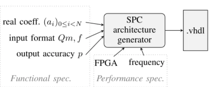
• a very simple interface (Fig. 1) to an implementation tool, focusing designer’s freedom on those design This work is partly supported by the MetaLibm project of the french Agence
Nationale de la Recherche(ANR)
SPC architecture
generator real coeff.(ai)0≤i<N
input formatQm, f output accuracy p
FPGA frequency
.vhdl
Functional spec. Performance spec.
Fig. 1. Interface to the proposed tool.
parameters which are relevant. For instance, it will be shown that the format to which anai will be rounded
is not a relevant design parameter: it can be deduced optimally from the mathematical specification on one side, and the input/output formats on the other side. • a fully automated implementation process that builds
provably-minimal architectures of proven accuracy. A second contribution is an actual open-source tool that demonstrates this implementation process. This tool automat-ically generates VHDL for SPC computations. Built upon the FloPoCo project1, it also benefits from the FloPoCo back-end framework. The generated architectures are optimized for a user-specified FPGA target running at a user-specified frequency (Fig. 1).
A third contribution of this work is to introduce several architectural novelties. The constant multipliers are built using an evolution of the KCM algorithm [1], [2] that manages multiplications by a real constant [3]. The summation is efficiently performed thanks to the BitHeap framework re-cently introduced in FloPoCo [4]. These technical choices lead to logic-only architectures suited even to low-end FPGAs, a choice motivated by work on implementing the ZigBee protocol standard [5] (the examples illustrating this article are from this standard). However, the same philosophy could be used to build other architecture generators, for instance exploiting embedded multipliers and DSP blocks.
II. LAST-BIT ACCURACY:DEFINITIONS AND MOTIVATION
A. Fixed-point formats, rounding errors, and accuracy
Technically, the overall error of a SPC architecture in fixed-point is defined as the difference between the computed value e
y and its mathematical specification:
ǫ = y − ye = y −e
N −1X i=0
aixi (2)
In all the article, we try to use tilded letters (e.g.y above) fore approximate or rounded terms. This is but a convention, and the choice is not always obvious. For instance, here, the xi
are fixed-point inputs, and most certainly the result of some approximate measurement or computation. However, from the point of view of the SPC, they are inputs, they are given, so they are considered exact.
In all the following, we note
• ǫ the error bound, i.e. the maximum of the absolute value ofǫ,
• p the precision of the output format, such that 2−p is
the value of the least-significant bit (LSB) ofy;e • ◦p(x) the rounding of a real x to the nearest
fixed-point number of precision p.
This rounding, in the worst case, entails an error | ◦p(x) − x| < 2−p−1. For instance, rounding a real to the
nearest integer (p = 0) may entail an error up to 0.5 = 2−1.
This is a limitation of the format itself. Therefore, the best we can do, when implementing (1) with a precision-p output, is a
perfectly roundedcomputation with an error boundǫ = 2−p−1.
Unfortunately, since theaiare arbitrarily accurate, reaching
perfect rounding accuracy may require arbitrary intermediate precision. This is not acceptable in an architecture. We there-fore impose a slightly relaxed constraint: ǫ < 2−p. We call
this last-bit accuracy, because the error must be smaller than the value of the last (LSB) bit of the result. It is sometimes called faithful rounding in the literature.
Considering that the output format implies thatǫ ≥ 2−p−1
, it is still a tight specification. For instance, if the exact y happens to be a representable precision-p number, then a last-bit accurate architecture will return exactly this value.
The main reason for chosing last-bit accuracy over perfect rounding is that, as will be shown in Section III, it can be reached with very limited hardware overhead. Therefore, an architecture that is last-bit-accurate top bits makes more sense than a perfectly rounded architecture top−1 bits, for the same accuracy 2−p
.
B. Application-specific architectures should be last-bit accu-rate
The rationale for last-bit accuracy architectures is therefore as follows. On the one hand, last-bit accuracy is the best that the output format allows at acceptable hardware cost. On the other hand, any computation less than last-bit accurate is outputting meaningless bits in the least significant places. If we are designing an architecture, this should clearly be avoided: each output bit has a cost, not only in routing, but also in power and resources downstream, in whatever will process this bit. This price should be paid only for those bits that hold useful information.
C. Real constants for highest-level specification
It is important to emphasize that the ai constants are
considered in this work as infinitely accurate real numbers. In many cases, the coefficients are defined in textbooks by explicit formulas. This is the case for the DCT, but also
for classical signal-processing filters, such as the ones that motivated this work: the half-sine FIR, and the root-raised cosine FIR [5]. In such cases, last-bit accuracy is defined with respect to this purely mathematical specification. Thus the implementation will be as faithful to the maths as the I/O formats allow.
In other cases, we do not have explicit formula, but the coefficients are provided (e.g. in Matlab) as double-precision numbers. In such cases, last-bit accuracy is defined with respect to an infinitely accurate evaluation of (1) using exactly the values provided for the coefficients. In practice, this means that the architecture will behave numerically as if (1) was evaluated by Maple in double precision (or better), with a single rounding of the final result to the output fixed-point format.
When converting a mathematical or Matlab specification to low-precision hardware, last-bit accuracy thus ensures that the hardware is as close to the specification as possible. In addition, it also considerably eases the conversion process itself. Indeed, in a classical design flow, such a conversion involves steps such as coefficient quantization and datapath
dimensioning, which have to be decided by the designer. This requires a lot of effort, typically by trial-and-error until a small enough implementation with a good enough signal-noise ratio is attained. In our approach, as the sequel will show, optimal choices for these steps can be deduced from the specification. Freeing the designer from these time-consuming and error-prone tasks may be the main contribution of this work. It is definitely a progress with respect to most existing DSP tools.
D. Tool interface
To sum up, the ideal interface (Fig. 1) should
• allow a user to input the (ai)0≤i<N to the tool either
as mathematical formulas, or as arbitrary-precision floating-point numbers. Our current implementation only supports the latter so far;
• offer one single integer parameterp, to serve both as accuracy specification and as the definition of the LSB of the output format.
Let us now show that the MSB of the output format, as well as all the internal precision parameters, may be deduced from the parameters depicted on Fig. 1.
III. ENSURING LAST-BIT ACCURACY
The summation of the various terms aixi is depicted on
Fig. 2. For this figure, we take as an example a 4-tap FIR with arbitrary coefficients. As shown on the figure, the exact product of a realaiby an inputximay have an infinite number
of bits.
A. Determining the most significant bit of aixi
A first observation is that the MSB of the products aixi
is completely determined by the ai and the input fixed-point
format. Indeed, we have fixed-point, hence bounded, inputs. If the domain ofxiisxi∈ (−1, 1), the MSB of aixiis the MSB
of|ai|. This is illustrated by Figure 2. In general, if |xi| < M ,
a0= .00001001111111010001010101101... a1= .00101110110001000101001110000... a2= .11000001011011010001001100101... a3= .00110101000001001110111001111... a0x0 xxxxxxxxxxxxxxxxxxxxxxxxx... +a1x1 xxxxxxxxxxxxxxxxxxxxxxxxxxx... +a2x2 xxxxxxxxxxxxxxxxxxxxxxxxxxxxx... +a3x3 xxxxxxxxxxxxxxxxxxxxxxxxxxx... = zzzzzzzzzzzzzzzzzzzzzzzzzzzzzz... y= yyyyyyyyyyyyyyyyyyyyyy 2−p 2−p−g
Fig. 2. The alignment of theaixifollows that of theai
This is obvious if aixi is positive. It is not true if aixi
is negative, since in two’s complement it needs to be sign-extended to the MSB of the result. However the sign extension of a signed number 00...00sxxxx, where s is the sign bit, may be performed as follows:
00...0sxxxxxxx + 11...110000000 = ss...ssxxxxxxx
Here s is the complement of s. The reader may check this equation in the two cases, s= 0 and s = 1. Now the variable part of the product has the same MSB as |ai|.
This transformation is not for free: we need to add a constant. Fortunately, in the context of a summation, we may add in advance all these constants together. Thus the overhead cost of two’s complement in a summation is limited to the addition of one single constant. In many cases, as we will see, this addition can even be merged for free in the computations of the aixi.
B. Determining the most significant bit of the result
A second observation is that the MSB of the result is also completely determined by the(ai)0≤i<N. Again from the
bound |xi| < M , we may deduce that the MSB of the result
is MSBey= & log2( N −1X i=0 |ai|M ) ' . (3)
This upper bound guarantees that no overflow will ever occur.
For this reason, we do not need the user to specify the output MSB on Figure 1: providing the ai is enough.
In some cases, however, the context may dictate a tighter bound due to some additional relationship between thexi, for
instance a consequence of their being successive samples of the same signal. For this reason, the tool offers the option of specifying completely the output format, but this is only an option. Otherwise, the tool will use Eq. (3) to compute the minimal value of the output MSB that guarantees the absence of overflow.
C. Determining the least significant bit: error analysis
As we have seen, a single integerp, the weight of the least significant bit (LSB) of the output, also specifies the accuracy of the computation.
However, performing all the internal computations to this precision would not be accurate enough. Suppose for instance that we could build perfect hardware constant multipliers, returning the perfect rounding pei = ◦p(aixi) of the
math-ematical product aixi to precision p. Even such a perfect
multiplier would entail an error, defined asǫi= epi− aixi, and
bounded by ǫi < ǫmult = 2−p−1. Again this rounding error is
the consequence of the limited-precision output format. The problem is that in a SPC, such rounding errors add up. Let us analyze this.
The output value y is computed in an architecture as thee sum of the pei. This summation, as soon as it is performed
with adders of the proper size, will entail no error. Indeed, fixed-point addition of numbers of the same format may entail overflows (these have been taken care of above), but no rounding error. This enables us to write
e y = N −1X i=0 e pi, (4) therefore ǫ = N −1X i=0 e pi− N −1X i=0 aixi = N −1X i=0 ǫi . (5)
Unfortunately, in the worst case, the sum of the ǫi can
come close toN ǫmult, which, as soon asN > 2, is larger than
2−p: this naive approach is not last-bit accurate.
The solution is, however, very simple. A slightly larger intermediate precision, with g additional bits (“guard” bits) may be used. The error of each multiplier is now bounded by ǫmult= 2−p−1−g. It can be made arbitrarily small by increasing
g. Therefore, there exists some g such that N ǫmult < 2−p−1
Actually, this is true even if a less-than-perfect multiplier architecture is used, as soon as we may compute a boundǫmult
of its accuracy, and this bound is proportional to 2−g.
However, we now have another issue: the intermediate result now hasg more bits at its LSB than we need. It therefore needs itself to be rounded to the target format. This is easy, using the identity◦(x) = ⌊x +1
2⌋: rounding to precision 2 −p
is obtained by first adding 2−p−1 (this is a single bit) then
discarding bits lower than 2−p. However, in the worst case,
this will entail an error ǫfinal rounding of at most2−p−1.
To sum up, the overall error of a faithful architecture SCP is therefore
ǫ = ǫfinal rounding+ N −1X
i=0
ǫi < 2−p−1+ N ǫmult (6)
and this error can be made smaller than 2−p
as soon as we are able to build multipliers such that
N ǫmult < 2−p−1 . (7)
All the previous was quite independent of the target tech-nology: it could apply to ASIC synthesis as well as FPGA. Also, a very similar analysis can be developed for an inner-product architecture where theaiare not constant. Conversely,
the following is more focused on a particular context: LUT-based SCP architectures for FPGAs. It explores architectural
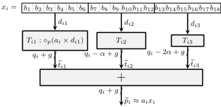
xi= b1 b2 b3 b4 b5 b6 b7 b8 b9b10b11b12b13b14b15b16b17b18 Ti1: ◦p(ai×di1) di1 Ti2 di2 Ti3 di3
+
/ qi+ g e ti1 / qi−α + g eti2 / qi−2α + g e ti3 / qi+ g e pi≈aixiFig. 3. The FixRealKCM method whenxiis split in 3 chunks
means to reach last-bit accuracy at the smallest possible cost, what we call “computing just right” in the title.
IV. AN EXAMPLE OF ARCHITECTURE FORFPGAS On most FPGAs, the basic logic element is the look-up-table (LUT), a small memory addressed by α bits. On the current generation of FPGAs, α = 6.
A. Perfectly rounded constant multipliers
As we have a finite number of possible values for xi, it
is possible to build a perfectly rounded multipliers by simply tabulating all the possible products. The precomputation of table values must be performed with large enough accuracy (using multiple-precision software) to ensure the correct round-ing of each entry. This even makes perfect sense for small input precisions on recent FPGAs: if xi is a 6-bit number,
each output bit of the perfectly rounded product aixi will
consume exactly one 6-input LUTs. For 8-bit inputs, each bit consumes only4 LUTs. In general, for (6 + k)-bit inputs, each output bit consumes 2k
6-LUTs: this approach scales poorly to larger inputs. However, perfect rounding top+g bits means a maximum error smaller than an half-LSB:ǫmult = 2−p−g−1.
Note that for real-valued ai, this is more accurate than using
a perfectly rounded multiplier that inputs ◦p(ai): this would
accumulate two successive rounding errors.
B. Table-based constant multipliers for FPGAs
For larger precisions, we may use a variation of the KCM technique, due to Chapman [1] and further studied by Wirthlin [2]. The original KCM method addresses the multiplication by an integer constant. We here present a variation that performs the multiplication by a real constant.
This method consists in breaking down the binary decom-position of an input xi into n chunks dik of α bits. With the
input size beingm+f , we have n = ⌈(m+f )/α⌉ such chunks (n = 3 on Figure 3). Mathematically, this is written
xi = n X k=1 2−kαd ik where dik∈ {0, ..., 2α− 1} . (8)
The product becomes aixi = n X k=1 2−kαa idik . (9) e ti1= ◦p(aidi1) xxxxxxxxxxxxxxxxxxxxxxxxxx... e ti2= ◦p(aidi2) xxxxxxxxxxxxxxxxxxxx... e ti3= ◦p(aidi3) xxxxxxxxxxxxxx... 2−p 2−p−g α bits α bits
Fig. 4. Aligment of the terms in the KCM method
Since each chunkdik consists of α bits, where α is the LUT
input size, we may tabulate each product aidik in a look-up
table that will consume exactly one α-bit LUT per output bit. This is depicted on Figure 3. Of course, aidik has an infinite
number of bit in the general case: as previously, we will round it to precision 2−p−g. In all the following, we define et
ik =
◦p(aidik) this rounded value (see Figure 4).
Contrary to classical (integer) KCM, all the tables do not consume the same amount of resources. The factor 2−kα
in (9) shifts the MSB of the table output etik, as illustrated by
Figure 4.
Here also, the fixed-point addition is errorless. The error of such a multiplier therefore is the sum of the errors of the n tables, each perfectly rounded:
ǫmult< n × 2−p−g−1 . (10)
This error is proportional to2−g
, so can made as small as needed by increasing g.
C. Computing the sum
In FPGAs, each bit of an adder also consumes one LUT. Therefore, in a KCM architecture, the LUT cost of the summation is expected to be roughly proportional to that of the tables. However, this can be improved by stepping back and considering the summation at the SPC level. Indeed, our faithful SPC result is now obtained by computing a double sum: e y = ◦p N −1X i=0 n X k=1 2−kαet ik ! (11)
Using the associativity of fixed-point addition, this summa-tion can be implemented very efficiently using compression techniques developed for multipliers [6] and more recently applied to sums of products [7], [8]. In FloPoCo, we may use the bit-heap framework introduced in [4]. Each table throws its etik to a bit-heap that is in charge of performing the final
summation. The bit-heap framework is naturally suited to adding terms with various MSBs, as is the case here.
This is illustrated on Fig. 5, which shows the bit heaps for two classical filters from [5]. On these figures, we have binary weights on the horizontal axis, and the various terms to add on the vertical axis. These figure are generated by FloPoCo before bit heap compression.
We can see that the shape of the bit heap reflects the various MSBs of the ai. One bit heap is higher than the other
one, although they add the same number of product and each product should be decomposed into the same number of KCM tables. This is due to special coefficient values that lead to specific optimizations. For instanceai= 1 or ai= 0.5 lead to
Half-Sine Root-Raised Cosine Fig. 5. Bit heaps for two 8-tap, 12-bit FIR filters generated for Virtex-6
Bit-heap based pipelined summation architecture x0 T01 / α T02 / α T03 / α x1 T11 / α T12 / α T13 / α x2 T21 / α T22 / α T23 / α x3 T31 / α T32 / α T33 / α / p y
Fig. 6. KCM-based SPC architecture forN = 4, each input being split into 3 chunks
D. Managing the constant bits
Actually there are two more terms to add to the summation of Eq. (11): the rounding bit 2−p−1, necessary for the final
rounding-by-truncation as explained in Section III-C, and the sum of all the sign-extension constants introduced in Sec-tion III-A. These bits, especially the rounding bit, are visible on Fig. 5.
There is a minor optimization to do here: these constant bits form a binary constant that can be added (at table-filling time) to all the values of one of the tables, for instance T00. Then
the rounding bit will be added for free. The sign extension constants may add a few MSB bits to the table output, hence increase its cost by a few LUTs. Still, with this trick, the summation to perform is indeed given by Eq. (11), and the final rounding, being a simple truncation, is for free. This optimization will be integrated to our implementation before publication.
Finally, the typical architecture generated by our tool is depicted by Figure 6.
E. Pipelining
In terms of speed, reading the table values takes one LUT delay, this is as fast as it gets on an FPGA. The summation, however, may have a significant delay – at most that of N − 1 additions, but much less in practice thanks to efficient compressor architectures on recent FPGAs. In any cases, the BitHeap framework takes care of the pipelining.
For instance, when using the previous to implement a FIR, we obtain the architecture of Fig. 7. Pipelining the summation may add some latency to the operator, especially compared to an inverted design. However, the bit-heap saves area by
xi xi−1 xi−2 xi−3
yi−2
Fig. 7. A pipelined FIR – thick lines denote pipeline levels
Taps I/O size Speed Area 8 12 bits 4.4 ns (227 Mhz) 564 LUT
1 cycle @ 344 Mhz 594 LUT 32 Reg. 8 18 bits 5.43ns (184 MHz) 1325 LUT
2 cycles @ 318 MHz 1342 LUT 92Reg. 16 12 bits 5.8 ns (172 Mhz) 1261 LUT
1 cycle @ 289 Mhz 1257 LUT 41 Reg. 16 18 bits 7.3 ns (137 MHz) 2863 LUT
2 cycles @ 265 MHz 2810 LUT 120 Reg. Note: the register count does not include the input shift register.
TABLE I. SYNTHESIS RESULTS OF AROOT-RAISEDCOSINEFIR.
optimizing the summation globally, instead of considering as a sequence of additions.
V. IMPLEMENTATION AND RESULTS
The method described in this paper is implemented as the FixFIR operator of FloPoCo. FixFIR offers the interface shown on Fig. 1, and inputs the ai as arbitrary-precision
numbers. On top of it, the operators FixHS and FixRRCF simply evaluate the ai using the textbook formula for
Half-Sine and Root-Raised Cosine respectively, and feed them to FixFIR. We expect many more such wrappers could be written in the future.
FixFIR, like most FloPoCo operators, was designed with a testbench generator [9]. All these operators reported here have been checked for last-bit accuracy by extensive simula-tion.
Table I reports synthesis results for architectures generated by FixRRCF, as of FloPoCo SVN revision 2666. All the results were obtained for Virtex-6 (6vhx380tff1923-3) using ISE 14.7. These results are expected to improve in the future, as the (still new) bit-heap framework is tuned in FloPoCo.
A. Analysis of the results
As expected, the dependency of the area to the number of taps is almost linear. On the one hand, more taps increase the number of needed guard bits. On the other hand, more taps mean a larger bit heap which exposes more opportunities for efficient compression. However, there is also the dependency of the ai themselves to the number of taps.
Conversely, the dependency of area on precision is more than linear. It is actually expected to be almost quadratic, as can be observed by evaluating the number of bits tabulated for each multiplier (see Fig. 4).
Interestingly, the dependency of the delay to the number of taps is clearly sub-linear. This is obvious from Fig. 6. All the table accesses are performed in parallel, and the delay is dominated by the compression delay, which is logarithmic in the bit-heap height [10].
B. Comparison to a naive approach
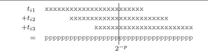
In order to evaluate the cost of computing just right, we built a variant of the FixFIR operator following a more classical approach. In this variant, we first quantize all the coefficients to precision p (i.e such that their LSB has weight 2−p
). We obtain fixed-point constants, and we then build an architecture that multiplies these constants with the inputs using the classical (integer) KCM algorithm.
A simple error analysis shows that the mere quantization to precision p is already responsible for the loss of two bits of accuracy on y. The exact error due to coefficiente quantization depends on the coefficients themselves but space is missing here to detail that. Then, the multiplications are exact. However, as illustrated by Figure 8, their exact results extend well below precision 2p
: they have to be rounded. We just truncate the output of each KCM operators to 2−p. This
more than doubles the overall error. It also allows the synthesis tools to optimize out the rightmost 6 bits of Fig. 8. Then these truncated products are summed using a sequence of N − 1 adders of precisionp.
The results are visible in Table II. The naive approach leads to a much smaller, but slower design. The area difference doesn’t come from the tables, if we compare Fig. 4 and Fig. 8. It comes from the summation, which is performed ong more bits in the bit accurate approach. Besides, only the last-bit accurate approach uses a last-bit heap, whose compression heuristics are currently optimized for speed more than for area. However, this comparison is essentially meaningless, since the two architectures are not functionally equivalent: The proposed approach is accurate to 12 bits, while the naive approach loses more than 3 bits to quantization and truncation. Therefore, a meaningful comparison is the proposed approach, but accurate to p = 9, which we also show in Table II. This version is better than the naive one in both area and speed.
Since we are comparing two designs by ourselves, it is always possible to dispute that we deliberately sabotaged our naive version. This is right, in a sense. We designed it as small as possible (no guard bits, truncation instead of rounding, etc). Short of designing a filter that returns always zero (very poor accuracy, but very cheap indeed), this is the best we can do. But all these choices are highly disputable, in particular because they impact accuracy.
All this merely illustrates the point we want to make: it only makes sense to compare designs of equivalent accuracies. And the only accuracy that makes sense is last-bit accuracy, for the reasons exposed in II-B. We indeed put our best effort in designing the last-bit accurate solution, and we indeed looked for the most economical way of achieving a given accuracy. This is comforted by this comparison. Focussing on last bit accuracy enables us to compute right, and just right.
For the sake of completeness, we also implemented a version using DSP blocks, reported in Table II. Considering
ti1 xxxxxxxxxxxxxxxxxxxxxxxx
+ti2 xxxxxxxxxxxxxxxxxxxxxxxx
+ti3 xxxxxxxxxxxxxxxxxxxxxxxx
= pppppppppppppppppppppppppppppppppppp 2−p
Fig. 8. Using integer KCM:tik = ◦p(ai) × dik. This multiplier is both
wasteful, and not accurate enough.
Method Speed Area accuracy p = 12, proposed 4.4 ns (227 Mhz) 564 LUT ǫ < 2−12
p = 12, naive 5.9 ns (170 Mhz) 444 LUT ǫ > 2−9
p = 9, proposed 4.12 ns (243 Mhz) 380 LUT ǫ < 2−9
p = 12, DSP-based 9.1 ns (110 Mhz) 153 LUT, 7 DSP ǫ < 2−9 TABLE II. THE ACCURACY/PERFORMANCE TRADE-OFF ON8-TAP, 12
BITROOT-RAISEDCOSINEFIRFILTERS.
the large internal precision of DSP blocks, it costs close to nothing to design this version as last-bit accurate for p = 12 or p = 18 (in the latter case, provided the constant is input with enough guard bits on the 24-bit input of the DSP block). This is very preliminary work, however. We should offer the choice between either an adder tree with a shorter delay, or a long DSP chain which would be slow, but consume no LUT. We should also compare to Xilinx CoreGen FIR compiler, which generates only DSP-based architectures. Interestingly, this tool requires the user to quantize the coefficients and to take all sorts of decisions about the intermediate accuracies and rounding modes.
CONCLUSION
This paper claims that sum-of-product architectures should be last bit accurate, and demonstrates that this has two positive consequences: It gives a much clearer view on the trade-off between accuracy and performance, freeing the designer from several difficult choices. It actually leads to better solutions by enabling a “computing just right” philosophy. All this is demonstrated on an actual open-source tool that offers the highest-level interface.
Future work include several technical improvements to the current implementation, such as the exploitation of symmetries in the coefficients or optimization of the bit heap compression.
Beyond that, this work opens many perspectives.
As we have seen, fixed-point sum of products and sum of squares could be optimized for last-bit accuracy using the same approach.
We have only studied one small corner of the vast liter-ature about filter architecture design. Many other successful approaches exist, in particular those based on multiple constant multiplication (MCM) using the transpose form (where the registers are on the output path). [11], [12], [13], [14], [15]. A technique called Distributed Arithmetic, which predates FPGA [16], can be considered a generalization of the KCM technique to the MCM problem. From the abstract of [17] that, among other things, compares these two approaches, “if the input word size is greater than approximately half the number of coefficients, the LUT based multiplication scheme needs less resources than the DA architecture and vice versa”. Such a
rule of thumb (which of course depends on the coefficients themselves) should be reassessed with architectures computing just right on each side. Most of this vast literature treats accuracy after the fact, as an issue orthogonal to architecture design.
A repository of FIR benchmarks exists, precisely for the purpose of comparing FIR implementations [18]. Unfortu-nately, the coefficients there are already quantized, which prevents a meaningful comparison with our approach. Few of the publications they mention report accuracy results. However, cooperation with this group should be sought to improve on this.
We have only considered here the implementation of a filter once the ai are given. Approximation algorithms, such
as Parks-McClellan, that compute these coefficients, essentially work in the real domain. The question they answer is “what is the best filter with real coefficients that matches this specifica-tion”. It is legitimate to wonder if asking the question: “what is the best filter with low-precision coefficients” could not lead to a better result.
Still in filter design, the approach presented here should be extended to infinite impulse response (IIR) filters. There, a simple worst-case analysis (as we did for SPC) doesn’t work due to the infinite accumulation of error terms. However, as soon as the filter is stable (i.e. its output doesn’t diverge), it should be possible to derive a bound on the accumulation of rounding errors. This would be enough to design last-bit accurate IIR filters computing just right.
REFERENCES
[1] K. Chapman, “Fast integer multipliers fit in FPGAs (EDN 1993 design idea winner),” EDN magazine, no. 10, p. 80, May 1993.
[2] M. Wirthlin, “Constant coefficient multiplication using look-up tables,”
Journal of VLSI Signal Processing, vol. 36, no. 1, pp. 7–15, 2004. [3] F. de Dinechin, H. Takeugming, and J.-M. Tanguy, “A 128-tap complex
FIR filter processing 20 giga-samples/s in a single FPGA,” in 44th
Asilomar Conference on Signals, Systems & Computers, 2010. [4] N. Brunie, F. de Dinechin, M. Istoan, G. Sergent, K. Illyes, and B. Popa,
“Arithmetic core generation using bit heaps,” in Field-Programmable
Logic and Applications, Sep. 2013.
[5] IEEE Std 802.15.4-2006, IEEE Standard for Information technology–
Telecommunications and information exchange between systems– Local and metropolitan area networks– Specific requirements– Part 15.4: Wireless Medium Access Control (MAC) and Physical Layer (PHY) Specifications for Low-Rate Wireless Personal Area Networks (WPANs), 2006.
[6] M. D. Ercegovac and T. Lang, Digital Arithmetic. Morgan Kaufmann, 2003.
[7] H. Parendeh-Afshar, A. Neogy, P. Brisk, and P. Ienne, “Compressor tree synthesis on commercial high-performance FPGAs,” ACM Transactions
on Reconfigurable Technology and Systems, vol. 4, no. 4, 2011. [8] R. Kumar, A. Mandal, and S. P. Khatri, “An efficient arithmetic
sum-of-product (SOP) based multiplication approach for FIR filters and DFT,” in International Conference on Computer Design (ICCD). IEEE, Sep. 2012, pp. 195–200.
[9] F. de Dinechin and B. Pasca, “Designing custom arithmetic data paths with FloPoCo,” IEEE Design & Test of Computers, vol. 28, no. 4, pp. 18–27, Jul. 2011. [Online]. Available: http: //ieeexplore.ieee.org/xpls/abs all.jsp?arnumber=5753874
[10] L. Dadda, “Some schemes for parallel multipliers,” Alta Frequenza, vol. 34, pp. 349–356, 1965.
[11] M. Potkonjak, M. Srivastava, and A. Chandrakasan, “Efficient sub-stitution of multiple constant multiplications by shifts and additions using iterative pairwise matching,” in ACM IEEE Design Automation
Conference, San Diego, CA USA, 1994, pp. 189–194.
[12] N. Boullis and A. Tisserand, “Some optimizations of hardware multipli-cation by constant matrices,” IEEE Transactions on Computers, vol. 54, no. 10, pp. 1271–1282, 2005.
[13] M. Mehendale, S. D.Sherlekar, and G. Venkatesh, “Synthesis of multiplier-less FIR filters with minimum number of additions,” in
IEEE/ACM International Conference on Computer-Aided Design, San Jose, CA USA, 1995, pp. 668–671.
[14] Y. Voronenko and M. P¨uschel, “Multiplierless multiple constant multi-plication,” ACM Trans. Algorithms, vol. 3, no. 2, 2007.
[15] L. Aksoy, E. Costa, P. Flores, and J. Monteiro, “Exact and approximate algorithms for the optimization of area and delay in multiple constant multiplications,” IEEE Transactions on Computer-Aided Design of
Integrated Circuits and Systems, vol. 27, no. 6, pp. 1013–1026, 2008. [16] S. White, “Applications of distributed arithmetic to digital signal processing: A tutorial review,” IEEE ASSP Magazine, no. 3, pp. 4–19, Jul. 1989.
[17] M. Kumm, K. M¨oller, and P. Zipf, “Dynamically reconfigurable FIR filter architectures with fast reconfiguration,” in Reconfigurable and
Communication-Centric Systems-on-Chip (ReCoSoC). IEEE, Jul. 2013. [18] “FIR suite,” http://www.firsuite.net/.