Publisher’s version / Version de l'éditeur:
Vous avez des questions? Nous pouvons vous aider. Pour communiquer directement avec un auteur, consultez la première page de la revue dans laquelle son article a été publié afin de trouver ses coordonnées. Si vous n’arrivez Questions? Contact the NRC Publications Archive team at
PublicationsArchive-ArchivesPublications@nrc-cnrc.gc.ca. If you wish to email the authors directly, please see the first page of the publication for their contact information.
https://publications-cnrc.canada.ca/fra/droits
L’accès à ce site Web et l’utilisation de son contenu sont assujettis aux conditions présentées dans le site
LISEZ CES CONDITIONS ATTENTIVEMENT AVANT D’UTILISER CE SITE WEB. Technical Report; no. TR-2004-06, 2004
READ THESE TERMS AND CONDITIONS CAREFULLY BEFORE USING THIS WEBSITE. https://nrc-publications.canada.ca/eng/copyright
NRC Publications Archive Record / Notice des Archives des publications du CNRC :
https://nrc-publications.canada.ca/eng/view/object/?id=290e8976-22ee-4216-9721-128694219c76 https://publications-cnrc.canada.ca/fra/voir/objet/?id=290e8976-22ee-4216-9721-128694219c76
Archives des publications du CNRC
For the publisher’s version, please access the DOI link below./ Pour consulter la version de l’éditeur, utilisez le lien DOI ci-dessous.
https://doi.org/10.4224/8895251
Access and use of this website and the material on it are subject to the Terms and Conditions set forth at Preliminary CFD Study of Model Induced Circulation in the IMD Clearwater Towing Tank
REPORT NUMBER
TR-2004-06
NRC REPORT NUMBER DATE
June 2004
REPORT SECURITY CLASSIFICATION
Unclassified
DISTRIBUTION
Unlimited
TITLE
PRELIMINARY CFD STUDY OF MODEL INDUCED
CIRCULATION IN THE IMD CLEARWATER TOWING TANK
AUTHOR(S)
Eric Thornhill, Rob Pallard, Caroline Muselet
CORPORATE AUTHOR(S)/PERFORMING AGENCY(S)
Institute for Ocean Technology, Memorial University of Newfoundland
PUBLICATION
SPONSORING AGENCY(S)
Institute for Ocean Technology, Memorial University of Newfoundland
IOT PROJECT NUMBER NRC FILE NUMBER
KEY WORDS
Circulation, Towing Tank, Baffles
PAGES v, 33, App. A FIGS. 44 TABLES 2 SUMMARY
It was observed when testing large models of sailing yachts in the NRC/IMD towing tank that lasting flow patterns were being produced in the tank, which could affect force measurements. Some assessments of the phenomena were made, but the nature of the flow was not well understood. Attempts to minimize the circulation effects on model testing were primarily made by trial and error. This report presents results from a preliminary CFD study (2D) of the dynamics of this induced flow.
ADDRESS National Research Council Institute for Ocean Technology Arctic Avenue, P. O. Box 12093 St. John's, NL A1B 3T5
Institute for Ocean Institut des technologies
Technology océaniques
PRELIMINARY CFD STUDY OF MODEL INDUCED
CIRCULATION IN THE IMD CLEARWATER TOWING TANK
TR-2004-06
Eric Thornhill Rob Pallard Caroline Muselet
TABLE OF CONTENTS
List of Tables ... iv
List of Figures ... iv
1.0 INTRODUCTION...1
2.0 BACKGROUND ...1
3.0 TANK & MODEL DETAILS...3
4.0 CIRCULATION MEASUREMENTS...5 5.0 CFD SIMULATIONS ...7 5.1 No Baffles ...9 5.2 Baffles A ...13 5.3 Baffles B ...19 5.4 Baffles C ...23 5.5 Side Baffle ...26 5.6 Other Simulations ...29 6.0 DISCUSSION...29 7.0 CONCLUSIONS...33
LIST OF TABLES
Page
Table 1: Typical Model Particulars ... 4
Table 2: Normalized Average Velocity at End of Simulation ... 33
LIST OF FIGURES Page Figure 1: Typical Sailing Yacht ...4
Figure 2: Plan View of Towing Tank (7m deep) ...5
Figure 3: Tank & Measurement Points...6
Figure 4: Tank Current Measurements3 (Model Speed = 2.74m/s, Yaw Angle 3°)7 Figure 5: Keel and Velocity Components...7
Figure 6: Tank Dimensions ...8
Figure 7: Grid Detail at Tank Corner ...9
Figure 8: No Baffles: Velocity Magnitude Contours (Time = 0.4 sec.)...10
Figure 9: No Baffles: Velocity Magnitude Contours (Time = 12 sec.)...10
Figure 10: No Baffles: Velocity Magnitude Contours (Time = 64 sec.)...11
Figure 11: No Baffles: Velocity Magnitude Contours (Time = 152 sec.)...11
Figure 12: No Baffles: Velocity Magnitude Contours (Time = 340 sec.)...12
Figure 13: No Baffles: Velocity Magnitude Contours (Time = 932 sec.)...12
Figure 14: No Baffles: Vortex Center Path...13
Figure 15: Grid Detail at Baffle/Wall Junction ...14
Figure 16: Baffles A: Velocity Magnitude Contours (Time = 0.4 sec.) ...15
Figure 17: Baffles A: Velocity Magnitude Contours (Time = 32 sec.)...15
Figure 18: Baffles A: Velocity Magnitude Contours (Time = 280 sec.) ...16
Figure 19: Baffles A: Velocity Magnitude Contours (Time = 932 sec.) ...16
Figure 20: Baffles A: Vortex Centers’ Paths...17
LIST OF FIGURES (cont'd)
Page
Figure 22: Flow Velocity in X-Direction 1.4m below Water Surface ...18
Figure 23: Flow Direction Y-Direction 1.4m below Water Surface ...19
Figure 24: Baffles B: Velocity Magnitude Contours (Time = 0.4 sec.) ...20
Figure 25: Baffles B: Velocity Magnitude Contours (Time = 14 sec.)...20
Figure 26: Baffles B: Velocity Magnitude Contours (Time = 208 sec.) ...21
Figure 27: Baffles B: Velocity Vectors (Time = 208 sec.) ...21
Figure 28: Baffles B: Velocity Magnitude Contours (Time = 932 sec.) ...22
Figure 29: Baffles B: Vortex Centers’ Paths...22
Figure 30: Baffles C: Velocity Magnitude Contours (Time = 0.4 sec.)...23
Figure 31: Baffles C: Velocity Magnitude Contours (Time = 100 sec.)...24
Figure 32: Baffles C: Velocity Magnitude Contours (Time = 272 sec.)...24
Figure 33: Baffles C: Velocity Magnitude Contours (Time = 932 sec.)...25
Figure 34: Baffles C: Vortex Centers’ Paths ...25
Figure 35: Side Baffle: Velocity Magnitude Contours (Time = 0.4 sec.) ...26
Figure 36: Side Baffle: Velocity Magnitude Contours (Time = 92 sec.)...27
Figure 37: Side Baffle: Velocity Magnitude Contours (Time = 412 sec.) ...27
Figure 38: Side Baffle: Velocity Magnitude Contours (Time = 932 sec.) ...28
Figure 39: Side Baffle: Vortex Centers’ Paths...28
Figure 40: Test Section Dimensions ...30
Figure 41: No Baffles: Average Velocities...31
Figure 42: Average Velocities in Entire Tank Cross-Section...32
Figure 43: Average Velocities in Test Section ...32
Preliminary CFD Study of Model Induced
Circulation in the IMD Clearwater Towing Tank
Eric Thornhill, Rob Pallard, Caroline Muselet
1.0 INTRODUCTION
The National Research Council of Canada’s Institute for Marine Dynamics (NRC/IMD) is an experimental facility, which, among other activities, performs model scale testing of sailing yachts. The goal of this testing is usually to assess the resistance characteristics of a hull shape, and the performance of a keel arrangement. The differences between models can often be subtle, so precise force measurements are required to ensure accurate
evaluations.
Despite a sophisticated force dynamometer, it was observed that test results for identical runs could vary with the time of day, or with other factors associated with the number and type of preceding tests. After an investigation it was observed that currents at various depths were forming by the successive passage of the model that dissipated at much slower rates than the surface waves. This circulation was then influencing the hydrodynamics of the model and hence the force measurements.
Several trial and error approaches were attempted to minimize these effects including several baffle arrangements. The most successful arrangement consisted of a pair of longitudinal semi-porous baffles at the bottom center of the tank.
It was not possible at the time to make a detailed quantitative map of the flow patterns with time histories, though a few point measurements were made. As a result, the
dynamics of the circulation were not well understood. This paper presents the results of a preliminary CFD study where the flow dynamics were examined for a 2D transverse section of the tank using the commercial software FLUENT (v6.0).
2.0 BACKGROUND
In 1993, IMD was contracted to perform an extensive set of model experiments for the oneAustralia syndicate for the 1995 America’s Cup. In preparation for this project, a series of ‘wait time’ (the time between individual model tests) experiments were performed as part of an effort to establish a test methodology enabling repeatability of better that 0.5% on drag. These experiments were done at zero leeway with a 1:2.8 scale model of the canoe body (hull without rudder or keel) of an America’s Cup yacht. This work is the basis of the wait time scheme still in use at IMD. These experiments, however, did not address the effects of side force1 on wait time. As the oneAustralia program progressed, poor repeatability of runs done after tests at high speed and side force was observed. Circulation was identified as being the cause very early on in the experiments, but the client’s representative refused to consider that this might be the problem. This opinion was reinforced by conversations with personnel at a number of
1
other test facilities who had never heard of such a thing affecting test results and suggested that the people at IMD should look harder at their test equipment before considering this option.
During the course of the program, it was found that increasing wait time reduced the data variability, but that the resulting test schedule was no longer economically or technically feasible. At the end of that program, the client agreed to accept the data measured at zero leeway. However, before oneAustralia would consider returning to IMD, a solution would have to be found for the problem data variability.
Circulation was identified initially, qualitatively, by use of tell-tales. Approximately 8 evenly spaced tell-tales were mounted on a vertical pole located at mid-tank length, about 2lm from the sidewall. It was observed after a high side force run that tell-tales at the top and bottom of the pole indicated current in opposite directions. Later, the magnitude of the circulation was measured with a 3-axis ultrasonic probe placed in the centerline of the tank about 0.5lm above the bottom of the tank. Some time after the model went by, the transverse flow there was measured to be about 8lcm/s. While data variability correlated well with the magnitude of the transverse flow at the bottom of the tank, there was no simple way to incorporate it into the analysis procedure. Also, there was a lack of
willingness to alter the whole test program on the performance of a single current probe.
It was also noted that a transverse flow of about 3 mm/s, in the area of the foils, would have been sufficient to cause the unwanted behaviour, and that the problem was less noticeable if side force was less than about 700 N. Typical upwind side forces at the 1:2.8 scale were about 1100-1200 N and the oneAustralia test matrix had many runs where side force was in excess of the 2000 N. To put this amount of side force in perspective, the drag at 16 knots full scale was about 1200 N. The client’s experience base was mainly at a scale of 1:3.5 and hence forces were approximately half what were being measured at IMD.
During the same period, knowing the opinion expressed by personnel at other tanks, differences between the IMD tank and other test facilities were compared. It was noticed that the width/depth ratio of the IMD tank cross-section was lower than most other tow tanks and significantly lower than the tank with which the client representative had much experience. An experiment was then done in the IMD Ice Tank, which has a higher width/depth ratio (the same width as the tow tank, but only half the depth). Data
variability was reduced to an acceptable level, but a full experimental series could not be performed in the Ice Tank because of limited speed and run length. A practical solution was therefore needed for use in the towing tank.
This experiment did give an insight into one way of handling the problem. Options considered for altering the tank width/depth ratio include reducing the water level or installing a false floor. These were discarded primarily because of cost and practicality. Lowering water depth would have required a substantial extension to the yacht
achieve. A false floor over the 130lm of available run length would have been far too costly, as well as impeding much of the other work scheduled for the facility.
During the fall of 1993, experiments were conducted at the MUN OERC2 tow tank (58m long, 4.5m wide, 2.2m deep) on a foil & bulb combination attached to a small apparatus that measured lift and drag. A series of experiments were performed at various wait times and water depths. The goal was to determine whether this phenomenon was limited to large tanks or if it could be produced in a small tank. The tests showed that this was indeed possible, confirming previous beliefs that circulation was responsible for the variability problem. Ideas for circulation reduction in the IMD tow tank were then proposed, including the use of plastic snow fencing positioned longitudinally down the tank bottom as a mean of breaking up and dissipating transverse velocities.
Support for the snow fencing was provided by standard scaffolding units, used for their relatively low cost and the ease with which they could be installed or repositioned in the tank. The scaffolding units (approx. 3 m high and 1.5 m wide) were sided with the snow fencing and placed at the center of the tank floor running nearly the full length of the tank. A scale version of the scaffolding approach was built and tested in the MUN tank and the results were promising enough that IMD rented, and eventually bought, enough scaffolding to implement the system. Tests performed in December of 1993 showed that IMD could achieve a level of repeatability that was acceptable to the client.
Since then, it was observed that viscosity has a significant effect on circulation and the limit when baffles become necessary to improve repeatability. Viscosity may have been the most important factor in why the tests in the Ice Tank showed so much promise (water temperature was likely around 4° C compared with about 17° C in the towing tank). Unfortunately, it wasn’t measured during these tests; the goal then was only to assess data variability and not to expand the data to full scale. Tests done at the Naval Surface Warfare Center in Carderock, MD with variations on the IMD baffle system showed similar results as obtained at IMD. However, wait times tended to be slightly longer, partly due to the wider cross-section and greater length of the tank, but also to the higher temperature, and hence lower viscosity, of the water in that facility.
3.0 TANK & MODEL DETAILS
The NRC/IMD towing tank, shown in Figure 2, is 200 m long, 12 m wide, 7 m deep and contains fresh water. Models are attached to a tow carriage, which has a maximum speed of 10.0 m/s with accelerations available in steps of 0.2 m/s2 up to 1.2 m/s2.
A typical yacht model shown in Figure 1, with particulars given in Table 3. It is attached to the carriage by means of a specially designed yacht dynamometer that holds the model at a specified yaw, and roll angle (to simulate a sailing yacht’s typical at-speed orientation), while measuring quantities such as lift, drag, roll moment, yaw moment. The dynamometer permits the model to be free to pitch and heave while constraining it in
2
surge, sway, roll, and yaw. The preferred test displacement is about 900-1200 kg. Lighter models can be accommodated by use of a counterweight apparatus.
Design Scale Speed (kts FS) Length (m) Displacement (kg) Draft (m) IACC 2.8 - 3 2 - 18 6 - 6.5 900 - 1200 1.33 - 1.43 W60 - V60 2.4 - 2.8 4 - 23 6.5 - 7.6 900 - 1400 1.43 - 1.67 IMS 1.85 - 2.3 2 - 20 5.4 - 7.8 800 - 1400 1.4 - 1.6 Table 3: Typical Model Particulars
Appendage configurations tested include typical IACC monoplane with bulb and winglets; W60 L-type and T-type keel bulb arrangements; tandems, forward rudders, simple IMS style keels and keel/centerboard configurations.
A typical test program consists of a series of runs covering the expected speed range for the design at several heel angles and zero leeway. In addition, runs are made to cover the expected range of upwind and reaching sailing conditions. Test schedule (wait time) is a function of the speed and leeway of the previous run. Since it is necessary that the model adopt the same attitude as the full scale yacht, ballast is shifted longitudinally to
compensate for the difference in height between the model tow point and the vertical center of effort of the sail plan. For tests with the model heeled and at leeway, the estimate of side force is used to calculate the vertical force that must be added to the model to compensate for the upward force of the lift generated by the appendages.
Hydraulics Pit Wave Maker
Underwater
Video Camera Carriage Wave Absorber(Beach) Trim Docks
200m 118m 20m 14m 5m 12m
Figure 2: Plan View of Towing Tank (7m deep)
4.0 CIRCULATION MEASUREMENTS
In September 2002, during tests conducted with the IMD standard yacht model at various yaw angles, flow velocity was measured at two points at a position 124m down the length of the tank (near the middle of the model run length). The tank and
measurement points (3m from the tank wall, 0.7m & 1.4m below the water surface) are shown in Figure 3.
At the 1.4m measurement point, a 3D Sontek Acoustic Doppler Velocimeter was used. Measurement with this probe requires the presence of particles, or seeding material, in the water. This was achieved by locally adding chlorine powder around the probe prior to each measurement.
At the 0.7m measurement point, a prototype of an IMD-designed instrument was employed. A wiffle ball, a slightly buoyant hollow plastic sphere covered with small holes, was mounted at the top end of a hinged arm supporting an accelerometer. Current in the water generated drag on the ball, which tipped the arm over. The value of tip angle, as reported indirectly by the accelerometer, correlates to the velocity magnitude of the flow. The instrument was oriented to respond to current transversely across the tank (due to its design, this probe may have also responded to a vertical component of current). Calibration was performed at the end of the test program by mounting the instrument on the carriage and towing it at various speeds in the water.
5.25m 1.5m 5.25m 7m 3m 1.4m 0.7m 3m Water Surface Baffles Sontek Probe Wiffle Ball Probe Y X
Figure 3: Tank & Measurement Points
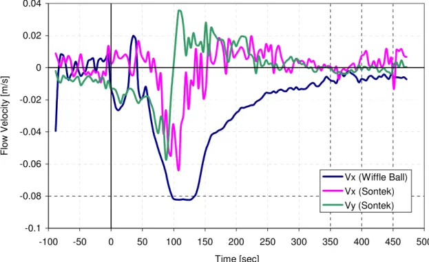
Figure 43 shows the time responses of the probes during a run with a yawed yacht model (time = 0 sec. corresponds to the time when the model passes the probes). Just after the model passes, the upper point registers a pulse of flow towards the left tank wall. More than a minute later both points experienced a longer and more pronounced flow, again towards the left tank wall. The Sontek probe also showed that the vertical component of flow changed direction partway through the pulse. The flow was measurable for several minutes before settling back into the ambient level for the instruments (the Sontek probe showed high levels of noise depending on the quantity of seeding material present).
Circulation currents were observed visually at the same time as a result of the chlorine particles used to seed the water for the acoustic probe. During the period of pronounced flow measured by the instruments, a strong wake was seen around the support rod for the probes. As the wiffle ball tipped, the chlorine particles were observed to travel quickly towards the left wall, and then curve down the wall and back towards the centerline of the tank at a greater depth. The diameter of this large observed circulation pattern was
estimated between 4-5m.
3
There was some uncertainty as to the direction of flow measured by the Vx Sontek probe. It is presented here as being predominately in the negative x-direction, though it could possibly be reversed in sign.
-0.1 -0.08 -0.06 -0.04 -0.02 0 0.02 0.04 -100 -50 0 50 100 150 200 250 300 350 400 450 500 Time [sec] Flow Velocity [m/s] Vx (Wiffle Ball) Vx (Sontek) Vy (Sontek)
Figure 4: Tank Current Measurements (Model Speed = 2.74m/s, Yaw Angle 3°)
5.0 CFD SIMULATIONS
The CFD simulations were performed using the commercial software FLUENT (v6.0), an unstructured RANS code using finite volume discretization. It was decided to first attempt 2D simulations of a transverse section of the tank to see if initial assumptions of the flow were reasonable.
Since the model would be passing perpendicular to the plane of the simulation, an artificial device was needed to initiate the flow. This was done by considering only the effects of the keel, which due to the orientation of the model, runs at an angle of attack down the tank producing side forces, and velocities in the transverse plane. This is shown in Figure 5; only the y-velocity component was considered in the simulations.
A transverse section of the tank was created as a 2D plane. To model the disturbance caused by the passing keel, a small area (called the ‘set zone’) was formed at the location where the keel would pass through the transverse plane. The cells in this region could then be set to a fixed velocity or left alone. During the first two seconds of the simulation (initialization period) the set zone cells were assigned a horizontal velocity equal to 1.0 m/s (from right to left). The vertical velocity was set to zero. This velocity magnitude was estimated based on knowledge of the flow currents, all other water in the tank was considered initially quiescent. After these first two seconds, the fixed cells would take on velocities assigned by the solver according to the equations of conservation of mass and momentum. The flow was then allowed to develop without external influence for approximately 15 minutes of simulation time (roughly the wait time between successive model test runs). The tank and set zone are shown below in Figure 6.
Figure 6: Tank Dimensions
The 2D unstructured grid was created in GAMBIT. A boundary layer grid was created on all of the tank walls (first row was set at 1mm, 10 rows with a growth factor of 1.3). The details of the boundary layer mesh at a tank corner are shown in Figure 7. The rest of the interior of the tank was meshed with an unstructured triangular grid with an average face size of 0.1m. Typical meshes contained approximately 23,000 cells. The left, right, and bottom walls of the tank were assigned the ‘no-slip’ boundary condition. The top wall, which should be a free surface, was given a zero shear-stress (or ‘free slip’) boundary condition.
Simulations were conducted using FLUENT’s 1st order unsteady (transient) solver with the ‘laminar’ viscous option (no turbulence modeling). Addition solver settings for a typical simulation are given in Appendix A.
A simulation would begin with a quiescent tank except for the set zone, which would be assigned a horizontal velocity of –1.0m/s. Two seconds of simulation time would then run with a timestep size of 0.1 seconds. After this period, the forced velocity in the set
zone would be turned off. The flow would then continue for: 60 timesteps at 0.5 sec., and 900 timesteps at 1.0 sec (for a total of 15.5 minutes of simulation time). Data files were saved every four timesteps.
Figure 7: Grid Detail at Tank Corner
5.1 No Baffles
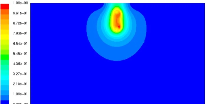
The no baffles case is as shown in Figure 6. During the initiation phase (the first two seconds of the simulation) two vortices are formed on the top and bottom area of the set zone, as shown in Figure 9. The top vortex is rotating clockwise, and the bottom vortex counterclockwise (flow in the set zone is from right to left). These were considered to roughly model the vortices shed from the bottom of the keel and from the hull body. Shortly after the set zone is turned off, the top vortex diminishes as it moves right with most of its momentum attaching to the top (free slip) boundary. The bottom vortex (primary vortex) grows larger and more coherent as it moves to the left. As the left side of the vortex is approaches the left wall, it changes direction and begin moving
downward (Figure 11). Still growing, the outer edge is soon in contact with the bottom wall and the vortex then moves right toward the center of the tank. As it moves right, it’s path then takes it slightly upwards until the vortex center reaches the center of the tank where it remains for the duration of the simulation. The vortex itself was not uniform, as can be seen in the figures, there was a distinct region of localized higher velocity; a remnant of the set zone that created it. As the vortex began moving toward to center itself in the tank, this region tended to smear and become less distinct.
Figure 8: No Baffles: Velocity Magnitude Contours (Time = 0.4 sec.)
Figure 10: No Baffles: Velocity Magnitude Contours (Time = 64 sec.)
Figure 12: No Baffles: Velocity Magnitude Contours (Time = 340 sec.)
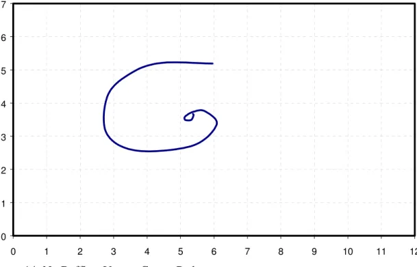
0 1 2 3 4 5 6 7 0 1 2 3 4 5 6 7 8 9 10 11 12
Figure 14: No Baffles: Vortex Center Path
5.2 Baffles A
The next simulation of the tank included a set of longitudinal running baffles of the same dimensions of those currently used for yacht studies. They were centered at the bottom of the tank 1.5lm apart and were 3.0lm high. The actual baffles are a type of plastic fencing (normally used to prevent snow drifting on highways) held on standard scaffolding units. As a simplification, the baffles in the simulation were treated as 1 dimensional solid walls. The meshing strategy was the same as for the no baffles case, except that no boundary layer grid was applied to the baffles. Figure 15 shows the mesh at the baffle/bottom wall junction.
Baffle
Figure 15: Grid Detail at Baffle/Wall Junction
The simulation was initiated in the same manner as the no baffles case by fixing velocities in the set zone. The same starting flow pattern was produced, but the influence of the baffles was seen very early on as shown in the difference between Figure 16 and Figure 8. After the initiation period, the bottom vortex then began moving left as before, but tended more linearly then the no-baffles case and the vortex did not grow as quickly. It then moved downward still in contact with the left wall until it centered itself between the left baffle and the left wall where it remained. On the right side of the tank,
momentum from the top vortex (from the initial flow pattern) stayed more coherent than in the no-baffles case and moved rightwards along the top wall and down the right wall. It eventually was seen to coalesce into a clear, though weaker, clockwise rotating vortex between the right baffle and the right wall. A third smaller (clockwise) vortex was also observed to form between the primary vortex on the left and the secondary vortex on the right. Flow between the baffles remained essentially quiescent throughout the simulation. Velocity contours at 280 sec. and 932 sec. are shown in Figure 18 and Figure 19. The path of the primary vortex is shown in Figure 20.
Figure 16: Baffles A: Velocity Magnitude Contours (Time = 0.4 sec.)
Vortices Shed by Baffles
Figure 18: Baffles A: Velocity Magnitude Contours (Time = 280 sec.)
0 1 2 3 4 5 6 7 0 1 2 3 4 5 6 7 8 9 10 11 12
Figure 20: Baffles A: Vortex Centers’ Paths
A comparison of these results was made with the physical measurements of flow discussed above. Velocity histories at the two measurement points (3m from tank wall, 1.4m & 0.7m from water surface) from the CFD simulation are shown below along with the physical measurements. As the magnitude of the initiating flow of the CFD
simulations was arbitrary, both plots were scaled to have similar maximum/minimum values. Also, as the initiating flow in the CFD was artificial in nature, the start times corresponding to the beginning of the simulation and of the physical test run would not be expected to coincide, and so were shifted for a visual match. The goal was show a qualitatively comparison of the flow patterns.
Figure 21 & Figure 22 show the x-direction component of velocity at the top and bottom measurement points respectively. Despite experimental noise from the physical experiments, the CFD and measured histories were reasonably well matched. The y-direction flow velocities shown in Figure 23 were less well matched though similar trends can still be seen. The observed circulation pattern during the physical tests was also approximately the same size as that produced by the CFD simulation on the left side of the tank (i.e approx. 4.5m diameter). These comparisons, though not a formal
validation (more physical experiments and measurements are planned), suggest that the 2D CFD simulations were producing reasonable qualitative predictions of the global vortex dynamics in the tank.
-1.2 -1 -0.8 -0.6 -0.4 -0.2 0 0.2 0.4 -200 -150 -100 -50 0 50 100 150 200 250 300 350 400 Time [sec] Velocity [-] CFD Vx (Top Meas. Pt.) EXP Vx (Wiffle Ball)
Figure 21: Flow Velocity in X-Direction 0.7m below Water Surface
-1.2 -1 -0.8 -0.6 -0.4 -0.2 0 0.2 0.4 0.6 0.8 -200 -150 -100 -50 0 50 100 150 200 250 300 350 400 Time [sec] Veloc ity [-] CFD Vx (Bot. Meas. Pt.) EXP Vx (Sontek)
-1.2 -1 -0.8 -0.6 -0.4 -0.2 0 0.2 0.4 -200 -150 -100 -50 0 50 100 150 200 250 300 350 400 Time [sec] Veloc ity [-] CFD Vy (Bot. Meas. Pt.) EXP Vy (Sontek)
Figure 23: Flow Direction Y-Direction 1.4m below Water Surface
5.3 Baffles B
The next two simulations Baffles B & C explore the effect of transverse spacing on the flow dynamics. The model baffles were treated, as before, as solid walls 3m high. In the Baffles B case they are spaced 3m apart on the bottom center of the tank. The meshing and simulations procedure was the same as previously discussed.
After the initialization of the flow, the pattern is similar to Figure 16 where the outer contours make contact with the tops of the baffles. A few seconds later, the bottom vortex has taken shape on its path leftwards. At this point one of the effects of the baffles can be seen as they begin shedding smaller weaker vortices as shown in Figure 25. This process of vortex shedding continues while the momentum from the original two initiated
vortices travel around the perimeter of the tank. Some of these smaller vortices were disrupted while some remain coherent or merge with others causing a rather mixed flow as shown in Figure 26. Eventually the momentum from the original two vortices finished their paths across the top and down the walls of the tank and settled into coherent vortices between the baffles and the tanks walls. The flow between the baffles hadn’t stabilized by the end of the simulation.
Figure 24: Baffles B: Velocity Magnitude Contours (Time = 0.4 sec.)
Figure 26: Baffles B: Velocity Magnitude Contours (Time = 208 sec.)
Figure 28: Baffles B: Velocity Magnitude Contours (Time = 932 sec.) 0 1 2 3 4 5 6 7 0 1 2 3 4 5 6 7 8 9 10 11 12
5.4 Baffles C
This case has the baffles spaced 4m apart on the tank bottom. As with the two previous cases, vortices were shed from the baffles as the primary vortex made its way leftwards. These vortices interacted with one another and with the momentum from the original top initialized vortex. The flow became fairly complex, but eventually three coherent vortices were formed in the three equally spaced slots formed by the baffles and the tank walls. The left vortex was the primary vortex. The middle was one shed from the right baffle, and the left vortex was originally shed from the left baffle. The paths of these vortices is shown in Figure 34.
Forms Right Vortex Forms Left Vortex Forms Center Vortex
Figure 31: Baffles C: Velocity Magnitude Contours (Time = 100 sec.)
Figure 33: Baffles C: Velocity Magnitude Contours (Time = 932 sec.) 0 1 2 3 4 5 6 7 0 1 2 3 4 5 6 7 8 9 10 11 12
5.5 Side Baffle
As an experiment, an additional baffle arrangement as attempted. A single 3m long baffle was fixed horizontally to the center of the left tank wall. The simulation procedure was the same as the other cases with an initialization period followed by ~15minutes of free flow.
The vortex patterns were a little more complex than with the bottom baffles as several vortices were formed early on. These eventually coalesced into three large vortices (see Figure 38). The primary vortex created during initialization moved towards the left then momentarily to the right while a baffle shed vortex filled the left upper quadrant of the tank (see Figure 36). The primary vortex than moved back towards the left and combined with the shed vortex to occupy the area above the baffle where it remained for the
duration of the simulation.
A vortex initially shed from the baffle early in the simulation (labeled in Figure 36) would eventually travel around the top, left and bottom perimeter of the tank (while growing and merging with other smaller vortices, see Figure 37) to eventually occupy the entire left side of the tank (see Figure 38). The paths of the two largest vortices are shown in Figure 39.
Shed Vortex
Figure 36: Side Baffle: Velocity Magnitude Contours (Time = 92 sec.)
Figure 38: Side Baffle: Velocity Magnitude Contours (Time = 932 sec.) 0 1 2 3 4 5 6 7 0 1 2 3 4 5 6 7 8 9 10 11 12
5.6 Other Simulations
Several other simulations were conducted to explore the effects of various conditions. These include different viscosity levels, a higher location for the ‘set zone’, the inclusion of a free surface, and porous baffles.
As a test of the effect of viscosity on the system, three simulations in the un-baffled tank were performed with viscosities of 0.5x, 2x, and 10x that used in the other
simulations (µl=l0.001003lkg/m⋅s). The results showed no significant differences in the
vortex movement or scale.
The level of the set zone was moved (but retained the same dimensions) to the top of the tank cross-section for a simulation (1.5m baffles case), so that only the primary vortex the bottom of the set zone would be formed. The primary vortex behaved as in the case with the lower set zone position. The right side of the tank showed much less activity, although some momentum was slowly making its way the right side near the end of the simulation.
Several simulations were also run with free surface at the top of the tank. FLUENT employs the volume-of-fluid method for free surface capturing, so an additional area was meshed above the tank (which contained air). There were some difficulties in these simulations, presumably related to the mesh, as highly refined sets of elements were required near the air/water interface to accurately capture the perturbed surface. Several mesh strategies were used but all developed numerical errors. The simulations did, however, proceed far enough to observe that there did not seem to be significant differences to the no-free surface cases, and therefore the additional effort was not required.
Two cases of porous baffles (1.5m baffles dimensions) were also investigated: one with 1cm walls and 5cm gaps, and the other with 5cm walls and 1cm gaps (walls did not have thickness). As with the free surface case, several mesh strategies were attempted and many developed numerical errors. These errors usually manifested themselves as small and localized high velocity areas in the corners of the domain. They did not appear to have significant effects on the global flow patterns.
In the wide-gap/small-wall baffle case, the flow initially behaved similar to the 1.5m solid baffle case, but then the primary vortex was seen to pass through the baffles while essentially retaining its size, then begin to move up the right side of the domain before the simulation ended.
In the small-gap/wide-wall baffle case, the flow acted very much like the solid wall case, with the exception that early in the simulation, when the primary vortex was still moving to the left side of the domain, there was noticeable flow activity near the left baffle. This seemed to settle down as the vortex assumed its position between the left baffle and the left wall.
6.0 DISCUSSION
The goals of this CFD study were two-fold; firstly to gain a better understanding of the flow dynamics in the tow tank after the passage of a keeled model, and to predict the best baffle configuration to reduce the effect of circulation on successive model tests.
It was observed in all of the simulations performed that the vortices would eventually form in such a way as to fill the largest square areas available in the tank. Therefore by carefully design of the size and location of the baffles it should be possible to greatly reduce the presence of circulation in the area where the model passes through during testing, thereby improving test results.
As a quantitative measure of the role of baffles in the tank, an area-weighted average velocity magnitude (defined below) was taken at the end of each simulation. Values were calculated over the entire tank, and for a ‘test section’ 4m wide and 3m tall as shown in Figure 40 (representing the area where the model would pass through the tank cross section).
Area Weighted Average Velocity Magnitude:
∑
∑
⋅ = i i i avg A A VV (summation is for all cells in desired region)
where.
avg
V is the area weighted average velocity magnitude
i
V is the velocity magnitude in the ith cell Ai is the area of the ith cell
Figure 41 below shows the average velocity history for the no baffles case for both the entire tank cross-section and for the test section. It shows a relatively high values at the start of the simulation which quickly drop to more moderate levels. The entire-tank values show a steady but gradual decrease in time, while the test-section values tend to show some oscillations as the parts of the vortex move in and out of the test-section region. 0 0.05 0.1 0.15 0.2 0.25 0.3 0 100 200 300 400 500 600 700 800 900 1000 Time [sec] Entire Tank Test Section Vortex Moves to bottom
lefthand corner.
Vortex Moves toward tank center
Figure 41: No Baffles: Average Velocities
The next three figures show the average velocity histories for all of the simulations discussed here. Figure 42 show values for the entire tank cross section and from these it can be seen that the presence of the baffles does have a significant effect on the global values for the flow. The bottom baffled cases having lower values than the no-baffle or side-baffle cases. Figure 43 shows the average velocity histories for the test section, which is then magnified in Figure 44 showing only the last 130 seconds of the simulations. From these a clear ranking can be determined from the various
configurations tested. No baffles was, as expected, the worst case. The side baffle case showed a modest 43% reduction in average velocity over the no baffle case. The bottom baffle simulations produced an impressive 68%, 71% and 75% reduction for the 1.5m, 3m, and 4m spacings respectively. The results for the final average velocities are tabulated in Table 4 (normalized against the no-baffles case). One other observation, which can be made from Figure 44 was that velocity magnitudes in the test section had essentially stabilized for the last 2-3 minutes. This would suggest that wait times could be reduced without penalty. However, the simplified nature of these simulations means that further physical experiments would be required to validate the results of this study.
0 0.01 0.02 0.03 0.04 0.05 0.06 0.07 0.08 0 100 200 300 400 500 600 700 800 900 1000 Time [sec] No Baffles Baffles A Baffles B Baffles C Side Baffle
Figure 42: Average Velocities in Entire Tank Cross-Section
0 0.05 0.1 0.15 0.2 0.25 0.3 0 100 200 300 400 500 600 700 800 900 1000 Time [sec] No Baffles Baffles A Baffles B Baffles C Side Baffle
Figure 43: Average Velocities in Test Section
0 0.01 0.02 0.03 0.04 0.05 0.06 800 820 840 860 880 900 920 940 Time [sec] No Baffles Baffles A Baffles B Baffles C Side Baffle
Figure 44: Average Velocities in Test Section (last 130 seconds)
Configuration Entire Tank Test Section No Baffles 100% 100% Baffles A (1.5m) 61% 32% Baffles B (3m) 60% 29% Baffles C (4m) 60% 25% Side Baffle 74% 57%
Table 4: Normalized Average Velocity at End of Simulation
7.0 CONCLUSIONS
A preliminary 2D CFD study of the flow dynamics in IMD’s Clearwater tow tank after the passage of a keeled model was conducted. The goals were to further the
understanding of the circulation patterns produced by the model and how they may be reduced in an effort to increase testing precision. It was observed (while neglecting any 3D effects), that vortices eventually developed to occupy areas of the tank where the largest possible un-obstructed squares can be formed. It was also shown that considerable reductions in average velocity magnitude, up to 75%, could be achieved by careful placement of baffles in tank.
APPENDIX A Typical Solver Settings
APPENDIX A – Typical Solver Settings
FLUENT
Release: 6.0.20
Model Settings Space 2D
Time Unsteady, 1st-Order Implicit Viscous Laminar
Operating Conditions
Variable Setting Operating Pressure 101325 Pa
Reference Pressure Location x = 1.0 y = 1.0 [m] Gravity x = 0.0 y = -9.81 [m/s2] Specified Operating Density no
Absolute Velocity Formulation yes
Relaxation
Variable Relaxation Factor Pressure 0.3
Density 1 Body Forces 1
Momentum 0.7
Linear Solver
Solver Termination Residual Reduction Variable Type Criterion Tolerance
Pressure V-Cycle 0.1 X-Momentum Flexible 0.1 0.7 Y-Momentum Flexible 0.1 0.7 Discretization Scheme Variable Scheme Pressure Standard Pressure-Velocity Coupling SIMPLE
Momentum First Order Upwind
Material: water-liquid (fluid)
Property Units Value(s) Density kg/m3 998.2 Viscosity kg/m⋅s 0.001003