Experimental uncertainty analysis for ship model testing in the ice tank

(1)

Publisher’s version / Version de l'éditeur:

Vous avez des questions? Nous pouvons vous aider. Pour communiquer directement avec un auteur, consultez la première page de la revue dans laquelle son article a été publié afin de trouver ses coordonnées. Si vous n’arrivez pas à les repérer, communiquez avec nous à PublicationsArchive-ArchivesPublications@nrc-cnrc.gc.ca.

Questions? Contact the NRC Publications Archive team at

PublicationsArchive-ArchivesPublications@nrc-cnrc.gc.ca. If you wish to email the authors directly, please see the first page of the publication for their contact information.

https://publications-cnrc.canada.ca/fra/droits

L’accès à ce site Web et l’utilisation de son contenu sont assujettis aux conditions présentées dans le site LISEZ CES CONDITIONS ATTENTIVEMENT AVANT D’UTILISER CE SITE WEB.

The 25th Symposium on Naval Hydrodynamics [Proceedings], 2004

READ THESE TERMS AND CONDITIONS CAREFULLY BEFORE USING THIS WEBSITE.

https://nrc-publications.canada.ca/eng/copyright

NRC Publications Archive Record / Notice des Archives des publications du CNRC :

https://nrc-publications.canada.ca/eng/view/object/?id=ffcbe852-d12c-4a2b-b9e3-fdfd472d2ba2 https://publications-cnrc.canada.ca/fra/voir/objet/?id=ffcbe852-d12c-4a2b-b9e3-fdfd472d2ba2

NRC Publications Archive

Archives des publications du CNRC

This publication could be one of several versions: author’s original, accepted manuscript or the publisher’s version. / La version de cette publication peut être l’une des suivantes : la version prépublication de l’auteur, la version acceptée du manuscrit ou la version de l’éditeur.

Access and use of this website and the material on it are subject to the Terms and Conditions set forth at

Experimental uncertainty analysis for ship model testing in the ice tank

(2)

25th_{Symposium on Naval Hydrodynamics} St. John’s, Newfoundland and Labrador, CANADA, 8-13 August 2004

Experimental Uncertainty Analysis for

Ship Model Testing in the Ice Tank

Ahmed Derradji-Aouat (National Research Council of Canada, Institute for Ocean

Technology, St. John’s, Newfoundland, Canada)

ABSTRACT

Historically, until late 1980’s, only marginal work on Experimental Uncertainty Analysis (EUA) was reported by ocean/marine test facilities. During the 1990’s, the International Towing Tank Conference (ITTC) and the International Ship and Offshore Structure Congress (ISSC) have recommended and supported the application of Uncertainty Analysis (UA) in both experimental and numerical/computational fields.

The work presented in this document deals exclusively with Experimental Uncertainties (EU) in the results obtained from testing of model ships in a typical ice tank testing facility. Up to now, in the literature, there are no standards to quantify and/or minimize uncertainties in ice tank testing.

The objective of this work is to develop a method of analysis for EU in typical ice tank ship

experiments. In fact, this objective is a task for the 24th

ITTC Specialist Committee on Ice (2002-2005). To achieve this objective, experiments for ship resistance in ice were conducted at the Institute for Ocean Technology of the National Research Council of Canada (www.iot-ito.nrc-cnrc.gc.ca/) using a model for the Canadian Icebreaker “The Terry Fox”. The data obtained from these tests was used to develop a procedure for EUA in ice tank ship resistance tests.

From the project management point of view, the ice tank test program was divided into several phases to accommodate the planning for opportunity testing. So far, three phases of testing have been completed. Phases I and II of the test program were already documented (Derradji-Aouat, 2004).

In this paper, the results from Phase III are reported. The methodology developed to quantify EU in the test results is presented and validated. Also, comparisons of test results and analyses from the previous tow phases (Phases I and II) of the test program are compared to those from Phase III.

INTRODUCTION

Experiments for ship model resistance in ice were conducted at the Institute for Ocean Technology of the National Research Council of Canada (www.iot-ito.nrc-cnrc.gc.ca/). These tests were conducted for the

ITTC 23rd_{and 24}th_{ice specialty committees (mandate}

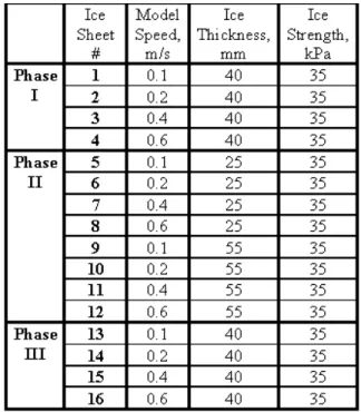
period 1999-2002 and 2002-2005, respectively). One of their main tasks is to develop a procedure for Experimental Uncertainty Analysis (EUA) in ice tank testing. So far, three phases of ship resistance in ice testing have been completed. The test matrix for all three phases is given in Table 1.

The results and analysis from the experiments in Phase III test program are presented in this report. However, for clarity and completeness, a brief summary regarding the previous tow phases is given as follows:

Phase I test program was documented by Derradji-Aouat et al. (2002) and Derradji-Aouat (2002)

in two IOT internal technical reports: The 1st_report

dealt with presenting the experimental program and

test results, while the 2nd_{report dealt with developing a}

methodology to quantify EU in the test results.

The documentation for Phase II test program is also presented in two IOT reports (Derradji-Aouat and Coëffé, 2003, and Derradji-Aouat, 2003). In Phase II, the same test matrix as in Phase I was repeated (Table 1). The only difference is the target thickness of the ice. In Phase I, all tests were conducted for only one target ice thickness (40 mm), while Phase II tests were conducted for two additional ice thicknesses (25 mm and 55 mm). Together, Phases I and II test programs provided information for three different ice thicknesses.

In Phase III, the same test matrix as in Phase I was completed (Table 1). The difference between Phase I and Phase III test programs is that in Phase I, the ship model was attached to the carriage using the tow post (Figure 1a), while in Phase III, the model was attached to the carriage using the PMM (Planar Motion Mechanism, Figure 1b).

(3)

Figure 1a: Ship model in the tow post test setup.

Figure 1b: Ship model in the PMM test setup. All three phases involved experiments in ice and in open water. A total of sixteen (16) different ice sheets were tested. Table 1 gives the nominal ice thickness and the target flexural strength for each sheet. It should be noted that all experiments in ice were very long test runs (the model was towed at constant speed throughout most of the useable length of the ice tank, 76 m). Appendix A provides a summary for Phase III test program.

EXPERIMENTAL UNCERTAINTY ANALYSIS

A literature review for the history and development of EUA in marine/ocean testing facilities was given by Derradji-Aouat (2002).

Mathematically, the EUA procedure presented in this report is based on the equations provided by Coleman and Steel (1998). The latter is in harmony with the guidelines of ISO (1995), ASME (PTC-19.1,

1998), and GUM (2003). The necessary mathematics used to develop an EUA procedure for ice tank testing is given in Appendix B.

SHIP RESISTANCE IN ICE

Since the objective of this paper is to present a procedure for EUA in the results of ship resistance tests in ice tanks, a summary for the standard calculations of ship resistance in ice is given as follows:

The standards for ship resistance in ice (ITTC-4.9-03-03-04.2.1) give the equation for the total resistance in ice as the sum of 4 individual components: ow R b R c R br R t R = + + + (1a)

where Rt is the total resistance, Rbr is the resistance

component due to breaking the ice, Rc is the

component due to clearing the ice, Rb is the component

due to buoyancy of the ice and Row is the resistance

component in open water.

In order to quantify each component, the test plan should include tests in level ice, tests in pre-sawn ice, creeping speed tests, and tests in open water. The

open water tests provide values for Row, while the

creeping speed tests give Rb. In the pre-sawn ice tests,

the ice breaking component Rbr = 0, and therefore:

ow R b R c R t R = + + (1b)

Since Row and Rb are already known (from the

open water and the creeping speed tests), thus:

ow R b R t R c R = − − (1c)

where Rt, in Eq. 1c, is the measured resistance in the

pre-sawn ice test runs.

From tests in level ice, the total resistance Rt

is measured, and the ice breaking component, Rbr, is

calculated as (from Eq. 1a):

ow R b R c R t R br R = − − − (1d)

EUA - PROPOSED PROCEDURE FOR ICE TANK TESTING

The proposed procedure was developed on the basis of one hypothesis and one requirement.

1. Segmentation hypothesis, and 2. Steady state requirement.

(4)

Segmentation Hypothesis

For the test runs in ice, several reasons have contributed to the decision for keeping the speed of the ship model constant throughout most of the useable length of the ice tank (about 65 m – Appendix A). The main one is the hypothesis that the time history from one long ice test run can be divided into segments, and each segment can be analyzed as a statistically independent test. The hypothesis states that:

“The history for a measured parameter (such as tow force versus time) can be divided into 10 (or more) segments, and each segment is analyzed as a statistically independent test. Therefore, the 10 segments in one long test run are regarded as 10 individual (independent but identical) tests.”

Coleman and Steel (1998) reported that, in statistical uncertainty analysis, a population of at least 10 measurements (10 data points) is needed. Uncertainty is calculated using the mean and the standard deviation of that population.

However, in ice tank testing, conducting the same test 10 times is very costly and very time consuming. Therefore, the principle of segmenting a time history of a measured parameter over a long test run into 10 segments, results in significant savings in costs and efforts. In this case, EU are calculated from the means and standard deviations of the individual segments.

In order to further illustrate the segmentation hypothesis, the following example is used (Figure 1a). In this example, the measured tow force history is obtained in test run # 1 (level ice), ice sheet # 2 (nominal ship speed of 0.2 m/s and nominal ice thickness of 40 mm).

The segmentation hypothesis calls for dividing the long time history (Figure 1a) into 10 equal (more or less equal) segments, as illustrated in Figure 1b. Using the tow force segments, the first step is to calculate the mean and standard deviation for each segment. The second step is to calculate the mean of the means and the standard deviation of the means of the segments.

These two steps of calculations are repeated for all test runs in ice (continuous, pre-sawn and broken ice test runs, all six test runs, Appendix A )

It should be cautioned that the segmentation hypothesis is valid only if the following 3 conditions are satisfied (Derradji-Aouat, 2004):

1. Each segment should span over 1.5 to 2.5 times the length of the ship model,

2. Each segment should include at least 10 events for ice breaking (10 ice load peaks) or at least 10 collision events (in case of pack ice test runs), and 3. General trends (of a measured parameter such as

tow force versus time) are repeated in each segment.

Condition # 1 is based on the fact that the ITTC procedure for resistance tests in level ice (ITTC-4.9-03-03-04.2.1) requires that a test run should span over at least 1.5 times the model length. For high model speeds (> 1 m/s), however, the ITTC procedure requires test spans of 2.5 times the model length. Condition # 2 is based on the fact that in EUA, for an independent test, a population of at least 10 data points is needed to achieve the minimum value for the factor t (Eq. B.2 - Appendix B). The gain in any further reduction in the value of t, by having more than 10 segments, is minimum (Derradji-Aouat, 2003).

Condition # 3 is introduced to ensure that the overall trends in a measurement are repeated in each segment. This condition serves to provide further assurance into the main hypothesis (“…the 10 segments in one long test run are regarded as 10 individual, independent but identical, tests”). Fundamentally, if the trends are not, reasonably, repeated, then the segments could not be analyzed as “independent but identical” tests.

Table 1: Test matrix.

(5)

PICE-2, Run 1, V = 0.2m/s -50 0 50 100 150 200 90 140 190 _{Tim e (s)} 240 290 340 To w Fo rc e (N )

Figure 2a: Example for a measured tow force history (PICE-2 refers to ice sheet #2).

Segment 4 -40 0 40 80 120 90 100 Time (s) 110 120 Tow Forc e (N) Segment 5 -50 0 50 100 150 200 110 120 Time (s) 130 140 Tow Force ( N ) Segment 6 -50 0 50 100 150 140 150 Time (s)160 170 Tow For ce (N) Segment 7 -50 0 50 100 150 170 180 Time (s) 190 200 Tow For ce (N) Segment 8 -50 0 50 100 150 190 200Time (s)210 220 230 Tow Forc e (N) Segment 9 -50 0 50 100 150 220 230 Time (s)240 250 Tow For ce (N) Segment 10 -50 0 50 100 150 250 260 Time (s) 270 280 Tow For ce (N) Segment 11 -50 0 50 100 150 200 280 290 Time (s) 300 310 Tow For ce (N) Segment 12 -50 0 50 100 150 200 305 315 Time (s) 325 335 Tow Forc e ( N ) Segment 13 -50 0 50 100 150 200 335 345 Time (s) 355 365 Tow For ce (N)

Figure 2b: Division of the tow force time history (in Figure 2a) into segments.

(6)

The time histories measured in creeping speed tests are not subjected to the segmentation hypothesis. Furthermore, it is recognized that the division of the results of a test run into segments is valid only for the steady state portion of the measured data (only the steady state portion of the measured time history is to used for the segmentation). This is required to eliminate the effects of the initial ship penetration into the ice (transient stage) and the effects of the slowdown and full stop of the carriage during the final stages of the test run (also transient stage).

Steady State Requirement

In ice tank testing, for any given ice sheet, the ice properties are not completely (100%) uniform (same thickness) and homogeneous (same mechanical properties) all over the ice sheet. This is attributed, mainly, to the ice growing processes and refrigeration system in the ice tank. Figure 3 shows examples for “measured spatial variability” of ice thickness and flexural strength of an actual ice sheet in the tank.

Figure 3a: Measured 3-D profiles of typical spatial variation of ice thickness in the tank.

In addition to the spatial variability of the material properties of ice, during an ice test run, the carriage speed may (or may not) be maintained at exactly the required nominal constant speed. The control system maintains the carriage speed constant. However, when ice breaks, small fluctuations in carriage speed may take place.

Because of this inherent non-uniformity of ice sheets, the non-homogeneity of ice properties and the small fluctuations in the carriage speed, steady state in the time history of a measurement may not be achieved. For example, in Figure 1a, the tow force did not become completely steady after the initial transient stage.

Theoretically, if the time history of a measured parameter is changing drastically, then the segments could not be analyzed as “identical” tests. The steady state requirement, therefore, calls for a corrective action to account for the effects of non-uniform ice thickness, non-homogenous ice mechanical properties and small fluctuations in

carriage speed on the test measurements.

Figure 3b: Measured 3-D profiles of typical spatial variation of the flexural strength of ice in the tank.

To identify whether or not the time history for a measured parameter has reached its steady state, the following procedure was recommended. The time histories for the measured parameters, in all ice test runs, were plotted along with their linear trend lines (Derradji-Aouat and van Thiel, 2004). A linear trend line with zero slope (or very close to zero) indicates that a steady state in a measured parameter is achieved. After drawing the linear trend lines through all measured tow forces, it was observed that, in the majority of cases, a true steady state was never achieved. For example, the linear trend lines show that the tow force time histories sloped over a range of 0.002% (ice sheet # 2, Run #3) to 5.2% (ice sheet # 4, Run #1). Derradji and van Thiel (2004) showed that, although the slopes of the trend lines varied within only 5.2%, they led to some significant changes in the magnitude of tow forces over the 65 m towing distance. They suggested that the non-steady state condition may be attributed to one (or all) of the following 3 factors:

1. A changing carriage speed (or small fluctuations in carriage speed) during testing,

2. Non-uniform ice thickness,

3. Non-uniform mechanical properties of the ice (flexural/compressive strengths, elastic modulus, density of ice, …).

(7)

The contribution of each factor was investigated by Derradji Aouat and van Thiel (2004), and they concluded that the effect of changing carriage speed can be ignored (that is factor # 1). The effects of the other two factors are given as:

NON-UNIFORM ICE THICKNESS

Mean ice thickness profiles were calculated, each mean profile is the average of 3 measured ice thickness profiles (along the CC, NQP and SQP). Each profile is a series of ice thickness measurements (every 2 m) along the length of the ice tank.

The linear trend lines, through the mean profiles, indicate that the ice thickness varied within a range of 0.69% to 2.64%.

To correct for the effects of non-uniform ice thickness on the two force measurements, the following correction methodology and rational were followed (Derradji-Aouat, 2002):

Note that, in this forgoing discussion, mean ice resistance values are used to show how the EUA method is conceptualized and developed. The same correction methodology are used for maximum ice resistance values (Derradji-Aouat, 2002). Also, note that ice thickness corrections are applied only to the resistance due to the ice. Therefore, the total ice

resistance (RTotal Ice) is equal to the measured resistance

in the ice tests (RMeasured) minus the resistance measured

in the baseline open water tests (ROpen Water).

(

RTotal Ice

)

Mean =

(

RMeasured

)

Mean−

(

ROpen Water

)

(2a)

The value of (ROpen Water) is obtained from the

correlation obtained from the baseline open water test results (Appendix A).

For a given ice sheet, with nominal thickness ho, the following equation is used to correct for the total ice resistance (Derradji-Aouat, 2003):

(

)

(

)

h

*

R

m o Mean Measured Ice Total Mean Correct Ice Total



_









=

(2b)

where (RTotal Ice) Correct Mean is the corrected total ice

resistance, (RTotal Ice) Measured Mean is the measured total

ice resistance, ho is the nominal ice thickness (40 mm),

and the hm is the measured ice thickness at a distance D

(D is the distance in the tank where hm .is measured,

Derradji-Aouat and van Thiel, 2004).

Note that only the results of tests in continuous ice (Run # 1, # 2 and # 3) are subjected to ice thickness corrections. In broken ice test results (Run # 4, # 5 and # 6), no corrections were necessary. This stems from the fact that, in broken ice tests, the original ice thickness profiles are not maintained.

The time histories measured in the creeping speed test runs are also not subjected to corrections for ice thickness variation. The length of each creeping speed test run is small (only one ship length ≈ 3.8 m), the variation of ice thickness over this small length can be ignored.

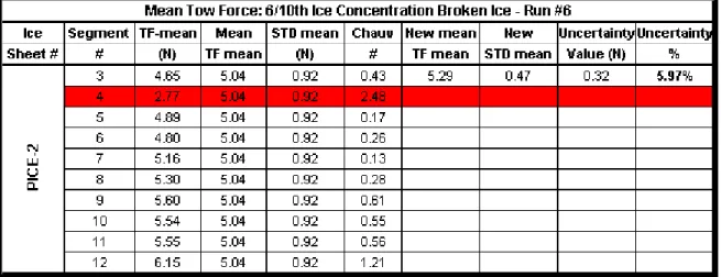
Table 2: Example for calculations of random uncertainties in mean tow forces (Ice Sheet # 2, Run # 6, Model speed = 0.2 m/s)

(8)

NON-HOMOGENEOUS ICE PROPERTIES

Mean flexural strength profiles along the length of the ice tank were given by Derradji-Aouat and van Thiel (2004). In each ice sheet, two flexural strength profiles along the SQP and NQP are measured every 15 m.

The flexural strength profiles are obtained using in-situ cantilever beam tests. The beam dimensions have the proportions of 1:2:5 (thickness,

hf,: width, w: length, L). The flexural strength σf is

calculated as: 2

6

f f

wh

PL

=

σ

(3a)

where P is the point load.

The uncertainty in the flexural strength is Uσf:

2 hf 2 W 2 L 2 P f

U

2 U

U

σ

=

+

(3b)

where UL, UW, and Uhf are the uncertainties in the

measured dimensions (L, W and hf). Up is the

uncertainty in the measured point load.

The uncertainties in the flexural strength profiles are calculated using Eq. 3b. Derradji-Aouat (2002) reported that any data correction for ice thickness includes, implicitly, the correction for the flexural strength of the ice. This is due to the fact that ice thickness is a fundamental measurement while the flexural strength is a calculated material property (flexural strength is calculated from measurements of applied point load and dimensions of the ice cantilever beam). Since this work deals with EUA of actual “fundamental” measurements, it is recognized that if corrections were to be made for both ice thickness and flexural strength, double correction (double counting) would take place, and the final uncertainty values would be overestimated. The same argument is valid for corrections for the comprehensive strength of ice (the latter is calculated from applied axial load and measurements of actual dimensions of the ice sample).

Measured ice density profiles along the length of the ice tank were also given by Derradji-Aouat and

van Thiel (2004). The density of ice, ρi, is given as:

V M

w

i =

ρ

−

ρ

(4a)

where ρw is the density of water. M is the mass of the

ice sample. The volume, V, is calculated from the sample dimensions (length, L, width, W, and thickness, H): The uncertainty in the ice density is:

2 M 2 W 2 L 2 H i ρ

U

=

+

(4b)

The variation of density along the centre line of the tank was between 4.58% to 8.60%. To a large extent, this range is a reflection of the uniformity of non-bubbly ice. From the ice tank operational point of view, in non-bubbly ice sheets, density value could not be controlled but its uniformity is reasonably assured. In bubbly ice, however, the inverse is true, the target density values can be achieved in pre-set locations in the tank but its spatial uniformity is compromised.

CALCULATIONS RANDOM UNCERTAINTIES

In the following example, the discussion will be focused on the mean tow force history (Figures 1a and 1b). Table 2 shows the segments for the mean tow force history obtained in ice sheet # 2 for Run #6. Essentially, the tow force history is divided into 10

segments. Mean tow force (TFMean) is obtained for each

segment.

The mean of the 10 means (Mean_TFMean) and

the standard deviation of the 10 means (STD_TFMean)

were calculated (as shown in Table 2). Random

uncertainties in the tow forces U(TFMean) are calculated

in three steps:

Step # 1: In Table 2, after the calculations of the mean of means and standard deviation of means, the Chauvenet’s criterion is applied to identify outliers (outliers are discarded data points). The Chauvenet

number for mean tow forces is (Chauv #)Mean:

(

)

(

)

STD_TF Mean_TF - TF Chauv # Mean Mean Mean Mean       = (5a)

For 10 to 15 segments, the Chauv # should not exceed 1.96 to 2.13. In Table 2, data points with Chauv # greater than 1.96 were disregarded (shaded cells). A new mean of means and a new standard deviation of means are calculated from the remaining data points (remaining segments).

(9)

Run #1: Mean Tow Force in Level Ice 0 10 20 30 40 50 60

PICE-1 PICE-2 PICE-3 PICE-4

Ice Sheet

M

ean Tow Force (N

)

Run #2: Mean Tow Force in Presawn Ice

0 5 10 15 20 25 30 35

Ice Sheet

Mean Tow For

ce (

N

)

Run #3: Mean Tow Force in Unsupported Ice

0 10 20 30 40 50

Ice Sheet

Mean Tow For

ce (N)

Run #4: Mean Tow Force in 9/10th Ice Concentration 0 3 6 9 12 15 18

Ice Sheet M e a n Tow Forc e (N)

Run #5: Mean Tow Force in 8/10th Ice Concentration 0 3 6 9 12 15 18

Ice Sheet

Mean Tow For

ce (N)

Run #6: Mean Tow Force in 6/10th Ice Concentration

0 5 10 15

Ice Sheet

Mean Tow For

ce (

N

)

Figure 4a Measured mean tow forces presented as function of the ice sheet number.

Step # 2: After calculating the new mean of the means and the new standard deviation of the means (from the remaining segments - data points), random uncertainty in the mean tow force is:

(

)

N STD_TF t*

)

U(TFMean _= Mean

      (5b)

where t ≈ 2, and N is the number of the remaining data points (valid segments).

Step # 3: Random uncertainties (Eq. 5b), are expressed in terms of uncertainty percentage (UP):

100 * Mean_TF ) U(TF ) UP(TF Mean Mean Mean _=       (5c)

Note that the above three steps are also used to calculate random uncertainties in maximum tow forces. This is achieved by substituting the subscript “mean” by the subscript “max” in Eqs. 5a, 5b and 5c.

(10)

Run #1: Uncertainty in Level Ice 0% 1% 2% 3% 4% 5%

Ice Sheet

U

M

ean Tow Force (%)

Run #2: Uncertainty in Presawn Ice

0% 1% 2% 3% 4% 5% 6% 7%

Ice Sheet

U Mean Tow Force (%)

Run #3: Uncertainty in Unsupported Ice

0% 1% 2% 3% 4% 5% 6%

Ice Sheet

U

M

ean Tow Force (%)

Run #4: Uncertainty in 9/10th Ice Concentration

0% 3% 6% 9%

Ice Sheet

U Mean Tow

Force (%)

0% 5% 10% 15% 20% 25% 30%

Ice Sheet

U Mean Tow

Force (%)

0% 2% 4% 6% 8% 10% 12% 14%

Ice Sheet

U Mean Tow

Force (%)

Figure 4b: Uncertainties in mean tow forces presented as function of the ice sheet number.

It is important to note that the above procedure (segmentation of measured time history, check for the steady state requirement, correction for ice thickness, the use of the three calculation steps) is valid for calculating random uncertainties in all other measured ship motion parameters (such as pitch, heave, yaw and sway).

RANDOM EU IN MEAN TOW FORCES

Figures 4a and 4b show the measured mean tow forces and their random uncertainties (calculated using the above steps). The figures show that:

In level (continuous, unbroken) ice test runs (Run # 1, # 2 and # 3), calculated random uncertainties in mean tow forces are less than 6%. In fact, all uncertainties were below 4%, except for two data points (ice sheet #1, Run #2 and ice sheet # 4, Run #3), where uncertainties values were 5.84% and 4.08%, respectively.

In broken ice test runs (Run # 4, # 5 and # 6), all random uncertainties were below 18%, except for test run # 5 in ice sheet # 1, where the uncertainty value was 25.94 %. It should be emphasized that in broken ice tests, no corrections for ice thickness profiles were made.

(11)

EFFECTS OF DATA REDUCTION EQUATIONS

Equation 2b was proposed to correct for the effects of ice thickness variations on the values of random uncertainties. It should be recognized that the corrected resistance curves are not direct laboratory measurements, but they are calculated from the analytical Eq. 2b. The process of using analytical equations to correct measured parameters is called “Application of Data Reduction Equations, DRE”.

In EUA, there are additional random uncertainties involved in the application of the DRE. The uncertainty involved in using Eq. 2b is:

h U R UR R UR 2 1 2 2 0 h 0 0               +       =       ₍₆₎

In the above equation, (UR/R) is the total

uncertainty in resistance, R. Both (UR0/R0) and (Uh/h0) are the relative uncertainty in the measured ice resistance (as shown in the example in Table 2) and the relative uncertainty in the measured ice thickness,

respectively. Note that, in Eq. 6, the value of (Uh/h0) is

an additional relative uncertainty, which is induced by the use and application of the DRE. The total uncertainty is the geometric sum of both relative uncertainties (UR0/R0) and (Uh/h0).

COMPARISON OF UNCERTAINTY VALUES IN CONTINUOUS ICE AND IN PACK ICE TESTS.

In continuous ice (including presawn ice sheets), random uncertainties were mainly under 6%. However, in broken ice tests, uncertainties of up to 18% were obtained (except in 2 cases). The value of 18% is higher than in continuous ice (6%). The difference between the two uncertainties is attributed to several factors (the details were given by Derradji-Aouat, 2002).

COMPARISON OF UNCERTAINTY VALUES IN MEAN AND IN MAXIMUM TOW FORCES

Figure 5 shows comparisons between random uncertainties in mean tow forces and those in maximum tow forces. In general, uncertainties in maximum tow forces are higher than those in mean tow forces (ration of 2 to 4). The details were given by Derradji-Aouat and van Thiel (2004).

Examples for omparisons among the results of all three phases of testing are given in Figures 6a and 6b.

CONCLUSIONS AND RECOMMENDATIONS

In continuous ice test runs, the uncertainty range of 3% to 10% was obtained (in all three phases). This is consistent with the range of uncertainties obtained in Phases I and II test programs. This is also consistent with the previously reported studies (in the literature) using different ship models, in different ice tanks, in different countries over a time span of 10 to 12 years (Appendix B).

In broken ice, the uncertainties ranged from to 3% to 26%. This is also consistent with the calculated range in Phases I and II test programs. In pack ice conditions, large uncertainties are possible (and sometimes expected) in randomly broken ice.

Comparison between uncertainty in maximum and mean tow force

0% 5% 10% 15% 20% 25% 30% 0% 5% 10% 15% 20% 25% 30% Uncertainty in Mean Tow Force (%)

Uncertai n ty i n M ax Tow Force (% ) Run #1 Run #2 Run #3 Run #4 Run #5 Run #6

Figure 5: Comparison of uncertainties in measured mean tow force with those in maximum tow force.

REFERENCES

ASME PTC 19.1-1998, “Test Uncertainty. Supplement to Performance Test Code, Instruments and Apparatus”.

Coleman H.W. and Steele W.G., “Experimentation and

Uncertainty Analysis for Engineers”, 2nd edition, John

Wiley & Sons publications, New York, 1998.

Derradji-Aouat A., Moores C. and Stuckless S., “Terry Fox Resistance Tests. The ITTC Experimental Uncertainty Analysis Initiative”, IMD report # TR-2002-01.

Derradji-Aouat A., “Experimental uncertainty analysis for ice tank ship resistance experiments”, IMD/NRC report # TR-2002-04.

Derradji-Aouat A. and Coëffé J., “Terry Fox Resistance Tests – Phase II. The ITTC Experimental Uncertainty Analysis”, IMD report # TR-2003-07.

(12)

Speed = 0.1 m/s : Compare P1 & P3 Mean Tow Force 0 10 20 30 40 50

Run #1 Run #2 Run #3 Run #4 Run #5 Run #6

M e a n Tow Forc e (N )

Phase 1: Tow Post Phase 3: PMM

Speed = 0.2 m/s: Compare P1 & P3 Mean Tow Force

0 10 20 30 40 50

Speed = 0.4 m/s: Compare P1 & P3 Mean Tow Force

0 10 20 30 40 50 60

Speed = 0.6 m/s: compare P1 & P3 Mean Tow Force

0 15 30 45 60 75

Figure 6a: Comparison of test results: Measured mean tow forces using the tow post (Phase I) and measured mean tow forces using the PMM (Phase III).

Derradji-Aouat A. “Phase II Experimental uncertainty analysis for ice tank ship resistance experiments”, IMD/NRC report # TR-2003-09.

Derradji-Aouat A and van Thiel A., “Terry Fox Resistance Tests – Phase III (PMM Testing). The ITTC experimental uncertainty analysis initiative”, IOT/NRC report # TR-2004-05.

Derradji-Aouat A.. “A Method for Calculations of Uncertainty in Ice Tank Ship Resistance Testing”,

Proceedings of the 19th International Symposium on

Sea Ice, 2004, PP. 196-206, Mombetsu, Japan.

GUM., General Uncertainty Measurements, 2002 (http://www.gum.dk/)

ISO., “Guide to the Expression of Uncertainty in Measurements”, 1995, .ISBN 92-67-10188

APPENDIX A:

TEST PROGRAM AND TEST RESULTS

In phase III test program, the main components of the test set up are: The Terry Fox ship model, the Planar Motion Mechanism (PMM), data acquisition system (DAS) and video cameras.

This phase of testing required 4 different ice sheets. All ice sheets were made up of non-bubbly ice, they all have the same target thickness (40 mm) and the same target flexural strength (35 kPa). Preparing the ice tank, seeding and growing the ice sheets, surveying for the mechanical properties of ice (flexural and comprehensive strengths, elastic modulus and density) and ice thickness profiles were performed as per the IOT internal standards and work procedures, which are similar to the ITTC recommended procedures.

Two types of experiments were performed: Experiments in ice and experiments in open water.

(13)

PICE-1: Compare P1 & P3 Uncertainty in Mean Tow Force at 0.1m/s

0% 5% 10% 15% 20% 25% 30% 35%

U

(%)

M

ean Tow

Force Phase 1: Tow Post Phase 3: PMM

0% 5% 10% 15% 20% 25%

U

(%)

M

ean Tow

Force

0% 4% 8% 12% 16% 20%

U

(%)

M

ean Tow

Force Phase 1: Tow Post Phase 3: PMM

0% 2% 4% 6% 8% 10% 12% 14%

U

(%)

M

ean Tow

Force

Figure 6b: Comparison of uncertainties in mean tow force using the tow post (Phase I) and the PMM (Phase III). The experiments in ice involved:

1.a: Experiments in level ice sheets (unbroken).

1.b: Experiments in pre-sawn ice sheets.

1.c: Experiments in pack ice (broken)

The experiments in open water involved:

2.a: Standard resistance experiments in open water

(as per the ITTC procedure)

2.b: Baseline experiments in open water (constant

speed through the length of the tank)

Figure A.1a: Terry Fox model on the calibration frame in the fabrication shop:

Figure A.1b: Terry Fox model on the shop floor (model is in its storage wooden cradle). Length at water level is 3.74 m, Maximum beam at water level is 0.79 m, Model scale is 1/20.8

(14)

EXPERIMENTS IN ICE

Ship model speeds of 0.1 m/s, 0.2 m/s, 0.4 m/s, and 0.6 m/s were selected. Each ice sheet was tested for only one speed. For example, ice sheet #1 was tested for speed of 0.1 m/s, ice sheet # 2 was tested for speed 0.2 m/s. In each ice sheet, six (6) different test runs were performed. The first three runs were conducted in level and pre- sawn ice sheets, while the last three runs were conducted in pack “broken” ice. A total of 24 resistance test runs in ice were performed.

A schematics for the six (6) ice test runs is shown in Figure A.2. The first three test runs are: • Run # 1: This run was performed in level ice,

along the centerline of the tank (the central channel, CC). The carriage speed was kept constant along the entire useable length of the ice tank (~ 65 m). Note that after the completion of this run, an open water channel along the centerline of the tank is created.

•

• • •

Run # 2: The model was moved to the South Quarter Point (SQP) of the tank. The south half of the ice sheet was constrained (using pegs), and the ice was pre-sawn along the SQP straight path. Resistance test run was performed in the pre-sawn ice at constant speed (same speed as Run # 1). Run # 3: The model was moved to the North Quarter Point (NQP) of the tank. The north half of the ice sheet was neither pre-sawn nor constrained. Resistance test run was performed in the ice sheet at constant speed (same speed as Run # 1).

Runs # 4, # 5, and # 6 were performed in pack (broken) ice. After the completion of the first 3 runs, the ice sheet was broken (manually) into small blocks (about 300 mm X 300 mm). Then, the blocks were redistributed in the tank, manually, to achieve the desired pack ice concentration. Three (3) different ice concentrations were targeted. These are:

Run # 4: Test run in 9/10ths_{ice concentration, tow}

along the NQP at a constant speed.

along the CC at a constant speed.

along the SQP at a constant speed.

These ice concentrations were chosen to reflect actual pack ice environment. Ice concentration less than about 6/10 yields a behaviour equivalent to that of baseline open water tests. Figure A.3 is

Figure A.2: A schematic for Run # 1, # 2 and # 3

Figure A.3: Typical test run in broken ice (Phase III) Free Boundary Tests Run # 3 12 m SQP NQP CC 76 m Constrained Boundary Pre-Sawn Ice Test Run # 2 Test Run # 1

(15)

Tow Force versus Velocity: Phase 1, 2 & 3 Open Water Baseline Resistance Tests

y = 19.091x2_{+ 1.3155x + 0.0388} R2_{= 0.9959} 0 1 2 3 4 5 6 7 8 9 0 0.1 0.2 0.3 0.4 0.5 0.6 0.7 Velocity (m/s) Tow Force (N)

Phase III: Tow Force vs. Velocity in Continuous Ice

0 10 20 30 40 50 60 0 0.1 0.2 0.3 0.4 0.5 0.6 0.7 Velocity (m/s) Tow For ce (N)

Level Ice (Run #1) Pre-sawn Ice (Run #2) Unsupported Ice (Run #3)

Figure A.4a: Baseline open water tests (best fit for all three phases of testing).

Figure A.4b: Standard open water tests (best fit for all three phases of testing).

EXPERIMENTS IN OPEN WATER

Standard Resistance Experiments in Open Water: A series of standard resistance tests in open water were performed in the ice tank (calm water). In all tests, turbulent stimulation studs were placed on the model and beach absorbers were used. Ship speeds from 0.1 m/s to 1.8 m/s were covered (increments of 0.2 m/s). Baseline Resistance Experiments in Open Water: In this series of tests, the turbulent studs and beach absorbers were removed. In each test, model was towed in calm open water at constant velocity along the entire useable length of the ice tank (~ 65 m). Velocities of 0.1 m/s, 0.2 m/s, 0.4 m/s and 0.6 m/s were tested.

TEST RESULTS

Figures A.4a and A.4b show the results from the standard open water resistance tests and the results from the baseline open water tests, respectively.

Figure A.5a: Measured Tow Force in Continuous Ice.

Figure A5b: Measured Tow Force in Broken Ice Figures A.5a and A.5b give the results for the test runs in ice. Best fit curves through the data are provided. As expected, the results are typical of resistance data of a ship such as the Terry Fox in ice. Detailed presentation of the test program and test results were given in an internal report by Derradji-Aouat and van Thiel (2004). The results for the surveys for the flexural and compressive strengths, elastic modulus and ice density were also included in the report.

APPENDIX B:

BASIC FORMULATION

In a typical experiment, the “total uncertainty, U” is the sum of a “bias uncertainty, B” and a “random uncertainty, P”. Bias uncertainties (also called systematic uncertainties) are due to uncertainty sources such as load cell calibrations, accuracy of motion instrumentations and DAS. Random uncertainties (also called precision or repeatability uncertainties) are a

Tow Force versus Velocity: Phases 1, 2 & 3 Open Water Standard Resistance Tests

y = 32.21x2_{- 11.354x} R2_{= 0.9735} 0 10 20 30 40 50 60 70 80 90 0 0.2 0.4 0.6 0.8 1 1.2 1.4 1.6 1.8 Velocity (m/s) Tow Force (N)

Phase III: Tow Force vs. Velocity in Broken Ice

0 4 8 12 16 20 0 0.1 0.2 0.3 0.4 0.5 0.6 0.7 Velocity (m/s) Tow Forc e (N)

9/10th ice concentration (Run #4) 8/10th ice concentration (Run #5) 6/10th ice concentration (Run #6)

(16)

measure of the degree of repeatability in the test results (i.e. if a test was to be repeated several times, would the same results be obtained each time?). Examples for random uncertainty sources are the changing test environment (such as fluctuations in room temperature during testing), small misalignments in the initial test setup, human factors, …etc.

Mathematically, the total uncertainty is:

(

B

P

)

U

₌

_±

2

₊

2 (B.1) For a single test population (where only one test is performed, and for that one test, N data readings are obtained), random uncertainty “P” from an uncertainty source “X” is Px:

S

*

t

P

X X

=

(B.2a)

The coefficient “t” is obtained from the standard table for a normal Gaussian distribution. Its value depends on the desired level of confidence (usually, 90% to 95%) and the number of the Degree of Freedom (DOF) in the sample population. The DOF = N –1, where N is the numbers of data readings. For DOF ≥ 10, t ≈ 2.

In a multi-test population (where the same test is repeated N times, and each test is represented by only one data point in the population of N data points), the random uncertainty from an uncertainty source “X” is PNX:

N

S

*

t

P

NX NX

=

(B.2b)

Derradji-Aouat (2002) showed that in a typical ice tank ship resistance test, the bias uncertainty component (B) is much smaller than the random one (P), he reported that, in Phase I ship model tests in ice, the value of (B) is at least one order of magnitude smaller than the value of (P). He concluded, therefore, that; in routine ship resistance ice tank testing, the total uncertainty (U) can be taken as equal to the random one. Simply, without a loss of accuracy, the bias uncertainty component can be neglected. It follows that:

P

U

=

±

(B.3)

The above equations are valid for direct measurements (directly measured variables, such as load, deformation, motion, pitch, roll, …etc.). In most cases, the measured variables are used to compute engineering parameters (such as stress, strain, resistance, …etc.) using Data Reduction Equations (DRE). Additional uncertainties due to the use of DRE need to be considered (as discussed in the paper).

REVIEW - EUA IN ICE TANK TESTING

Newbury (1992) conducted several standard ship resistance tests in ice, at the NRC/IMD ice tank, using a model fo

r R-class icebreaker. He used nine (9) ice sheets to execute the test program. Of the 9 ice sheets, five (5) ice sheets had nominal thickness of about 35 mm and flexural strength of about 40 kPa, two (2) ice sheets had nominal thickness of about 50 mm and flexural strength of about 40 kPa, and two (2) ice sheets had nominal thickness of about 22.5 mm and flexural strengths of about 40 kPa and 20 kPa, respectively. The tests were conducted for various model speeds (ranging from 0.15 m/s to 0.9 m/s).

In each test, Newbury (1992) calculated the mean and standard deviation for ice breaking resistance. In most tests, his calculations showed that the ratio of the standard deviation to the mean resistance was within 5%; expect for 2 cases, where the ratios were 8.7% and 11.8 %, respectively. If uncertainties were to be calculated using Eq. B.2, Newbury’s (1992) test results show that random uncertainties in ice breaking resistance would be about 10% to 12%. In the extreme two cases, random uncertainties will be about 18 % to 22%. Note that random uncertainty range of 10% to 12% is, more or less, supported and confirmed by Kitagawa et al. (1991 and 1993).

Kitagawa et al. (1991 and 1993) published ice breaking resistance data obtained in the ice tank of National Maritime Research Institute of Japan (NMRI). Total uncertainties of about 10% were calculated (in some cases, uncertainties of about 20% were reported).

Figure A6: Actual ice braking operations off the coast of Newfoundland and Labrador, Canada.