Publisher’s version / Version de l'éditeur:
Acta Acustica, 89, Jan-Feb 1, pp. 110-122, 2003-01-01
READ THESE TERMS AND CONDITIONS CAREFULLY BEFORE USING THIS WEBSITE.
https://nrc-publications.canada.ca/eng/copyright
Vous avez des questions? Nous pouvons vous aider. Pour communiquer directement avec un auteur, consultez la
première page de la revue dans laquelle son article a été publié afin de trouver ses coordonnées. Si vous n’arrivez pas à les repérer, communiquez avec nous à [email protected].
Questions? Contact the NRC Publications Archive team at
[email protected]. If you wish to email the authors directly, please see the first page of the publication for their contact information.
Archives des publications du CNRC
This publication could be one of several versions: author’s original, accepted manuscript or the publisher’s version. / La version de cette publication peut être l’une des suivantes : la version prépublication de l’auteur, la version acceptée du manuscrit ou la version de l’éditeur.
Access and use of this website and the material on it are subject to the Terms and Conditions set forth at
Expressions for first-order flanking paths in homogeneous isotropic
and lightly damped buildings
Nightingale, T. R. T.; Bosmans, I.
https://publications-cnrc.canada.ca/fra/droits
L’accès à ce site Web et l’utilisation de son contenu sont assujettis aux conditions présentées dans le site LISEZ CES CONDITIONS ATTENTIVEMENT AVANT D’UTILISER CE SITE WEB.
NRC Publications Record / Notice d'Archives des publications de CNRC:
https://nrc-publications.canada.ca/eng/view/object/?id=483735e7-d070-41c7-ab50-2d8376b037d3 https://publications-cnrc.canada.ca/fra/voir/objet/?id=483735e7-d070-41c7-ab50-2d8376b037d3
Expressions for first-order flanking paths in
homogeneous isotropic and lightly damped buildings
Nightingale, T.R.T.; Bosmans, I.
NRCC-45376
A version of this document is published in / Une version de ce document se trouve dans :
Acta Acustica, v. 89, no. 1, Jan-Feb. 2003, pp. 110-122
Expressions for first-order flanking paths in homogeneous
isotropic and lightly damped buildings
TRT Nightingale, National Research Council Canada, Institute for Research in Construction, Building M27 1200 Montreal Road, Ottawa, Ontario Canada K1A 0R6
and
I Bosmans, LMS International, Engineering Services Division, Interleuvenlaan 68, B-3001 Leuven, Belgium
Summary
Expressions for first and second-order flanking paths are derived using the framework and assumptions of Statistical Energy Analysis (SEA). The resulting expression can be rewritten in terms of the sound reduction index (SRI) for resonant transmission through the structural flanking elements and it is shown that consideration must be given to the presence of a non-resonant component in measured SRI. Failure to do so will underestimate the SRI of the flanking paths. The SEA expression for first-order flanking paths is shown to be identical to the expression appearing in EN12354 Part 1 for airborne sound insulation, even though EN12354 was not derived using SEA. To help define situations for which the expressions are valid a set of criteria are presented and discussed.
PACS: 43.55.p 1. Introduction
Recently, there has been considerable effort devoted to the creation and standardisation of a suite of building acoustics prediction models applicable to heavy monolithic constructions. The result is the EN12354 series with Parts 1 and 2 addressing airborne1 and impact2 sound insulation, respectively. These standard models are based on the earlier work of Gerretsen3,4 who created expressions for first-order flanking paths in terms of the sound reduction of the flanking elements and the velocity attenuation at the junction between the building elements in the source and receive rooms. A first-order flanking path is a transmission path from the source to receiver room that involves a single building element in the source room, a single element in the receiver room and a single junction connecting them. Because the expressions formulated by Gerretsen, and those of EN12354, were not derived using a formalised modelling framework such as SEA or FEM, the underlying assumptions and the possible limitations may not be fully appreciated or understood by many users.
This paper shows that the EN12354 expressions for first-order flanking paths can be derived using the SEA framework. A set of applicability criteria based on the requirements for SEA subsystems are given to help practitioners assess the suitability of EN12354 (and SEA) for a particular situation and includes a brief discussion of bias errors. Two appendixes focus on methods to minimise two of the more prominent sources of bias. Appendix A considers the possible bias introduced in EN12354 when the measured data are used to estimate the
resonant sound reduction index of flanking elements. The expression derived in the appendix can be used to estimate the bias and can also be used to correct for the non-resonant component present in measured data. Appendix B derives an expression for second-order flanking paths in terms of EN12354 input data to show that EN12354 can not be extended to higher orders simply by summing the junction attenuation terms (Kij’s).
The paper begins with a brief review of SEA and its application to buildings. A thorough treatment of the subject is available elsewhere5.
2. Introduction to SEA and Subsystems in Buildings
SEA is a modelling framework based on theory derived for weakly coupled oscillators where at steady state the power flow between acoustically coupled systems is determined by the difference in the stored modal energies and the net power supplied to a system is equal to the power dissipated by that system. The concept of a resonant oscillator storing energy has been generalised through the definition of a “subsystem.” For a building it might be a room, wall, floor, or other building element supporting a group of modes with similar properties and energies. Most homogeneous, isotropic and moderately damped building elements and rooms can be considered as being individual subsystems. In this paper each subsystem is given a unique number which is used to allow flanking path identification as well as to indicate to which subsystem a parameter is referring.
Ideally each building element modelled as a subsystem would exhibit the properties of an ideal SEA subsystem, namely:
a.) Support resonant modes of vibration in the frequency range of interest; b.) Vibration response controlled by resonant modes of vibration;
c.) Uniform energy density (by virtue of a reasonably diffuse field); d.) Weakly coupled to other subsystems;
e.) Moderately damped.
In reality most subsystems only approximate these conditions and the accuracy of the SEA prediction is usually determined by the closeness with which the subsystems approximate these conditions.
Several types of building constructions or elements will not satisfy these conditions. They include walls or floors with large ribs or attached stiffeners, especially ones located at equally spaced intervals6. These require special treatment. Highly damped structures7, such as wood framed walls and floors8 where often there is a strong gradient in the energy density and the direct field from the source dominates, also require special treatment. The simple SEA presented in this paper is not appropriate for these types of elements as they can not be considered as single subsystems. In this paper, it is assumed that the elements (subsystems) are homogeneous and isotropic.
Small elements, which do not support modes at the lowest frequency of interest, should not be considered as a subsystem. An example might be a narrow section of wall connecting and offsetting two other walls. Elements like these are usually treated as a part of the junction rather than separate subsystems.
There is also the danger that large elements are mistakenly treated as two subsystems because of construction geometry rather than the physical response of the elements. An example might be a continuous concrete slab under a partition wall. If the wall is either very much lighter than the floor slab, or is very lightly coupled to the floor (caused by the presence of an interlayer or a few point connections), then it is quite likely that the vibration response of the floor slab will be unaffected by the presence of the wall. In this case, when considering the floor-floor flanking path, the floor should be modelled as a single subsystem. When the building has been divided into appropriately chosen subsystems and models developed for the various junctions then the agreement between measured and predicted sound insulation can be quite good5. Fortunately, criteria are available to help in the selection of subsystems and to assess the suitability of SEA. These are discussed in more detail Section 4.
It must be recognised that in addition to first-order flanking paths there will be higher order flanking paths that will also contribute to transmission from the source to receiver room. Thus, limiting the paths to first-order bending will underestimate the transmission and will overestimate the apparent sound reduction index between the rooms. The magnitude of this bias error is a complex function of the number of rooms forming the building and geometry, the construction type, as well as the damping. Recent theoretical work9 has indicated that the error may be as much as 5 dB near the critical frequency of the flanking elements. The bias error drops in the high frequency range where internal damping becomes increasingly more important relative to edge losses. The accuracy of higher order paths can also be increased by considering all three wave types (bending, longitudinal, and transverse) and the conversion between them at each junction. These have been confirmed by measurements in a separate study10. While Appendix B demonstrates how a simple bending model can easily be extended to higher orders it may become quickly unmanageable without some form of a computer program to determine all possible paths, compute the flanking SRI, and perform the summation.
3. SEA Expressions using Material Property Data
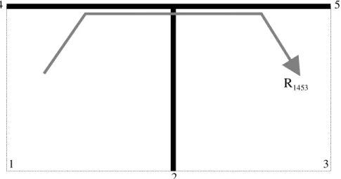
To derive an expression for the first-order flanking paths, consider the simple situation where two rooms are separated by a common wall, as shown in Figure 1. In this situation there will be 12 first-order flanking paths and one direct path (123). To create a first-order prediction model it is sufficient to derive the expressions for an arbitrary first-order flanking path. The path 1453 has been chosen where the number indicates the building component involved in the path. Thus, 1453 begins in the source room (1) which imparts energy into the source
room flanking surface (4) which is connected to the receive room flanking surface (5) by the “tee” junction involving the partition wall. The final element is the receiver room (3). 1 2 3 4 5
R
1453Figure 3.1: Two rooms 1 and 3, separated by wall 2, and the flanking walls 4 and 5.
Using SEA power balance expressions5 one can immediately write the airborne level difference between the source and receiver rooms for an arbitrary path as,
⋅⋅ ⋅⋅ = −1 1 1 .... 1 10log V V D n n n n ij j i i n ij
η
η
η
η
η
η
( 1 )where
η
i refers to the total loss factor (TLF) and ηij to the coupling loss factor(CLF) from subsystem i to subsystem j, V1 is the volume of the source room,
while Vn is the volume of the receiver room.
When computing the level difference between the source and receiver rooms a path is one that:
a.) Begins in the source room and finishes in the receiver room;
b.) The source subsystem appears only once, (i.e., at the start of the path); c.) Other subsystems appear any number of times as long as the CLF between
adjacent subsystems in the path is non-zero, (i.e., it must be acoustically coupled to adjacent subsystems in the path. 1243 is not a path in Figure 3.1 because 4 is not acoustically coupled to 3).
This method works well for low-order transmission paths in comparatively simple structures like that shown in Figure 3.1 were the paths can be written by inspection. First-order paths are 1253, 1423, and 1453. Higher orders in more complex structures generally require the use of a computer algorithm to determine the possible paths and compute the airborne level difference associated with each.
To develop a mathematical expression for first-order flanking paths (i.e., those involving a single source and receive surface and a single junction) it is sufficient to consider an arbitrary first-order path as the resulting expression is generally applicable to other first-order paths by appropriate changes to the subsystem indexes of the CLF and TLF. The path 1453 will be considered. Using equation 1, the sound pressure level difference for the specific transmission path 1453 is = 1 3 53 3 45 5 14 4 1453 10log V V D
η
η
η
η
η
η
( 2 )where V1and V3 are volumes of the source and receiver rooms, respectively. The
first term in the right-hand side of equation 2 can be separated into three terms, as indicated by the braces, each corresponding to a different transmission mechanism. The first term corresponds to coupling from the air volume (1) of the source room to the flanking surface (4) in the same room, while the second term corresponds to coupling across the junction connecting flanking surfaces (4) and (5), and the final term corresponds to coupling from the receiver room flanking surface (5) and the receive room air volume (3).
Thus, SEA provides a general framework for evaluating transmission paths in buildings. However, it is only when the contribution of all possible transmission paths to the receiver room subsystem are summed that the airborne level difference between the source and receiver rooms is approximated. Failure to include important paths, which in addition to first-order paths will include paths of second or higher order, will result in an overestimation of the airborne level difference between source and receiver rooms.
It is common in building acoustics to use the flanking sound reduction index (flanking SRI) to express the sound insulation of a specific transmission path. The flanking SRI is the SRI of the separating wall when the energy transferred through the flanking path would be transmitted through the partition wall. It is obtained by normalizing the airborne level difference for a specific transmission path to the area of the element nominally separating the source and receiver rooms, and the receiver room absorption A. Equation 3 shows the SRI
expression for path 1453, R1453, where rooms 1 and 3 are separated by
element 2, 3 2 1453 1453 10log A S D R = + ( 3 )
The flanking SRI for an arbitrary path of interest would be obtained by using equation 3 with the airborne level difference for the path of interest.
Expressions for the CLF’s and total loss factor (TLF) have already been derived so a derivation will not be given here. Coupling between the air volume of the room (1) and the source room flanking surface (4) is a function of the radiation efficiency of the flanking surface and is given by5,
3 4 s 1 4 4 c 4 2 0 o 14 f V 8 f S c ρ π σ ρ = η ( 4 )
where
σ
is the radiation efficiency,ρ
oco is the characteristic impedance of air,ρ
s is the surface density, f is the frequency, and V is the room volume. A similarexpression exists for coupling from the receive room flanking surface (5) to the receiver room air volume (3)5,
f c s o o 5 5 53 2
πρ
σ
ρ
η
= ( 5 )The coupling loss factor for the joint between the two flanking surfaces (4 and 5), which are assumed to be homogeneous and isotropic, is given by5,
4 4 2 45 45 45 c o ff S L c
π
τ
η
= ( 6 )where L45 is the junction length, and τ45 is the power transmission coefficient for
bending waves through the junction connecting elements 4 and 5. For an arbitrary junction there will be coupling between all three wave types (bending, longitudinal and transverse). However, since bending waves are primarily responsible for radiation the other two types are often ignored, especially when there are few junctions in the path. Ignoring the other wave types and the conversion of energy between them can lead to significant errors for flanking paths with many junctions9,10.
Since it has been assumed that the flanking elements are homogeneous and isotropic the critical frequency can be expressed5 as a function of the modulus of elasticity, E,
(
)
2 1 3 2 2 1 3 − = Eh c fc o sµ
ρ
π
( 7 )where h is the thickness of the element, µ is the Poisson’s ratio and typically
taken to be 0.2 – 0.3 for most structural building materials.
Note that the CLF from the room air volume to the flanking surface is not the same as from the flanking surface to the room air volume. This may appear
somewhat confusing at first however it must be recognised that the constant of proportionality is the ratio of the modal densities5,20, namely
i j ji ij n n =
η
η
( 8 )where n is the modal density. Equation 8 is often referred to as the consistency
relationship. It has important implications as it clearly reveals that the SEA expressions for the flanking SRI (equation 3) consider only transmission involving resonant motion caused by natural modes of vibration. The latter is characterised by the response of a group of eigenmodes with eigenfrequencies in the frequency band of interest. When excited randomly (e.g. by means of a diffuse sound field) all modes will on average respond at resonance, and the amplitude of the resultant vibration will be inversely proportional to the damping. Apart from the damping, the flanking SRI due to resonant motion is also affected by boundary conditions and dimensions, which influence coupling between subsystems as in the specific case of radiation from a plate below the critical frequency12. Although boundary conditions will affect eigenfrequencies of individual modes, they do not determine the overall properties an SEA subsystem as long as a sufficient number of modes are present in the frequency band. Conversely, non-resonant motion is not overly dependent on the damping. This weak dependence on damping is a very important issue when relating the SRI of a flanking path to the SRI of the elements in the path and will be discussed in more detail in Section 5.
For equation 8 and SEA to be valid there must be modes of vibration and that at low frequencies, where there may be few or no modes, the resulting SRI expression(s) are not valid. Fortunately indicators have been developed to help provide guidance in the applicability of SEA in the low frequencies. This will be discussed in more detail in Section 4.
Substituting equations 2, 4, 5, and 6, in equation 3 and combining Sabine's equation for room absorption, A,
A V
RT =0.161 ( 9 )
and the classical relationship11 between TLF and reverberation time,
RT f 2 . 2 = η ( 10 )
gives the flanking sound reduction index as,
= 4 45 45 5 4 3 2 4 5 5 4 4 2 3 3 1453 2 log 10 c o o c S S f L c ff S f R
τ
σ
σ
ρ
η
ρ
η
ρ
π
( 11 )Equation 11 is a general expression for first-order flanking paths and shows that flanking sound reduction can be improved by increasing the damping of the flanking surfaces (elements 4 or 5), reducing their radiation efficiency, or reducing junction transmission (product of the junction length and the junction transmission coefficient).
Perhaps, the most difficult part of evaluating equation 11 is determining appropriate values for the in-situ values for the radiation efficiency, total loss factors and junction transmission coefficient. Reasonable estimates12 for the radiation factor of a rectangular plate of dimension L1 and L2 in an infinite baffle
can be obtained from asymptotic expressions when there are many plate modes,
(
)
(
)
c c c o c c o f f f f f f c f L L L f f L L f f c L L > − = = − = < − + − + − + = − 2 1 2 / 1 2 1 1 2 2 / 1 2 2 1 2 / 1 2 / 1 2 2 1 1 2 15 . 0 5 . 0 1 2 1 1 ln 1 4 ) ( 2σ
π
σ
µ
µ
µ
µ
µ
π
σ
( 12 )where it is assumed that L1 is greater than, or equal to, L2, and
µ
=(
fc/ f)
1/2.Below the critical frequency, plate radiation is enhanced when it is bounded by rigid surfaces that are at right angles to the plate. The radiation may be enhanced (by a further factor of two) if the edges are clamped.
The junction transmission coefficient must be computed for the particular situation as it will be a function of the type of junction (“tee” or “cross”) and whether it has a column or some other structural element at the intersection of the plates. Mathematical models have been created for many types of junctions and many account for the moment of inertia and shear deformation introduced by beams at the joint13,14. Unfortunately, these expressions are sufficiently complex, involving all wave types, that a closed form solution can not be written simply. The same is true for joints for which the plate elements are not connected continuously along the length of the junction but are attached by a series of point connections15,16. Approximate closed form solutions can be written for simple bending transmission corner, tee and cross-junctions which are line-connected and do not have beams. For these, the reader is referred to References 5 and 11.
Since by definition the TLF is the sum of all coupling loss factors5 (which includes transmission to structural elements, and radiation) as well as internal losses (to heat), it too must be calculated
i N i j j ij i int, , 1
η
η
η
=∑
+ ≠ = ( 13 )where j is the index to the subsystem connected to the ith system, ηint,iis the
internal loss factor, and N is the total number of subsystems acoustically coupled
to subsystem i. If the subsystem index i refers to a subsystem that is a room the
CLF, ηij, is evaluated using equation 4 and ηint,i is determined by the amount of
absorption present in the room (losses due to air absorption are assumed negligible). If i is a building element then ηijis evaluated using equations 5 and 6
and ηint,i is typically taken to be 0.015 for concrete and masonry materials. It has
been shown that if the surfaces at the junction have similar thickness and are made of concrete or masonry then the total loss factor for the building element surface may be approximated17 by
015 . 0 1 + = f
η
( 14 )It must be stressed that equation 14 will not be a good approximation for all situations and its use will result in reduced accuracy.
4. Assumptions and Limitations of the SEA Expressions
As with most prediction methods the accuracy of the prediction is only as good as the assumptions made in the underlying theory and how well these are approximated by the system being modelled. SEA is no exception so this section examines four commonly used criteria for establishing the suitability of the method.
Mode Count: The accuracy of SEA predictions is related to the number of modes present in a frequency band. In general, the accuracy increases with increasing mode count. The minimum number of modes required in a subsystem depends on the error that can be tolerated but also on the type of structure being considered. Within the literature there are many values given for the minimum number of modes ranging from 2 to over 30 in a frequency band5,21. It has been suggested for building structures, there should be at least 2 modes5 while other suggest a range of at least 3 to 5 modes18 in each frequency band for which results are to be reported. The mode count is simply the product of the modal density (bracketed term) and bandwidth, f∆ ,
f c Sf f f n f N o c plate ∆ = ∆ = ∆ ) ( ) 2 (
π
( 15 ) f c V f f f n f N o room ∆ = ∆ = ∆ ) ( ) 4 32 (π
( 16 )Since one-third octave bands are often used in building acoustics 3 / 1 f 232 . 0 f =
∆ where f1/3is the one-third octave mid-band frequency. It must be recognised that these expressions are derived from the product of the filter bandwidth and the modal density which is a statistical estimate assuming a uniform distribution of modes. This will not be a very good approximation for low order modes and it may be more accurate to compute the actual modal frequencies where closed form expressions exist19.
Modal Overlap Factor: The modal overlap factor is defined as the ratio of the average modal bandwidth to the average modal frequency spacing. When taking the half power bandwidth for the modal bandwidth, the modal overlap factor is given by, η f f n M = ( ) ( 17 )
It should be noted that another definition of M exists, which is based on a different expression for the modal bandwidth20.
When the modal overlap factor is less than unity some portion of the frequency spectrum may not be controlled by damping. This situation is caused either by a low mode count and/or by low damping. SEA only considers resonant transmission by coupling between groups of modes that represent SEA subsystems. This assumption is not satisfied when there are no modes in a frequency band, or when the modes are widely spaced in terms of modal bandwidth. In the case of two arbitrary subsystems with low modal overlap there is a tendency for SEA to overestimate the coupling between modes of both subsystems and hence the CLF. This can be explained by the fact that the probability that modes of one subsystem will couple to modes of another subsystem becomes small when the resonance peaks are narrow or widely spaced. For most realistic situations in buildings, a low modal overlap will tend to cause an overestimation of the transmission and therefore an underestimation of the flanking SRI. In literature21, the modal overlap factor has been related to uncertainty of SEA predictions. Although a value of M=1 is often suggested, a minimum modal overlap factor depends on the desired accuracy as well as on the type of structure being considered. The uncertainty in the CLF between two plates for bands where there are no modes has been related to the modal overlap factor of the receiving subsystem21. This defines a lower limit of the uncertainty interval of the CLF ηijand is given by,
ij j M 4 Limit Lower η π = ( 18 )
and is valid for Mj<π/4. In monolithic building structures, damping is relatively high so that a unity modal overlap factor can be achieved when only 2 modes are present in a frequency band5.
When the statistical mode count Nplate,j
( )
∆f of the receiving subsystem (obtained from equation 15) is less than unity the upper limit of the uncertainty interval of the CLF ηij is given21 by,( )
f N Limit Upper j , plate ij ∆ η = ( 19 )Note the statistical mode count is a decimal number. Also the uncertainty estimates provided by equations 18 and 19 should not be interpreted to mean that there will be no uncertainty in the CLF estimate when the source plate has no modes but the receiver plate has many modes and a large modal overlap. Weak Coupling: The concept of weak coupling is required to ensure that there are separate modes in both subsystems and that an energy level difference exists between them. Without “weak” coupling the coupled elements are said to be “strongly coupled” and tend to behave as a single subsystem having similar modal energies and in principal no net power will flow. There is no universally accepted point at which two systems cease to be “weakly coupled” and become “strongly coupled.” It has been suggested that strong coupling occurs when the energy transfer to one subsystem is stronger than the energy dissipation in the subsystem, namely when22,
i int, ij >η
η ( 20 )
Although it is generally accepted that SEA should not be used in cases where there is strong coupling, nevertheless there have been both theoretical and experimental studies which show that SEA gives the correct prediction even if strong coupling occurs. This is especially true when the coupled plates have similar wave numbers and have a long junction length23.
Reverberant to Direct Energy: Unless special extensions have been made to SEA theory24 it is assumed that the vibration energy is controlled by the reverberant field (energy that has undergone at least one reflection from a boundary) and that the direct field from all sources is small by comparison. This ensures that the energy density is reasonably uniform over the subsystem so the intensity incident on a boundary occurs at all angles and is a function of the group speed and the mean free path length. The reverberation radius, (the distance from a point source at which the direct field is equal to the reverberant) is often used as a criterion20,
) 1 ( 2
α
η
− = o c plate c ff S R ( 21 ) ) 1 ( 16π
α
α
− = S Rroom ( 22 )where equation 21 is applicable to plates and 22 is applicable to rooms. In both cases S is the surface area, α is the mean power absorption coefficient at the boundary of the subsystem. When the reverberation radius is comparable to the dimensions of the subsystem then the field will no longer be controlled by the reverberant field and SEA will incorrectly estimate the transmission.
5. SEA Expressions using Measured Acoustical Properties of the Elements
Rather than compute the many acoustic quantities of equation 11 such as the radiation efficiency, critical frequency, etc. it may be more convenient to use an expression that has been simplified and uses measured SRI data for the nominally identical building element. The following is a derivation for such an expression.
By reciprocity R1453 is identical to R3541. Thus, the following can be written and
equation 11 modified to,
2 1 54 54 5 5 4 3 2 5 5 2 4 5 3 45 45 4 5 4 3 2 4 5 2 4 4 3 3541 1453 1453 2 2 log 10 2 = + =
τ
σ
σ
ρ
ρ
ρ
η
π
τ
σ
σ
ρ
ρ
ρ
η
π
L f c ff S f L f c ff S f R R R c o o c s s c o o c s s ( 23 )This expression can be factored to reveal the presence of the flanking SRI for elements 4 and 5, R4 and R5, respectively,
2 1 54 54 45 45 2 5 4 4 5 4 2 2 5 2 5 2 2 2 5 5 3 4 2 4 2 2 2 4 4 3 1453 2 2 log 10 =
τ
τ
π
η
η
σ
ρ
ρ
η
π
σ
ρ
ρ
η
π
L L c f f f S f c f f c f R o c c c o o s c o o s ( 24 )where the two terms in the round brackets are the in-situ transmission coefficients for resonant transmission through plate elements 4 and 5, respectively. Since the total loss factor and the radiation efficiency are a function of the mounting conditions and the size of the plate, a distinction must be made between in-situ values and those measured elsewhere, say in a laboratory. We shall add the subscript “L” to those parameters affected. Thus equation 24 can
be rewritten as, 2 1 54 54 45 45 2 5 4 4 5 4 2 2 2 5 2 5 5 5 5 2 4 2 4 4 4 4 1453 1 1 log 10 =
τ
τ
π
η
η
σ
σ
η
η
τ
σ
σ
η
η
τ
c L L f f f S R o c c L L L L L L ( 25 )2 1 2 5 2 5 5 5 2 4 2 4 4 4 2 1 54 54 45 45 2 5 4 4 5 4 2 2 , 5 , 4 1453 10log 10log 2 + + + =
σ
σ
η
η
σ
σ
η
η
τ
τ
π
η
η
L L L L o c c res res L L c f f f S R R R ( 26 )The subscript “res” has been added to explicitly note that it is the resonant
component of the measured sound reduction index that must be used. As discussed in Appendix A, SRI measured in accordance with standardised transmission loss test methods employing a reverberant source room (e.g., ISO 140, ASTM E90, or ISO 15186) is the resultant of two transmission mechanisms, resonant and non-resonant. Appendix A shows that for monolithic elements the resonant sound reduction can be approximated by the measured sound reduction index only for frequencies greater than the critical frequency. This is the frequency range where the radiation efficiency should be reasonably independent of the plate geometry and mounting configuration as demonstrated by equation 12.
Equation 26 really is not any simpler than equation 11 because of the need to retain terms relating to the in-situ radiation efficiency and the total loss factors in addition to new terms describing the conditions for the measured data.
Comparison of the EN12354 and SEA Expressions
It will be shown that using the EN12354 expression for the airborne sound reduction index of a flanking path is in fact the same as equation 26 when a number of simplifying assumptions are added. The procedure begins by using equation E1 of Annex E of EN12354 to obtain an expression relating the junction transmission coefficient in terms of the junction vibration reduction index, Kij,
+ = 5 4 2 45 2 1 54 45 log 5 1 log 10 c c ref f f f K
τ
τ
( 27 )where fref is the “reference frequency” and takes the value of 1000 Hz.
Substituting equation 27 into equation 26 gives,
2 1 2 5 2 5 5 5 2 4 2 4 4 4 2 1 54 45 2 4 5 4 2 2 45 , 5 , 4 1453 10log 10log 2 + + + + =
σ
σ
η
η
σ
σ
η
η
π
η
η
L L L L o ref res res L L c f f S K R R R ( 28 )EN12354 does not explicitly use the total loss factors in its expression, but rather uses the concept of an “equivalent absorption length” -- the length of a fictional totally absorbing edge of an element if its critical frequency is assumed to be 1000 Hz giving the same loss as the element in a given situation. Using equation 22 of EN12354 we obtain an expression for the total loss factor of the flanking elements 4 and 5 in terms of the “equivalent absorption length”, a,
ref situ f f S c a 4 2 0 , 4 4
π
η
= , ref situ f f S c a 5 2 0 , 5 5π
η
= ( 29 )Equation 29 allows equation 28 to be simplified to,
2 1 2 5 2 5 5 5 2 4 2 4 4 4 5 , 5 4 , 4 45 2 45 , 5 , 4
1453 10log 10log 10log
2 + + + + + = σ σ η η σ σ η η L L L L situ situ res res S a S a L S K R R R ( 30 )
Equation 30 is identical to equation 25 of EN12354 Part 1 when:
a.) The EN12354 expression uses the resonant sound reduction index for the flanking elements;
b.) The EN12354 expression assumes that the radiation factors and total loss factors are the same for both the input data and in-situ conditions.
The general procedure used in this paper and SEA framework allows for the simple description of first-order (equations 11 and 30) and second-order flanking transmission (equations B2 and B5). The sound reduction index of a first-order (or a second-order) flanking path is a function of the surface density, total loss factor, and radiation efficiency of both flanking elements, the junction transmission coefficient and length, as well as the critical frequency when the flanking elements can be considered homogenous and isotropic. There are no terms involving the source and receive room volumes, as expected.
The derivation of the SEA formulation clearly indicates that the transmission mechanism is by resonant modes of vibration and that if the expressions are rewritten in terms of the SRI of the flanking elements then it is only the resonant component of the SRI that should be included. This is fully consistent with the suggestion of EN12354 that the resonant component be used over the whole frequency range of interest.
6. Discussion of the Expressions
This section discusses the resulting first-order expressions and identifies the more significant sources of random and bias error. Random errors are generally associated with one or more of the building elements not adequately satisfying the requirements for a subsystem. Whereas bias errors are caused by arbitrarily limiting calculations to first-order paths as well as using input data (e.g., element SRI and junction attenuation obtained from measurement situations) that are inconsistent with assumptions made in formulating the expressions. A method for estimating the potential error associated with using measured data for the flanking element SRI is discussed in detail in Appendix A and Appendix B extends the derivation of Section 5 to provide an expression suitable for second-order flanking paths involving two junctions.
Sources of Bias Error
The three most notable sources of bias error associated with the first-order expressions are:
a.) Assuming that the apparent sound reduction index between two rooms separated by a common wall or floor can be predicted sufficiently accurately from the direct transmission path and the sum of the twelve first-order flanking paths. This causes the total power transmitted to be underestimated and the apparent SRI to be overestimated.
b.) Assuming, that when using measured data for the SRI of the flanking elements, the non-resonant component is negligible with respect to the resonant component over the frequency range of interest. This causes the power transmitted by the (computed) flanking paths to be overestimated and the apparent SRI to be underestimated.
c.) Assuming, that when using measured data for the junction attenuation, the measurement conditions are consistent with those implicit in the expressions. In-situ measurements using the simple method for measuring junction attenuation implied by EN12354 and often used in SEA5 underestimates junction attenuation and underestimates the flanking SRI for paths involving that junction.
The magnitude and relative importance of the three bias errors will change depending on the construction details of the building being modelled. They are now discussed.
The first source of bias error is inherent to the formulation which is the assumption that the apparent sound reduction index between two rooms separated by a common wall or floor can be predicted sufficiently accurately from the direct transmission path and the sum of the twelve first-order flanking paths. The magnitude of the bias error is a complex function of the sound insulation of the separating element, the geometry of the rooms and the damping of the elements. It has been shown from theoretical calculations9 using SEA to be as large as 5 dB. It is possible to reduce this bias and increase the accuracy of EN12354 predictions by including the contribution of from both first and second-order flanking paths. A second-second-order path involving two junctions may be evaluated using the expression provided in Appendix B.
The second source of bias error may partially explain why the 2 dB bias reported25 for EN12354 predictions of heavy monolithic assemblies is lower than the 5 dB suggested by SEA theory. This is because assuming that the non-resonant component present in measured SRI data is negligible with respect to the resonant component will tend to underestimate the SRI for paths involving these elements as shown in Appendix A. This bias tends to offset the bias error associated with limiting the prediction to first-order paths. This should not be taken as an argument for retaining the non-resonant component as the two opposing biases are not physically related. Rather, the bias should be reduced by using input data that are consistent with the assumptions of the expression
formulation and by including higher orders in the prediction. (Appendix B provides the derivation of an expression for higher orders).
For homogeneous monolithic elements the resonant SRI can be obtained by direct calculation or by applying a correction to measured data for frequencies below the critical frequency. Appendix A shows the magnitude of the bias error increases as the critical frequency moves further into the building acoustics range. If the input data require correction for the non-resonant component then it is necessary to consider the effects of differences in damping and element radiation efficiency. Since this correction requires computing estimates of the resonant transmission and the total transmission (sum of the resonant and non-resonant components) and taking the logarithm of the ratio, it would be considerably simpler and perhaps more accurate to use a computed estimate of the resonant component. Thus, it would seem that using measured input data would only be of advantage when the critical frequency of the flanking element is sufficiently low (i.e., below the building acoustics range) so that the measured data are dominated by resonant transmission and it is not necessary to apply a correction.
Unfortunately, to properly investigate the bias it is necessary to have access to all material properties, dimensions, etc., which are often not presented in the literature. It is suggested as future work, for those that have the data, to investigate if removing the non-resonant component of the input SRI improves the accuracy of the flanking SRI for heavy monolithic constructions. The need to remove the non-resonant component has been identified for lightweight assemblies26.
The other potential source of bias error associated with the input data comes from estimates of the junction attenuation (Kijfor EN12354, and
τ
ij for SEA) which can be obtained either by measurement or by prediction. In general, junction attenuation is measured indirectly using measures of velocity level difference and assumptions about possible transmission paths between the two elements coupled by the junction5. In a real building, and likely most laboratory situations, the measured velocity level difference between two coupled building elements will be due to power transmission not only directly across the common junction but also by the many other paths. Thus, assuming that these other paths are negligible and that all the power was transmitted through the common junction (which is implied in Section 4.2.2 of EN12354) is clearly an approximation of a much more complex system. The result is an underestimation of the attenuation of the junction connecting the two building elements. The magnitude of the underestimation depends on the measurement situation. The largest errors will occur when the actual transmission between the coupled elements is weak and transmission via the other paths is strong. This is discussed in more detail in Refs. 5 and 9. Calculated estimates of junction attenuation should not suffer from the inclusion of additional and unwanted paths as measured data invariably do. Thus, it is quite possible that there aresituations where it is more accurate to predict junction attenuation than to use estimates obtained from a simple velocity level difference measurement across the junction.
Random and Other Sources of Error
Beyond the obvious limitation imposed by the low-order prediction, the accuracy will be determined not only by the accuracy and validity of the input data but also by how well the assumptions of the underlying SEA theory are satisfied for the structure under consideration. SEA predicts the average response of an ensemble of similar systems with randomly varying physical properties20. This implies that the response of any individual member of the ensemble will differ from the ensemble averaged response. Since the corresponding error generally decreases with increasing frequency, SEA is often referred to as a mid- and high frequency prediction method. At low frequencies, the concept of ensemble averaged response is still valid, however the difference between the average response and the response of an individual system may be unacceptably high. The user should check the appropriateness of SEA by evaluating the mode count or examining the lowest modal frequencies. The effect of a low mode count can be partially offset by the damping. The resulting criterion is the modal overlap (Section 4) and should be evaluated in the low frequencies to ensure that the system is damping controlled.
High damping increases the modal overlap factor and low frequency accuracy but excessive damping can lead to a situation, especially in the high frequencies, where the reverberation radius is comparable to the dimensions of the subsystem. The resulting field may not be dominated by the reverberant field but instead is controlled by the direct field from the source(s) which violates a fundamental requirement of SEA.
7. Conclusions
SEA provides a simple and effective framework to create expressions to describe flanking transmission in buildings constructed from homogeneous, isotropic monolithic elements that are moderately damped. Criteria are given to help assess the suitability of the expressions to a particular situation as accuracy will be compromised when, in one or more subsystems, there is a.) low mode count, b.) low modal overlap, c.) strong coupling, or d.) excessive damping and the vibration response is no longer controlled by the reverberant field.
The EN12354 expressions were not derived explicitly using a framework such as SEA and as a result the EN12354 expressions do not have a set of criteria to help assess the applicability of the method. The ability to derive the EN12354 expressions from SEA would suggest that the SEA criteria should be considered when applying the standardised EN12354 prediction model.
Both the SEA and EN12354 expressions are deceptively simple and without full appreciation of the underlying assumptions it is possible to apply them to
Appendix A: Obtaining estimates of the resonant sound reduction index using data obtained from ISO 140.
If the coupling loss factor(s) from a surface to a room, and visa versa, are to be expressed in terms of measured sound reduction data then it is necessary to ensure that the SRI is only for resonant transmission. Unfortunately, standardised methods for estimating the sound reduction index (such as ISO 140 and ASTM E90) provide an estimate of the resultant sound insulation due to both resonant and non-resonant transmission mechanisms, namely,
+ = −resonant non resonant R
τ
τ
1 log 10 ( A1 )If the surface is monolithic and the critical frequency is well below the frequency range of interest (typically 100-5000 Hz) then it should not be necessary to correct for the non-resonant component as it will be negligible with respect to the resonant component and measured data can safely be used.
However, if the critical frequency is in the frequency range of interest then it is necessary to correct for the non-resonant component. An experimental technique26 has been reported but required very detailed measurements of ratio between surface velocity and the incident sound intensity when the surface was exposed to airborne sound excitation and the ratio of surface velocity to radiated sound intensity when the surface was excited mechanically at an edge. Clearly, this is not practical, except for laboratory situations. Consequently, an alternate method based on theoretical expressions is given and compared to measured results.
It is highly desirable to have a simple expression to remove the non-resonant component which is included in standardised measures of sound reduction index measured using the standard two-room technique (of ISO 140 or ASTM E90), namely, c f f C ISO resonant R R R = 140 + , < ( A2 )
where the subscript f<fc indicates that it is only necessary to apply the
non-resonant correction expression, Rc, for frequencies below the critical frequency.
By inspection of equation A1, RC,f<fc must take the form,
+ = − < resonant resonant non resonant f f C c R
τ
τ
τ
log 10 , ( A3 )We shall restrict the discussion to single leaf building elements as this is sufficient to illustrate the importance of removing the non-resonant component, although it is equally important for double leaf assemblies but unfortunately a closed form expression does not exist.
For airborne transmission through a monolithic element below the critical frequency, the resonant transmission coefficient5 is given by,
= < < tot f f resonant c s o f f resonant c c f f f c
η
σ
π
ρ
π
ρ
τ
2 , 2 0 , 2 ( A4 )where the radiation efficiency is given by equation 12. The non-resonant transmission coefficient is given by27,
(
)
( )
+ − + − = − < −ξ
µ
π
µ
ρ
π
ρ
τ
1 2 2 1 2 4 2 , 0.160 2 ln 1 1 L L U c L L f f c o s o o f f resonant non c ( A5 ) where,( )
(
)
( )
( )
( )
dt t t x x x x x x U x∫
− − + − + + = 2 ln 2 2 1arctan ln 2 2 1 1 ln 1 2 1π
π
π
( A6 ) and( )
(
(
µ
)(
µ
) (
µ
) (
µ
)(
µ
) (
µ
)
µ
µ
( )
µ
)
µ
µ
ξ
2 1 1 ln 1 2 1 1 ln 1 4 8 ln 4 1 2 2 2 2 2 2 2 2 2 6 6 − + − + + − + − − = ( A7 )and where L1 and L2 are the length and width of the surface,
µ
= fc/ f and theother quantities have been previously defined in this paper.
Substituting equations A4 and A5 into equation A3 gives an expression for the non-resonant correction that must be added to the measured SRI for a monolithic element to obtain an estimate of the resonant sound reduction index,
(
)
( )
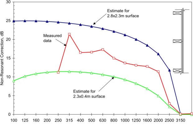
+ − + − + = − < tot resonant c o tot resonant c f f C f f L L U c L L f f f Log R c η σ π µ ξ π µ η σ π 2 1 2 2 1 2 4 2 , 2 160 . 0 2 ln 1 1 2 10 ( A8 )An estimate of the magnitude of the non-resonant correction using equation A8 is shown in Figure A1 for a 2.8 x 2.3 m building element consisting of double layer of 13 mm gypsum board mounted on 38 x 89 mm wood studs spaced 400 mm on centre. The critical frequency was estimated to be 3150 Hz from measured data and the surface density was taken to be 21.0 kg/m2. Also given are the measured data from reference 26 for the same structure.
The figure indicates that the effect will be a function of the size and dimension of the building element. The smaller building element having a higher aspect ratio exhibits a smaller correction because these surfaces are more efficient radiators than large square surfaces, especially at low frequencies. This accounts for increasing difference between the two predictions as the frequency is decreased.
0 5 10 15 20 25 30 100 125 160 200 250 315 400 500 630 800 1000 1250 1600 2000 2500 3150 Frequency, Hz Non-Resonant Cor re ct ion, dB Estimate for 2.8x2.3m surface Estimate for 2.3x0.4m surface Measured data
Figure A1. Estimates of the correction that must be added to sound reduction index data (measured using ISO 140, ISO 15186 or ASTM E90 test methods) to obtain an estimate of the resonant sound reduction index for a single leaf wall consisting of a double layer of 12.7mm gypsum board on 38x89mm wood studs spaced 400mm on centre. The predictions were obtained from equation A8 measured data were taken from reference 26.
Regardless of the effective dimension, the measured data indicate that the correction is likely to be greater than 15 dB for frequencies one octave, or more below the critical frequency (3150 Hz). If the critical frequency falls near the upper end of the building acoustics frequency range, as it does for lightweight walls, then using sound reduction index data obtained from of standardised
measurement methods (e.g., ISO140) without accounting for the non-resonant component, will result in a very serious (15 dB) underestimation of the resonant sound reduction and hence the flanking sound reduction index.
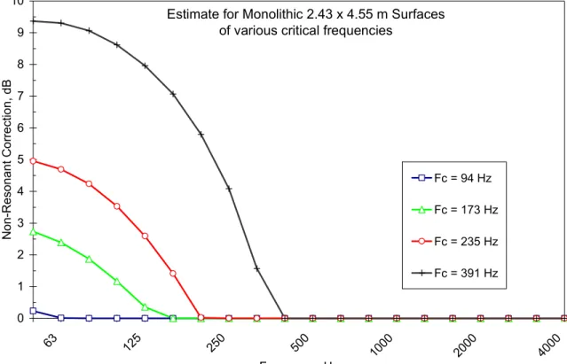
The magnitude of the correction increases very rapidly for frequencies just below the critical frequency so there may also be a significant effect for heavy monolithic elements such as cast-in-place concrete. This suggests that it might be necessary to account for the non-resonant component even for heavy monolithic elements. Figure A2, which shows estimates of the non-resonant correction for various concrete and masonry materials, indicates that if the bias error is to be kept below 1 dB throughout the building acoustics range, then it will be necessary to apply a correction to the SRI data when the critical frequency occurs above about 200 Hz. This threshold will move lower as the ratio of area to perimeter length increases.
Failure to correct for the non-resonant component may be used to introduce a deliberate underestimation in the flanking sound reduction, however this underestimation can be significant and may range from 0 to in excess of 10 dB depending on the critical frequency and the dimensions of the building element. Thus, failing to correct for the non-resonant component is not a reliable method of introducing a margin of safety.
0 1 2 3 4 5 6 7 8 9 10 63 125 250 500 100 0 2000 400 0 Frequency, Hz N on-R es onant C or rec ti on, dB Fc = 94 Hz Fc = 173 Hz Fc = 235 Hz Fc = 391 Hz
Estimate for Monolithic 2.43 x 4.55 m Surfaces of various critical frequencies
FIGURE A2. Estimates of the correction that must be added to sound reduction index data (measured using ISO 140, ISO 15186, or ASTM E90 test methods) for various concrete and masonry monolithic elements to obtain an estimate of the
resonant sound reduction index. The predictions were obtained from equation A8. The materials are identified by the critical frequency, fc=94: 200 mm thick concrete, fc=173 Hz: 100 mm concrete and 30 mm finish, fc=235 Hz: 100 mm calcium silica blocks, fc=391 Hz 70 mm gypsum blocks.
Figures A1 and A2, demonstrate that equation A8 can be used to assess if there are likely to be significant errors associated with using measured SRI data for the flanking elements. It is likely that more accurate estimates of the in-situ resonant sound reduction index can be obtained by direct calculation using equation A4 than by applying a non-resonant correction to measured data (equation A8). This is because the process to extract the resonant component from measured SRI data (using equation A8) and adjusting the resulting values to in situ conditions (last term of equation 30) requires knowledge of the specimen dimension and TLF, whereas direct calculation requires the surface density, in addition to the specimen dimension and TLF. It is highly likely that the uncertainty associated with estimates of the surface density will be less than that associated with computing the non-resonant component of the SRI used in equation A8.
Appendix B: Expressions for higher order flanking paths
Recently, situations have been presented28, similar to that shown in Figure B1 for path 14653, where a small element (shown as 6) couples a larger element (5) to the junction involving the partition wall. In this case there are two junctions (4-6 and 6-5) in the path each causing vibration attenuation. It was suggested that first-order prediction models based on a single junction and a single flanking surface in each room (as shown in Figure B1) could be simply extended by summing junction terms.
1 2 3 4 R1453 5 R14653 5 3 1 4 6 2
A
B
FIGURE B1. Two rooms 1 and 3 separated by wall 2. In Figure B1A the flanking walls 4 and 5 do not have a coupling element, while in Figure B1B they are coupled by element 6.
The main purpose of this Appendix is not to derive a general expression for flanking paths involving two junctions although this is a required step to show that it is not possible to simply sum the junction transmission coefficients (either expressed as a coefficient of transmitted to incident power,
τ
ijused in the main body, or the Kij of EN12354). In general, this summation will lead to seriouserrors.
We now begin to derive an expression for second-order flanking paths which cross two junctions. Inspection of Figure B1B indicates that there are seven such paths (14263, 12653, 14623, 12423,12463, 12623, and 14653). It is sufficient to choose any one of these paths and compare the resulting expression to that obtained when the Kij’s are summed so assess the validity of summing Kij’s to represent multiple junctions. We have arbitrarily chosen path 14653.
Using equations 1 and 3 of the main body, the sound reduction index for the path 14653 is given by,
+ = 3 1 2 3 53 3 65 5 46 6 14 4 14653 10log 10log A V S V R situ situ situ situ
η
η
η
η
η
η
η
η
( B1 )By inspection this expression differs only from the expression obtained for first-order paths in that equation B1 has two junction terms instead of one. The terms representing coupling to and from the rooms remain unchanged. Thus substituting equations 4, 5, 6, 9, and 10 into equation B1 and using reciprocity gives, 2 1 2 2 56 56 65 65 2 5 6 4 5 6 64 64 46 46 2 6 4 4 6 4 5 2 5 2 2 2 5 5 3 4 2 4 2 2 2 4 4 3 14653 2 2 log 10 = S L L c f f f L L c f f f f c f f c f R o c c o c c c o o s c o o s τ τ π η η τ τ π η η σ ρ ρ η π σ ρ ρ η π ( B2 )
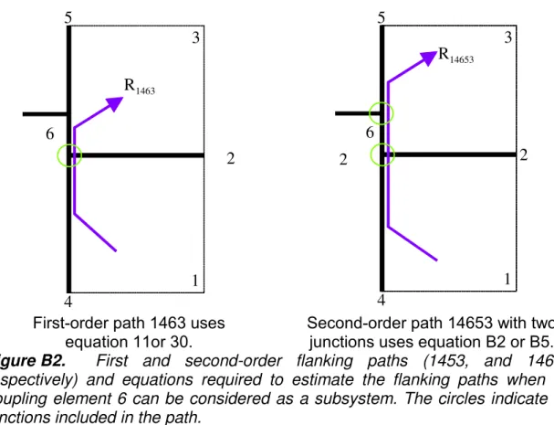
This is a general expression applicable to the situation where the path from the source to receiver subsystems involves four coupling loss factors, two of which involve junctions coupled to element 6 and element 6 satisfies all the conditions of a subsystem. This expression differs from equation 24 only in the presence of an additional coupling term. It is interesting to note that although there is an additional flanking element, 6, in the flanking path described by equation B2, there are no radiation or acceptance terms involving 6. This means that in the formulation, element 6 is a “coupling element” which contributes only to structure borne transmission and not to radiation. In practice this condition will likely never happen if element 6 satisfies the conditions of a subsystem. Thus equation B2 only provides an estimate for path 14653 and does not include a contribution from path 1463. The two paths as shown in Figure B2 must be computed separately. Path 1463 having only a single junction should be evaluated using equation 11 or 30, and path 14653 having two junctions should be evaluated using equation B2.
R1463 5 3 1 4 6 2 R14653 5 3 1 4 6 2 2
First-order path 1463 uses equation 11or 30.
Second-order path 14653 with two junctions uses equation B2 or B5.
Figure B2. First and second-order flanking paths (1453, and 14653, respectively) and equations required to estimate the flanking paths when the coupling element 6 can be considered as a subsystem. The circles indicate the junctions included in the path.
It is possible that the coupling element 6 is a narrow strip and does not support modes. In this case it should not be explicitly considered as an element in the flanking path but rather it should be included as part of the junction. In the example shown in Figure B1 the two junctions would become one and might be modelled as a variant of an “H” junction where element 6 is the coupling member and elements 4 and 5 have been rotated through 90 degrees counter clockwise. The basis for modelling such a joint, assuming a line connection, has already been given29.
Using the same procedure as in the main body of this paper, equation B2 can be expressed in terms of the resonant sound reduction of elements 4 and 5,
2 1 2 5 2 5 5 5 2 4 2 4 4 4 2 1 56 56 65 65 2 5 6 4 5 6 6 2 2 1 64 64 46 46 2 6 4 4 6 4 6 2 , 5 , 4 14653 log 10 log 10 log 10 2 + + + + = σ σ ηη σ σ ηη τ τ π η η τ τ π η η L L L L o c c o c c res res L L c f f f S S L L c f f f S S R R R B 3 )
The first term relates to the acceptance and radiation of energy by elements 4 and 5, while the third and fourth terms relate to the coupling of 4 to 6 and 6 to 5. The final term is required to adapt the measured (laboratory) data to in-situ conditions.
An equivalent expression using the terminology of EN12354 can be obtained by using equation 27 to relate the junction transmission coefficients to the vibration reduction index, Kij. The resulting expression is
2 1 2 5 2 5 5 5 2 4 2 4 4 4 2 1 65 56 2 4 6 5 6 2 2 1 64 46 2 4 6 4 6 2 65 46 , 5 , 4 14653 log 10 log 10 log 10 2 + + + + + + = σ σ η η σ σ η η π η η π η η L L L L o ref o ref res res L L c f f S S L L c f f S S K K R R R ( B4 )
and rearranging the terms
2 1 2 5 2 5 5 5 2 4 2 4 4 4 2 1 65 56 2 4 6 6 2 6 2 1 64 46 2 4 5 4 2 2 65 46 , 5 , 4 14653 log 10 log 10 log 10 2 + + + + + + =
σ
σ
η
η
σ
σ
η
η
π
η
η
π
η
η
L L L L o ref o ref res res L L c f f S L L c f f S K K R R R ( B5 )Note: Equations B2, and B5 are only applicable to flanking paths were there are four coupling loss factors two of which involve junctions.
Comparing equations 30 and B5 indicates that the second junction has added another Kij and a second term,
2 1 2 65 2 4 2 6 2 6 log 10 L c f f S o ref
π
η
( B6 )Thus, if all the junctions have the same length as would typically be the case for walls or floors in buildings, the error in assuming that the Kij’s can simply be
summed is 2 1 2 2 4 2 6 2 6 log 10 = L c f f S Error o ref
π
η
( B7 )where L is the junction length.
While the basic formulation lends itself to extension to multiple junctions it should be realised that extending to higher orders will tend to compound errors
introduced by poor assumptions used in the formulation. Perhaps the most important assumption relates to the coupling element and how to determine if it is sufficiently large to warrant being treated as a separate subsystem. If it is too small then it must be modelled as a component in the junction. The subsystem criteria of Section 4 should provide some guidance.
The number of subsystems and path order necessary to achieve an arbitrary level of accuracy in the predicted airborne level difference between source and receiver rooms is generally not known. So evaluating the airborne level difference using closed form expressions (like equations 30 and B5) becomes an iterative process where the model complexity (path order and number of subsystems) is increased until the difference between consecutive predictions is less than a desired value. Even for the simple case of two rectangular rooms sharing a common wall like that shown in Figure B1A, evaluation beyond the first order (3 CLF’s) will likely require a computer algorithm to determine the possible paths and evaluate the airborne level difference of each. Using the definition given in Section 3, there are at least 86 second-order paths (i.e., having four CLF’s) between room the source and receiver rooms.