Diffusion of diluents in glassy polymers

'IC

Depaftment of Chemical Engineering May 17,1994 /11 I

- . - - - A 0 '%

by

PAUL FRANKLIN NEALEY Bachelor of Science, Chemical Engineering

Rice University, Houston, Texas, 1985

Submitted to the Department of Chemical Engineering in partial fulfillment of the requirements for the degree of

DOCTOR OF PHILOSOPHY in Chemical Engineering

at the

MASSACHUSETTS INSTITUTE OF TECHNOLOGY May, 1994

Massachusetts Institute of Technology, 1994 All rights reserved

Signature of Authoj.

Certified bv 1

Robert E. Cohen, Professor of Chemical Engineering Thesis Advisor

and by

Ali S. Argon, ProjWssor of Mechanical Engineering Thesis Advisor

Accepted by

Robert E. Cohen Chainnan, Committee for Graduate Students

I

Sdencg

Diffusion of Diluents in Glassy Polymers

by

Paul Franklin Nealey

Submitted to the Department of Chemical Engineering on May 17, 1994, in partial fulfillment of the requirements for the degree of

Doctor of Philosophy in Chemical Engineering.

Abstract

A central eature of a recently reported toughening mechanism observed in blends of a few volume percent low molecular weight polybutadiene(PB) in polystyrene (PS) is the localized plasticization of PS by PB in the immediate vicinity of crazes. The sorption of PB into the PS craze matter is driven by the significant concentrations of positive man normal stress, y, at the craze tip and along the craze borders, and throughout the fibrils. 'Me required diffusion coefficient for PB in PS in these regions in craze growth

experiments at 25 T is approximately 1-12 cm2/s.

The thermally-induced diffusion of low molecular weight PB in PS was measured with Forward Recoil Spectroscopy (FRES). Diffusion coefficients were deten-nined for 3000 g/mol perdeuterated PB penetrating into a 350,000 g/mol PS matrix in the temperature range of 97 to 115 'C. The diffusion coefficients vary from -15 to 1-12 cm2/s. The

apparent activation energy, AE, is 99 kcal/mol. The values of D and AE are in good agreement with those found for the diffusion of photoreactive dye molecules in PS in the same temperature range. This implies that the PB molecule acts as a probe of PS matrix properties. The thermally-induced tracer diffusion of PB in PS did not proceed at a rate

equivalent to the estimated rate required by the toughening mechanism until the temperature reached 1 15 'C, a temperature well above the T of PS.

The effect of stress on the diffusion of in PS was investigated by applying gas pressure. Hydrostatic pressure (negative mean normal stress) decreased D from

1.2 x 1-13 to 37 x 1-14 cm2/s as the pressure increased from to 11.3 MPa at 107 'C. On the other hand, D is expected to increase if the PS is subjected to a positive mean normal stress. However, even the largest value of ; in the vicinity of crazes can not fully account for the rapid diffusion of PB in PS in the toughening mechanism at 25 'C.

Diffusion in a model plasticizer/glassy polymer system consisting of resorcinol bis(diphenyl phosphate) (RDP) and a polyetherimide (UltemPll) was investigated to

determine if a non-Fickian diffusion mechanism could account for the flux of PB into PS in the fringe layers of crazes. Volume fraction versus depth profiles of RDP in UltemTm were measured with Rutherford Backscattering Spectroscopy (RBS) as a function of time, temperature, and externally applied stress when RDP was present in a imited supply. In the temperature range of 120 to 180 'C, diffusion front velocities varied from 10-4 to 10-1 nm/s. These experiments are comparable to the PB/PS system on the basis of the temperature difference T -T

_{' to expen}

PB in PS in the diffusion process of the toughening mechanism. Externally applied biaxial stresses in the plane normal to the direction of penetration had no effect on the diffusion.

The diffusion measurements in the PB/PS system and the RDP/UltemTm system reveal that the physical properties of PS during the deformation process are dramatically different than the unstressed polymer or the stressed polymer pior to plastic deformation.

Acknowledgments

This research was supported primarily by NSF/MRL, through the Center for Materials Science and Engineering at M.I.T. under grant No. DMR-90-22933. Other sources of funding included the David H. Koch School of Chemical Engineering Practice at MIT, and a fellowship from Bayer AG.

I consider myself extremely fortunate to have had the opportunity to work with Professors R. E. Cohen and A. S. Argon. Their enthusiasm, interest, and insight created a supportive and intellectually challenging environment in which to learn and to conduct research.

Other people to whom my thanks are due include members of my thesis committee, W. M. Deen, and E. W. Merrill; Professor Kramer and his research group at Cornell University; and Roger Kambour of General Electric Co.

RBS and FRES experiments would have been impossible without the collaboration of John Chervinsky at the Cambridge Accelerator for Materials Science at Harvard

University. Important sample preparation procedures were developed by Alexis Black when she worked as a UROP in our laboratory.

Finally, I will always value the experience of being part of the Cohen group. The frienships that I made in Boston contributed to both my education and my quality of life, and will surely be the most enduring aspect of my time at MIT.

Table of Contents

Abstract ...

3

1. A New Toughening Mechanism for Glassy Polymers ... 13

1.2 The Diffusion Process ... 19

1.3 Research Objectives ... 25

1.4 References for Chapter 1 ... 26

Chapter 2: Ion Beam Analysis ... 29

2.1 Introduction ... 29

2.2 General Concepts ... 30

2.3 Rutherford Backscattering Spectroscopy ... 34

2.4 Forward Recoil Spectroscopy ... 46

2.5 References for Chapter 2 ... 53

Chapter 3 Solubility and Diffusion of PB in PS at Elevated Temperatures ... 56

3.1 Abstract ... 56 3.2 Introduction ... 56 3.3 Experimental Section ... 58 3.4 Results ... 61 3.5 Discussion ... 67 3.6 Summary ... 79

3.7 References for Chapter 3 ... 80 Chapter 4 Ile Effect of Gas Pressure on the Solubility and Diffusion of PB in PS 82

4.1 Abstract ... 82

4.2 Introduction ... 82

4.3 Experimental Section ... 83

4.4 Results and Discussion ... 85

4.5 Summary ... 101

4.6 References for Chapter 4 ... 102

Chapter 5: Limited Supply Non-Fickian Diffusion in Glassy Polymers ... 104

5.1 Abstract ... 104 5.2 Introduction ... 105 5.3 Experimental Section ... 108 5.4 Results ... 112 5.5 Discussion ... 126 5.6 Summary ... 136

5.7 References for Chapter 5 ... 137

Chapter 6: Summary ... 140

List of Figures

Figure 1 I Schematic of a typical stress-strain plot for PS hornopolymer and 1 5

a toughened blend of a few volume percent PB in PS.

Figure 12 Craze propagating in a blend of a few volume percent low 16 molecular weight PB and PS in which the PB is phase separated into small

pools.

Figure 13 Schematic of non-Fickian diffusion profiles at integral times for 20 a constant activity reservoir in contact with a glassy polymer.

Figure 14 Schematic of non-Fickian diffusion profile where the curve 21 marked is the actual concentration profile, oe the local equilibrium

concentration profile, and P the osmotic pressure.

Figure 1.5 Craze fibrils spaced a distance I apart with active zone of 24 thickness h.

Figure 21 Energy loss through a sample of thickness Ax. 32

Figure 22 Configuration of RBS experiment, 0=176'. 35

Figure 23 Schematic of elastic collision in RBS. 35

Figure 24 Schematic of energy losses for a collision at depth Ax in the 37 sample.

Figure 25 Typical RBS data for a sample in which RDP has diffused into 43

UltemTm.

Figure 26 Sensitivity of RUMP fit to RBS data with variation of the 44 'simulated'penetration depth.

Figure 28 Configuration of the FRES experiment. 46

Figure 29 Elastic Recoil Collision in FRES. 47

Figure 2 1 0 Schematic of recoil event in FRES. 48

Figure 211 FRES data from a homogeneous blend of 0.277/0.723 51

dPS/hPS which is 210 nrn thick.

Figure 31 Configuration of FRES experiment. 60

Figure 32 Schematic of a typical sample in the solubility experiments. 63

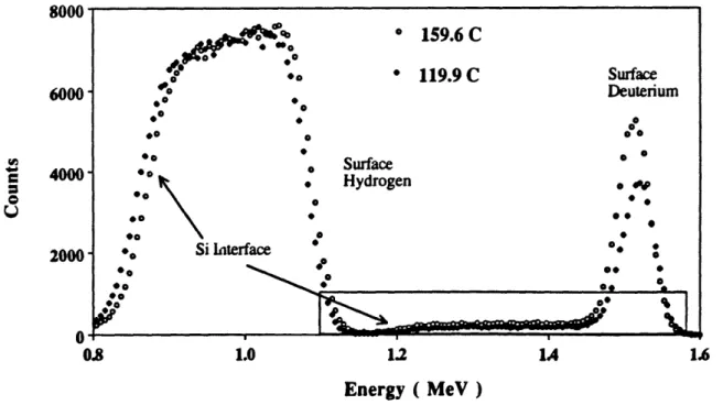
Figure 33 Overview of FRES data for samples held for I hour at 159.6 and 63 119.9 "C.

Figure 34 Expanded view of the deuterium profiles for samples held for 64 hour at 159.6 and 119.9 'C.

Figure 35 Schematic of a typical sample in the diffusion experiments. 65

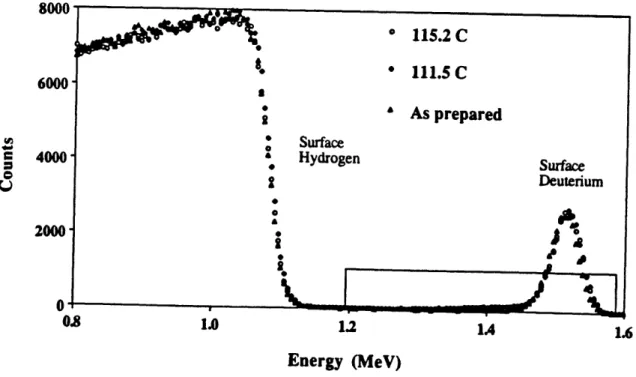
Figure 36 Overview of FRES data for samples held for min at 115.2 and 65 1 1 1.5 'C and an unheated sample.

Figure 37 Expanded view of the deuterium profiles for samples held for 66 min at 1 5.2 and 1 1 1. 5 'C and an unheated smple.

Figure 38 Overview of FRES data and simulation for a sample held for 68 hour at 139.9 'C.

Figure 39 Expanded view of the deuterium profile and smulation for a 68 sample held for hour at 139.9 'C plotted in terms of volume fraction

versus depth.

Figure 310 Plot of temperature versus the solubility of dPB in PS. denotes 71

solubilities determined from FRES data. The solid line is the best fit of a binodal curve to the data with A= 071 - 0.00020(T T). The dashed line is the binodal curve calculated for A = .05 - 0.0022(T 'Q which is based on the results of Roe and Zin.

Figure 3 1 1 Expanded view of the deuterium profile and simulation in terms of volume fraction versus depth for a sample held 15 min at 107.4 'C. The simulation employs a value of C. which was determined from the binodal curve fit to the experimental solubility data.

Figure 312 Expanded view of the deuterium profile and simulation in terms of volume fraction versus depth for a sample held 15 min at 107.4 'C. The simulation employs the best two-parameter fit for values of C. and D.

Figure 313 Semilog plot of D versus 1000/T. The solid line represents the best fit of an Arrhenius equation to the data with AEact = 99 kcal/mole.

Figure 41 Schematic of a typical sample in the solubility experiments.

Figure 42 FRES data and simulation for a sample held for 2 hours at 19.7 'C with 11.3 MPa of argon. The solubility of dPB in PS in this sample is 0.027 volume fraction. 74 74 76 87 87 Figure 43 Solubility of dPB in PS samples at 106.7 'C. Figure 44 Solubility of dPB in PS samples at 119.7 'C. Figure 45 Solubility of dPB in PS samples at 159.0 'C.

determined from a number of different 89

detenrnined from a number of different 90

determined from a number of different 91

Figure 4.6 Schematic of a typical sample in the diffusion experiments.

Figure 47 FRES data and simulations for an undiffused sample and for a

94

The best fit to FRES data for the diffused sample is found with C.=0.035 and D=5.5 x 1-14 CM2/s.

Figure 48 Best fits to FRES data for smples held at 107 C with various 95 helium pressures for 60 minutes.

Figure 49 Best fits to FRES data for samples held at 107 T with various 95 argon pressures for 30 minutes.

Figure 4 10 Plot of the diffusion coefficients determined from samples held 97 at 107 T with different argon and helium gas pressures vs. pressure.

Figure 411 Semilog plot of D vs. 1000/T for samples with 11.3 MPa of 99 helium pressure, atmospheric pressure, and 11.3 MPa of argon pressure.

Figure 412 Best fits of Arrhenius equations to the data in figure 41 1. The 100 solid line is drawn for D = x 1-13 m2/s and the labeled crosses mark

the intersection of this line with the Arrhenius fits.

Figure 5.1 Chemical Structure of UlternTm. 109

Figure 52 Chemical Structure of RDP. 109

Figure 53 Configuration of concentric ring stress experiments. ill

Figure 54 Glass transition temperatum as a function of the volume fraction 113 RDP.

Figure 5.5 Typical RBS data for a sample held 45 hrs at 140 'C. 115

Figure 56 RBS data for single and double supply layer samples held for 60 117 minutes at 140 'C.

Figure 57 RBS data for samples held 20 hours at 120, 140,160, and 180 'C. 118

Figure 5.8 RBS data for samples held at 140 T for 0.5 25, and 42.7 119 hours.

Figure 59 Plot of volume fraction versus time for samples held at 160 and 121 180 "C. Tg as a function of volume fraction is shown on the right axis.

Figure 5. 1 0 Plot of Tg, and after 2 and 72 hours as a function of volume 121 fraction.

Figure 5.11 RBS data from two step diffusion experiments for samples held 123 for 60 minutes and 71 hours at 120 'C during the second step.

Figure 512 Plot of volume fi-action versus log time for front propagation at 124 120 'C in pure Ultenf"", and UltemTm with 0.08 volume fraction RDP in

the second step of the two step experiments.

Figure 513 Plot of volume fraction versus log time for samples held at 120, 128 140, 160, and 180 'C with fits to the data of the equation o=-mln(t)+C.

Figure 514 Semilog plot of instantaneous front velocity versus 0. 130

Figure 5.15. Semilog plot of instantaneous front velocities at 120 'C in 134 pure UltemTm and UltemTm with 0.08 volume ftaction RDP in the second

36 62 125 127 12

List of Tables

Table 31 - Experimental Diffusion Times.

Table 5.1 Results From Smples Subjected to an External Stress.

Chapter I

Introduction

1. A New Toughening Mechanism for Glassy Polymers

Glassy polymers such as polystyrene (PS) and polymethyl methacrylate (PMMA) are important commercial materials because of their many attractive properties such as

optical clarity, high strength, ease of processing, and low cost. Unfortunately, these materials are normally brittle and are not suitable for applications where a high resistance to fractum is required. When glassy polymers are subjected to a tensile stress a

phenomenon known as crazing occurs. 2-4 Crazing is a dilatational process which allows

the material to strain in response to the imposed tensile stress. The structure of a craze resembles two planes approximately 0.5 gm apart,5 depending on the polymer and maturity

of the craze, connected by fibrils of highly oriented material which has been drawn out of the craze walls. The planes are normal to the direction of the imposed tensile stress. Fibril diameters of 10 to 15 nm were measured with low angle electron diffiraction,6 and values of 20 to 40 nm have been reported in transmission electron microscopy studies. 7,8 Because

of the fibrils, crazes are very different from cracks in that they are load bearing. Crazes in homopolymers generally initiate on the surface of the polymer or near a material defect, and they propagate at a craze flow stress well below the compressive yield stress of the

material. A craze which was initiated on the surface, for example, would propagate in the shape of a half penny with increasing diameter. If a craze encounters any critical flaw in the material such as a dust particle, the craze can rupture and catastrophic brittle failure is the result if the flaw is larger than a critical value. In glassy homopolymers, these events are likely because of the comparatively high craze flow stress, and the materials undergo

For many years research has focused on improving the fracture resistance or toughness of glassy polymers. One successful approach is to modify the material with rubber. Examples of so called rubber toughened glassy polymers are high impact polystyrene (HIPS), which is a graft copolymer of polybutadiene and polystyrene, 13-17

and acrylonitrile/butadiene/st)nne (ABS). 16-18 In both of these materials, the rubber

component occupies approximately 10 to 20 volume percent of the material in the form of composite particles of micron dimensions and high elastic flexibility, which act as effective craze initiators. When these materials are subjected to tensile stresses, a high density of active craze fronts is created. The crazes propagate at flow stresses which are on average, about half of the flow stress of the homopolymer. Crazes which propagate at this lower

flow stress tend to survive encounters with what would otherwise be critical flaws in the homopolymer. The improved toughness is a result of significantly larger strains to fracture. 9-12

Kruse found that the toughness of HIPS could be improved further by the addition of a low molecular weight polybutadiene (PB) component which was not grafted to the polystyrene. 19 In the course of investigating the solubility of the low molecular weight PB in PS, Gebizlioglu et al. observed dramatic increases in toughness in blends of just a few volume percent of low molecular weight PB in pS,20,21 without the grafted rubber

component. Figure 1. 1 shows a schematic of typical stress-strain curves for the

homopolymer and a toughened blend of perhaps 3 to 4 volume percent 3000 g/mol PB in PS in which the tensile toughness is defmed as the area under the stress-strain curve.

50

W

B

0

0.1

0.2

0.3

0.4

Strain, mm/mm

Figure 1. 1 Schematic of a typical stress-strain plot for PS hornopolymer and a toughened blend of a few volume percent of low molecular weight PB in PS.

Transmission electron microscopy EM) studies showed that the PB in these blends was phase separated in pools less than 02 gm in diameter. 'Me pools can not act as craze initiators because they are 1) too small, and 2 have a very weak interfaces with the PS matrix. 10 Small angle x-ray scattering (SAXS) experiments revealed that the product of the craze flow stress and the mean fibril diameter was constant over a wide range of flow stress.22 This is a signature that the crazes propagate according to the meniscus interface convolution mechanism as described by Argon and Salama,23 but that the local plastic resistance is substantially lower than in the bulk material. The combination of the TEM and SAXS results indicated that the increased toughness observed in these blends was due to crazes which propagate at higher velocities rather than an increase in the density of active craze fronts.

Argon et al.24 developed a model for the new toughening mechanism which explains the higher velocity craze growth and lower craze flow stress observed in the

blends of few volume percent low molecular weight PB in PS. The process is shown in a schematic in figure 12. PB Droplets I I es

ie

Figure 12 Craze propagating in a blend of a few volume percent low molecular weight PB and PS in which the PB is phase separated into small pools.

As crazes propagate in the blend, they intercept the randomly spaced, small pools of PB. The contents of the pools drain and wet the surfaces of the craze walls and fibrils. The critical nature of the pool size manifests itself in this process. If the pool is significantly larger than approximately 02 gm, the void left behind in the draining process becomes a critical flaw and the craze ruptures. PB penetrates into the PS in the immediate vicinity of crazes and locally plasticizes this material. The fibril drawing process is thus greatly facilitated and as a result, crazes propagate at higher velocities and at significantly lower craze flow stresses. The probability of premature failure due to encounters with flaws in

the material is reduced and the toughness is increased through larger strains to fracture

(figure 1. 1).

Local plasticization of the craze material is the key to this new toughening

mechanism. The model of Argon et al.24 is based on the interface convolution mechanism

for craze growth in hornopolyrners 23 with a modification of the tensile plastic resistance of

the PS due to the plasticization effects. The excellent agreement of the model to

experimental craze velocity studies20,2A combined with the SAXS experiments 22 discussed

above is compelling evidence that plasticization indeed occurs. Confirmation of

plasticization also comes from a TEM study of crazing in RC bimodal HIPS a blend of the HIPS graft copolymer with free low molecular weight polybutadiene.25 The free rubber component associates with the HIPS particles as well as phase separates in small pools in the PS matrix. Okamoto et al.25 present micrographs of a sample before crazing, after

crazing, and after healing the crazes for 36 hours at I 0 'C. Crazes initiate at the HIPS particles and propagate into the matrix of PS and randon-dy dispersed free PB pools approximately 0 I gm in diameter spaced approximately 0.5 gm apart. The crazes are shown to intercept small phase separated pools of PB only in the plane of the craze, similar

to the schematic above. After healing, the PB that had been incorporated into crazes is reprecipitated in very small pools approximately 001 pm in diameter spaced approximately 0.01 gm apart in a straight line which traces the exact path of a healed craze. Free rubber

particles which had not been intercepted and incorporated by crazes remain unchanged throughout the entire micrograph series.

Polybutadiene phase separates in the morphology of small pools when blended with PS because of the large positive segmental interaction parameter for this system. At room temperature, the solubility of 3000 g/mol PB in high molecular weight PS is approximately 0.4 volume percent. 20 Normally PB would remain in equilibrium in a separate phase on the surface of the PS craze material after draining from the pools if the PS craze surfaces

or negative pressure, exist at the craze tip and in the plastic drawing zone at the craze borders, and throughout the fibrils. 7,24,26 'Me consequence of the positive mean normal

stress is to increase the solubility of the PB is PS, C, such that24,27,21

C. (a) = exp

C.(a = 0) RT

where VpB is the molar volume of PB, and R and T have their usual meanings. In the neighborhood cazes, the solubility of PB in PS must increase by orders of magnitude. This effect explains the thermodynamics behind the plasticization in that without the presence of stress, the PB could not possibly attain a volume fraction in PS that would lower the tensile plastic resistance to the extent required by the toughening mechanism.

An issue that is not resolved in the model of Argon et al.24 is the diffusion process

which delivers PB in sufficient quantities in the craze fringe layers to cause plasticization. The wetting and transport via a complex case diffusion process are assumed to proceed at rates significantly higher than the rate of craze advance, and indeed this appears to be true for the experiments conducted by Gebizlioglu et al.20 at room temperature in which the imposed strain rate was 14 x 10-4 s-1. Subsequent mechanical experiments with blends

of low molecular weight PB in PS demonstrate that the diffusion process is the limiting step in the toughening mechanism. Spiegelberg29 showed that the increase in toughness begins to disappear when the material is subjected to srain rates greater than approximately

30

3 x 10-3 s-1, and Piorkowska et al. showed that at strain rates on the order of 1 x 1-2 -I in a notched Izod impact test, the blends showed no increase in toughness whatsoever. Tensile studies at subambient ternperatures29 (-20 'C) show no toughness increase for the blended material compared to the homopolymer. Gebizlioglu et al.20 also demonstrated that the toughening phenomena disappear when the molecular weight of the PB is increased from 3000 g/mol to 6000 g/mol. The diffusion process is identified as the limiting step in the toughening mechanism because in all of the above experiments,

conditions were imposed which reduce the mobility of the PB in the blends, and no improvement in mechanical properties is observed.

1.2 The Diffusion Process

A lower bound estimate of the diffusion coefficient for low molecular weight PB in PS that occurs in the toughening mechanism is found from an order of magnitude analysis. Craze growth measurements by Spiegelberg29 and Gebizlioglu et a.20 indicate that a

typical craze velocity in a toughened blend is approximately 10 to 100 nm/s A

characteristic length, 1, in the system is of order 10 nm. This corresponds to the diameter

of a fibril as well as to the thickness of the strain softened material in the fringe layer of the craze border which is drawn into fibrils.31 The characteristic time, T,=, is calculated as the time necessary for the craze to advance one characteristic length, namely 0 I to 1 s. Thus the lower bound estimate for the diffusion coefficient, D is

D = = 10-12 cm 2/ S. (1.2)

Tcraze

The required flux of PB is a more difficult quantity to estimate because the volume fraction of PB in PS necessary to plasticize the craze matter is unknown. It is quite likely that the process is autocatalytic, where once a certain amount of PB penetrates the PS, the material

begins to yield in response to the imposed stress, and the PB penetration accelerates. The diffusion process must depend on many interrelated parameters in this complex system.

Stress and plasticization are also important components in non-Fickian diffusion of more soluble plasticizers, usually vapors or solvents, in glassy polymers.32-35 Tbe term non-Fickian is used here to encompass so called anomalous and case II diffusion. Aspects of these diffusion mechanisms are, most likely, applicable to the diffusion process which

occurs in the toughening mechanism.24 Systems which exhibit this type of behavior include Methanol/PMMA,32 IodoheXane/pS 1) 32-34,31.31 and Dodecane/PS.38 When the

diffusant is present in an unlimited supply on the surface of the glassy polymer, non-Fickian diffusion is characterized by:

1. an induction period;

2. formation of a sharp diffusion front which separates plasticized material from the unperturbed glassy polymer substrate;

3. the existence of a small Fickian precursor diffusion profile ahead of the front;

4. linear weight gain with time (linear propagation of the diffusion front with time);

5. constant concentration of penetrant in the plasticized layer.

A schematic of the diffusion profiles at constant time intervals is shown in figure 13. The constant volume fraction in the plasticized layer is 0, the equilibrium swelling ratio.

Penetration Direction

0

0

U

-No-t=1

t=2

W

t=4

WM

h

6

Fickian

Precursor

6

Depth

Figure 13 Schematic of non-Fickian diffusion profiles at integral times for a constant activity penetrant reservoir in contact with a glassy polymer.

Thomas and Windle32 have developed a model which captures the fundamental aspects of this type of diffusion in these systems. They propose that the rate controlling

step is the time dependent mechanical deformation of the polymer in response to the stress that is generated at the interface between the rubbery swollen material in the plasticized layer and the unswollen glassy polymer substrate. Consider the diffusion of a penetrant into a half plane as depicted at a snapshot in tme in figure 14. The quantity is the

equilibrium swelling ratio of the penetrant in the polymer. The curve marked is the actual volume fraction of penetrant as a function of depth, and the curve marked oe is the local equilibrium concentration if the stress generated at the interface were zero.

Penetration Direction

0

6

0

0

U

Depth

Figure 14 Schematic of non-Fickian diffusion profile where the curve marked 0 is the actual concentraion profile, oe the local equilibrium concentration profile, and P the osmotic pressure.

The volume fraction o increases towards its equilibrium value Oe driven by the stress near the diffusion front. Thomas and Windle32 equate the stress to an osmotic pressure, P, where

(1.3)

The osmotic pressure profile is marked P in figure 14, and values of P reach magnitudes as large as 50 to 100 MPa. The swelling rate at each material element is given by

do =

dt il (1.4)

where il, the elongational viscosity, is assumed to decrease exponentially with penetrant

concentration such that

i = 70 exp(-aO). (1-5)

Values of the constant av range from 10 to 30 in the model, and i1o is the equilibrium viscosity of the glassy polymer.

The flux of penetrant is derived from an expression of Fick's law in terms of

chemical potential and the conservation of mass and is given by

do= D(O) doe

5;7 4ji _{Oe dX} (1.6)

where the diffusion coefficient, D(o), is assumed to increase exponentially with such that

D = Do exp(aDO)- (1.7)

Values of the constant aD are the same order of magnitude as those for (xv. In equation 1.7, Do is the tracer diffusion coefficient of the penetrant in the glassy polymer. Thus the

22

P=RTIn oe

elongational viscosity and the diffusion coefficient change dramatically over a very short distance near the diffusion front. Thomas and Windle32 have numerically integrated the coupled system of equations 14 and 16. Their model accurately pedicts the correct shape of the diffusion profile, as well as the constant velocity of the diffusion front, and fits their experimental data from the methanol/PMMA system in a respects.

Elements of the non-Fickian diffusion model that may relate to the diffusion process in the toughening mechanism are the effect of stress as a driving force and the creation of a plasticized layer of material. In non-Fickian diffusion, the stress which ves the diffusion is generated internally. In the diffusion process in the toughened blends, an externally applied stress results in concentrations of positive mean normal stress in the craze borders. Perhaps the stress in the toughened blends not only increases the solubility of the PB in the PS, but initiates a non-Fickian diffusion mechanism as well. The material drawn into the crazes would oginate from a plasticized layer, and this would explain the lower craze flow stress which ultimately leads to larger strains to fracture in the blends. In order to create a plasticized layer of sufficient thickness, the velocity of the non-Fickian diffusion front

would have to be of the same order of magnitude or greater than the craze propagation velocity. Assuming no induction time for the diffusion, a front velocity of approximately

10 nm/s is required to account for the flux of PB in PS over the characteristic length, 1 An important difference between the non-Fickian diffusion model and the diffusion process n the toughened blends is the boundary condition for the plasticizer. The Thomas and Windle mode132 and previous experimental work concerning non-Fickian

diffusion32-34,11,39 all consider an infinite reservoir of penetrant on the surface of the glassy polymer. In the toughened blends, PB is present only in a limited supply in the diffusion process, and this different boundary condition must be taken into account.

Brown27 combined te Thomas and Windle theory32 of non-Fickian iffusion with the Argon and Salama interface convolution mechanism for craze growth23 to make some

environmental crazing occurs when the stress generated by the local plasticization exceeds the yield stress of the glassy polymer. In normal crazes in the glassy homopolymer, the thickness of the active zone, h or strain softened layer adjacent to a craze border is much less than the distance between fibrils, X, such that h<<X.40 Figure 1.5 shows a schematic

of a craze cross section with these values labeled. In environmental crazing, the cazes act as conduits, so, again the penetrant is present in an unlimited supply at the craze surfaces.

Bulk Material

Active Zone

Figure 1.5 Craze fibrils spaced a distance X apart with active zone of thickness h.

Brown27 asserts that environmental plasticization may cause the active zone of material adjacent to a craze to be of significant thickness with respect to the craze fibril spacing, and have profound effect on the craze growth rate in that the rate varies as P. This problem can be considered as the question, 'A ceiling is painted with a Newtonian fluid of thickness h, the paint drips onto the floor, how far apart are the drips and under what circumstances is the distance apart controlled by hT One regime of Brown's analysis considers a scenario where the propagation of the craze front is sufficiently fast such that the thickness h

corresponds to both the thickness of the strain softened layer and the depth of penetration of the plasticizing agent. The craze growth rate is shown to be controlled by a combination of the non-Fickian diffusion process32 and the meniscus instability process.23 MiS

framework seems to be applicable to the diffusion process in the toughened blends.

However, the question still remains, 'How does PB penetrate into PS from a limited

supply on the craze surface at a rate which is sufficient to affect a layer of thickness h on the time scale of cram propagationT

1.3 Research Objectives

Information concerning the rate of penetration of PB into PS is key for understanding the toughening mechanism and its limitations. Diffusion data is also a prerequisite for the future extension of models such as Brown's to describe the complicated and mutually dependent deformation and diffusion processes which occur in the toughened blends. The objectives of this research project were:

1. Develop the sample preparation procedures and experimental techniques to measure diffusion data in the low molecular weight PB/PS system. Diffusion coefficients are expected to be of order 112 CM2/s. This implies that the technique must be able to determine volume fraction versus depth profiles over distances of order I gm in order for reasonable time fi-ame experiments to be conducted. Sensitivity is also an issue in that volume fractions of PB in PS are expected to be as low as 04 percent. 2. Experimentally detenrnine the effect of stress on the solubility and diffusion of PB in PS.

3. Investigate non-Fickian diffusion with a limited supply boundary condition in a model plasticizer /glassy polymer system.

4. Determine the effect of an externally applied stress on non-Fickian diffusion in which the effect of stress on solubility and diffusion is not coupled.

1.4 References

(1) Bucknall, C. B. Toughened Plastics; Applied Science Publishers LTD: London, 1977.

(2) Hsaio, C. C. J. Appl. Phys. 1950, 21, 107 .

(3) Cheatham, R. G.; Dietz, A. G. H. Trans. ASME 1952, 74 3 . (4) Sauer, J. A.; Hsaio, C. C. Trans. ASME 1953, 75, 895.

(5) Michler, G. H. J. Mater. Sci. 19", 25, 2321. (6) Berger, L. L. Macromolecules 1989,22, 3162.

(7) Lauterwasser, B. D.; Kramer, E. J. Phil. Mag. 1979,39, 469. (8) Beahan, P.; Bevis, M.; Hull, D. J. J. Mater. Sci. 1972,8, 162.

(9) Argon, A. S.; Cohen, R. E.; Gebizlioglu, 0. S.; Schwier, C. E. In Advances in

Fracture Research, International Conference on Fracture; Pergamon Press: New Delhi,

India, 1984; pp 427.

(10) Argon, A. S.; Cohen, R. E.; Gebizlioglu, 0. S. In Mechanical Behavior of

Materials-V; Pergamon Press: Beijing, China, 1987; pp 3.

(1 1) Argon, A. S. In International Conference on Fracture; Pergamon Prrss: Houston, Texas, 1989; pp 2661.

(12) ArgonA.S.InTenthRisoInternationalSymposiwnonMetallurgyandMaterials

Science:Materials Architecture; Riso National Laboratory, Roskilde, Denmark, 1989; pp.

(13) Hall, R. A. J. Mater. Sci. 1990,25, 183.

(14) Okamoto, Y.; Miyagi, H.; Kakugo M Macromolecules 1991,24, 5639. (15) Bucknall, C. B.; Clayton, D.; Keast, W. E. J. Mater. Sci. 1972 7 1443.

(16) Bucknall, C. B.; Stevens, W. W. J. Mater. Sci. 1980,15, 2950.

(17) Cigna, G.; Maestrini, C.; Castellani, L.; Lomellini, P. J. of Appl. Polym. Sci.

1992, 44, 505.

(18) Chen, C. C.; Sauer, J. A. J. of Appl. Polym. Sci. 1990,40, 503. (19) Kruse, R. L. US Patent 4154715 1979,

(20) Gebizlioglu, 0. S.; Beckham, H. W.; Argon, A. S.; Cohen, R. E.; Brown, H. R.

Macromolecules 1990,23, 3968-3974.

(21) Gebizlioglu, 0. S.; Cohen, R. E.; Argon, A. S.; Beckham, H. W.; in, J. US

Patents 5115028 and 5223574 1993,

(22) Brown, H. R.; Argon, A. S.; Cohen, R. E.; Gebizlioglu, 0. S.; Kramer, E. J.

Macromolecules 1989,22, 1002.

(23) Argon, A. S.; Salama, M. M. Phil. Mag. 1977,36,1217.

(24) Argon, A. S.; Cohen, R. E.; Gebizlioglu, 0. S.; Brown, H. R.; Kramer, E. J.

Macromolecules 1990, 1990, 3975-3982.

(25) Okamoto, Y.; Miyagi, H.; Mitsui, S. Submitted to Macromolecules 1993,

(26) Bagepalli, B. S. Sc. D. Thesis, MIT, 1984.

(27) Brown, H. R. J. Polym. Sci, Polym. Phys. Ed. 1989,27, 1273-1288. (28) Nealey, P. F.; Cohen, R. E.; Argon, A. S. Macromolecules Submitted for publication.

(29) Spiegelberg, S. H. PhD hesis, MIT, 1993.

(30) Piorkowska, E.; Argon, A. S.; Cohen, R. E. submittedfor publication 1993, (31) Miller, P.; Kramer, E. J. J. Mater. Sci. 1991, 26, 1459.

(32) Thomas, N. L.; Windle, A. H. Polymer 1982,23, 529-542.

(33) Hui, C.; Wu, K.; Lasky, R. C.; Kramer, E. J. J. Appl. Phys. 1987,61, 5137-5149.

(34) Hui, C.; Wu, K.; Lasky, R. C.; Kramer, E. J. J. Appl. Phys. 1987, 61, 5129-5136.

(35) Lustig, S. R.; Caruthers, J. M.; Peppeas, N. A. Chemical Engineering Science 1992,47, 3037-3057.

(37) Lasky, R. C.; Kramer, E. J.; Hui, C. Polymer 1988,29, 673-679. (38) Kim, D. Ph. D. Thesis, Purdue University, 1992.

(39) Wu, J. C.; Peppas, N. A. J. of plym. Sci., Polym. Phys. Ed. 1993,31,

1503-1518.

(40) Kramer, E. J. Adv. Polym. Sci. 1983,5213, 1.

Ion Beam Analysis

2.1 Introduction

The ion beam analysis techniques employed in this research are Rutherford Backscattering Spectroscopy (RBS) and Forward Recoil Spectroscopy (FRES). Both of the techniques determine relative populations of elements within approximately 0.5 gm of

the surface of a sample as a function of depth. RBS is most sensitive to medium and heavy atomic mass elements, and FRES probes relative populations of deuterium and hydrogen. Diffusion experiments are performed with model systems in which the depth profile of a labeled component can be determined. The measurements were made at the Cambridge Accelerator for Materials Science located at Harvard University. The purpose of this chapter is to give the reader enough background information to be able to read RBS or FRES data, especially for the specific model systems described in later chapters. For a more general and comprehensive description of the techniques and their many applications, see Feldmani and Chu.2

RBS and FRES have been used to study diffusion in polymers only in the last decade, initially and most extensively by Kramer and coworkers at Cornell University. Historically, the high energy beam of alpha particles was thought to damage polymeric samples to such a degree that no useful information could be obtained. This is due to the fact that polymer samples are discolored and clearly degrade somewhat in a typical experiment. However, the data do not change with beam exposure during a normal collection period, and thus the degradation does not change the spatial distribution of elements in the sample. Green and ramer measured tracer diffusion coefficients of

molecular weight regimes to experimentally verify polymer diffusion theories such as te

3-9

reptation model. Composto and Kramer determined mutual diffusion coefficients with

FRES in a system of compatible polymers to prove the so called fast theory of mutual diffusion.10-12 Lasky, Gall, and Kramer measured volume fraction versus depth profiles

of 1-iodo-n-alkanes in polystyrene with RBS to experimentally test and modify the Thomas and Windle13 theory of case II diffusion. 14-18 he powerful and proven ability of RBS

and FRES to measure diffusion profiles in polymers demonstrates their suitability to investigate the diffusion process which occurs in the toughening mechanism described in Chapter .

2.2 General Concepts

In both RBS and FRES a high energy beam of monoenergetic alpha particles, 4He+ or 4He++, in the range of 2 to 3 MeV, is directed towards the sample. A small fraction of the fast, light MeV He ions have essentially elastic collisions with nuclei in the sample. Chemical bonding energies, for example, are inconsequential, and the energy transfer in the two-body collisions can be calculated with the equations for the conservation of energy and momentum. This assumes that the close-impact collisions are governed by Coulomb repulsion between two positively charged nuclei. If the nucleus in the sample (target atom) is much heavier than the incident He ion, then a scattering event occurs where the incident ion retains most of the energy in the collision. These events are the basis for RB S. If the nucleus in the sample is less massive than the incident He ion, namely that of a hydrogen or deuterium atom, then most of the energy is transferred to the lighter nucleus in the recoil collision. These events are the basis for FRES. In both techniques, the identity of the target atom is determined by the energy of either the backscattered particle or the forward recoiled particle. Deviations from this simple picture of classical scattering in a central-force field occur at low and high energies, but do not concern us here. More detailed

calculations of the energy transfer in these elastic collisions are presented later in the chapter for specific RBS and FRES experiments.

The likelihood that a collision will occur is related to the concept of the scattering cross section, s. If the number of incident particles is Q, the atomic density of the sample

is N, and the thickness of a thin sample is t, then the number of detected particles in the experiment is QD--crsQNt. 'Me simplest form of the scattering cross section as derived by Rutherford1 is

2

as 0) 4E sin4 2 (2.1)

where is the angle between the incident beam and the scattered beam, Z is the atomic number of the incident atom 2 for He), Z2 is the atomic number of the target atom, e is charge of an electron, and E is the energy of the incident ion immediately prior to the collision. Geiger and Marsden2O experimentally verified equation 21 in their classic

experiments with thin metal foils. In both the RBS and FRES experiments, the geometry is fixed and only one value of is of interest. From equation. 2 1, s is proportional to

(Z2)2. RBS is therefore more sensitive to heavy atoms than light atoms because heavy atoms are much better scatterers. s is also inversely proportional to the square of E. Thus the yield of scattered particles will increase rapidly with decreasing energy.2 For 2 MeV He ions (Z1=2) incident on silver (Z2=47) with =180', as is approximately R10-24 cm2.

A typical monolayer of solid contains approximately 1015 atoms/cm2. Therefore, a 2 MeV He particle will on average traverse a large number of monolayers before being scattered from its path. Equation 21 is valid when the mass of the target atom, M2, is much greater than the mass of the incident ion, MI. A more general equation for as is widely employed in quantitative analysis of RBS data, especially when lighter target atoms are involved2

The majority of the incident ions traverse a significant amount of material before having a collision. In fact, ion implantation in thick samples is the primary process and the small probability of scattering or recoil events which are monitored in RBS or FRES is the secondary process. The high energy ions lose energy as they traverse material mainly through excitation and ionization processes in inelastic collisions with electrons. Some energy is also lost in small angle scattering events with nuclei, but this is negligible in comparisons These discrete atomic scale events sum in such a way that the energy loss through a material can be considered a macroscopic property. Consider a simple

experiment shown in figure 21 where incident particles with energy E are transmitted through a thin sample of thickness Ax.

-0- AX

-.4-Figure 21 Energy loss through a sample of thickness Ax.

AE depends on the density and composition of the sample, and on E. The energy loss function, dE/dx W/nrn), is given by2

lim AE = dE (E). (2.2)

,&x-+o,&x dx

Typical values of dE/dx are 200 to 300 eY/nm for MeV He particles. Another way to express the energy loss function is with the stopping cross section E eV/atonx/cm:2) which is defined as

1 dE (2.3) N dx

where N (atoms/cm3) is the atomic density. Values for dF-/dx and/or have been measured over the years for most of the elements and many compounds for a wide range of

energies.21-23 When the stopping cross section has not been tabulated for a particular compound, AmBn, then can be approximated with Bragg's Rule such thati

,CA.B = m CA + n6B. (2.4)

To calculate the loss function in equation 23, the molecular density of the compound, Ncomp, is found as follows:

M3 PQ / M3

Ncomp (molecules / c NAV (2.5)

(mMA (g / mol) + nMB (g / mol))

where p is the density of the compound, Mi is the atomic weight of element i in the

compound, and NAV is the Avogadro constant. 'Me energy loss is directly proportional to the path length of material traversed, and knowledge of material stopping cross sections allows a depth scale to be readily determined for the energy spectra of detected particles in RBS or FRES.

Statistical fluctuations are observed in the energy loss over a given path length in a homogeneous material because the total loss is the sum of many discrete events. If the distribution of energy E of the incident beam in figure 21 is a delta function, then the distribution of energies about E-AE emerging from the fm is approximated by a gaussian function. This phenon-wnon is called energy straggling. As Ax increases, the energy straggling is approximated with a gaussian function with increasing full width at half

of the energy straggling Ws, and the detector resolution, BEd. The detector resolution in

turn depends on the finite detector acceptance angle, as well as an inherent energy broadening in the electronics equal to 15 to 20 keV WHM. The two contributions are assumed to be independent and satisfy Poisson's statistics, and the total energy resolution, BEI, isi

(5 El)' = 3 Ed)2 + ,S Es )2. (2.6)

Later in the chapter, the relationships between total energy resolution and depth resolution are discussed for the specific RBS and FRES experiments. The way in which BEI manifests itself in RBS or FRES data is to broaden or smear the peaks. The mathematical description is that the data is a convolution of the actual distribution of elements in the sample with the gaussian function whose WHM is Ml.

2.3 Rutherford Backscattering Spectroscopy

The configuration of the RBS experiment is shown in figure 22. A 20 MeV beam of alpha particles He+ 2 mm in diameter is directed towards the sample such that the beam is normal to the sample surface. An annular surface barrier detector subtends a solid angle of 14.2 x 10-3 sr., and is placed at an angle such that the center of the annulus is

176' from the incident beam.

Scattered Beam

at angle

Detector

Incident Beam

Sample

2 Mev He+

Figure 22 Configuration of RBS experiment, 0=176'.

The detector is connected to a multichannel analyzer and the particles which reach the detector are counted as a function of their energy. The energy range of interest, to approximately 2 MeV, is divided into 1024 channels such that each channel spans approximately 2 keV.

'Me particles which reach the detector result from elastic collisions with nuclei in the sample as in the schematic below (figure 23).

1

El

ml

1Q,-%

A-Ai

For MI <M2, the ratio of the energy of the particle after the collision, E, to the energy of the incident particle, E, is found by the conservation of kinetic energy and momentum to bel

El =K=

EO

(2.7)

M2+Ml

This ratio is called the dnematic factor, K. In the RBS experiment, MI He) and 0 176')

are fixed, and K is a function of the target atom mass, M2. Table 21 contains the valuesi of K at O= 1 80' for the elements of interest in the RB S experiments presented in Chapter .

Table 21 Kinematic Factors at 0=180".

Element Au P

0

E.

'Me difference in energy transfer as a function of the mass of the target atom results in an energy spectrum of detected particles with peaks which are separated on an elemental basis.

To illustrate how depth profiling is accomplished in RBS, consider an elastic collision which occurs at a depth Ax and results in a backscattered particle that reaches the detector. The schematic of such an event is shown in figure 24.

AB .

Min

Sample

El

0-0

Eo

Figure 24 Schematic of energy losses for a collision at depth Ax in the sample.

The energy loss of the He ion on the inward path, Min is

dE

A Ein Axe dY (2.8)

Remember that the loss function dE/dx depends on energy. In equation 28, dE/dx is shown to be a constant evaluated at E. This approximation is valid for small Ax or equivalently small Min. In actual data analysis, Ax is usually divided into a number of sections and in is found iteratively. Immediately before the collision the incident particle will have an energy Em, where

E& = Eo - AEM (2.9)

The energy loss in the elastic collision, AEs is

Finally, the energy the particle loses as it exits the smple, AEOut is

AX dE

AEOut = - _ose ,D _{dX E,} (2.11)

Again, dE/dx is a function of energy but for small Ax can be assumed constant as indicated in equation 21 1. AEOut is usually found in an iterative calculation similar to that described for Min. Combining equations 28 through 21 1, the energy of the particle which reaches the detector, El, is

El Eo - AEM - AEs - AEout (2.12)

For a particular element in the sample, the energy of a backscattered particle is a unique function of depth. The energy scale is almost but not quite linear with depth. The loss function dE/dx increases as E decreases. The energy lost through a given thickness of material near the surface will be less than the energy lost through the same thickness of material deeper in the sample. In energy terms, a channel that spans 2 keV at energies for particles backscattered from a specific element near the surface corresponds to a thicker

slice of sample than a channel that spans 2 keV at energies for backscattered particles for the same element deeper in the sample.

With this background infon-nation a representative RBS experiment from the research described in Chapter can now be explained in detail. Consider a typical sample

in which a diffusant (RDP) with chemical formula C3008H24P2 and density 13 gcm3 has diffused from the surface into a thick substrate material (Ulteffim) with chemical formula

[C37N206H24]n and density 127 g/cm3. The sample is analyzed with RBS in the configuration shown in figure 22 with a total beam dose of 15 gC. The beam dose is measured by integrating the beam current over the data collection time. RBS data for the sample is shown in figure 25. The data is plotted in ten-ns of channel number and counts.

In order to convert channel numbers to energy, a calibration standard is analyzed which consists of a 2 A discontinuous layer of gold on a silicon wafer. The channel number of particles backscattered from surface gold and surface silicon are found from the RBS data. The incident beam energy is 2 MeV, and the kinematic factor, K, is known for Au and Si for the geometry of the experiment. Application of equation 27 yields the energy of the backscattered particles from surface Au and Si. With these two points (channel

numberienergyi, i=1,2), the linear relation for energy as a function of channel number is obtained. The energies of the backscattered particles are indicated in figure 25 on the top axis. Based on the values of K in table 21 and equation 27, backscattered particles from the surface of the sample from phosphorous, oxygen, nitrogen, and carbon atoms have energies of approximately 1 19 072 062, and 0.5 MeV respectively. Backscattered particles at energies between 1 19 and 072 MeV can only result from collisions with

phosphorous atoms below the surface of the sample because there are no elements in the sample with atomic masses between those of P and 0. The nitrogen peak appears as a shoulder on the oxygen peak because there is overlap of the oxygen and nitrogen peaks. Particles backscattered from nitrogen on the surface have the same energy 0.62 MeV as particles backscattered from oxygen atoms at a given depth in the sample. The oxygen and nitrogen peaks both overlap with the carbon peak which appears at approximately 0.5 MeV.

The yields of backscattered particles from different elements, or in other words the heights of the peaks, are used to calculate the relative atomic concentrations of the elements at a particular depth. For example, if the height of the phosphorous peak from surface collisions is Hps, and the height of the oxygen peak from surface collisions is Hs, then the ratio of oxygen atomic density near the surface, Ns, to phosphorous atomic density near the surface, Nps is

---NOS 6SP

(2.13)

Nps

Hps

Since the diffusant (RDP) is the only species in the sample which contains phosphorous,

the volunie fi-action of RDP near the surface of the sample can be calculated from equation 2.13 and the chemical formulae of the diffusant and the substrate material. In figure 25, HOS=347, HpS=101. 'Me ratio of scattering cross sections,2 asp/aso=3.866 evaluated at

1 MeV, and is assumed not to be significantly different at 2 MeV. Ns/Nps is thus equal to 13.3. If Ns is total atomic density near the surface, and is the volume fraction of RDP, C3008H24P2, in the substrate material, C37N206H24, then

NOS NSO 6_ + NS(, ) 8

69 64 = 13.3 (2.14)

Nps Nso 2

64

Solving for in equation 214, we find that the volume fraction of RDP near the surface is 0.27.

The energy scale is converted to a depth scale with equations 28 through 212. The energy loss function for the substrate material is computed with Bragg's Rule and the known chemical formula and density of the of the substrate material (equations 24 and 2.5). 4He stopping cross sections for the elements from 04 to 4 MeV are tabulated in both Feldmani and Chu.2 The loss function does not change significantly with diffusant

volume fraction if the volume fraction is low, or if the loss function of the diffusant is nearly equal to the loss function of the substrate material as in this particular system. In figure 24, the depth of penetration of the diffusant (the back edge of the phosphorous peak) corresponds to a detected energy, El, equal to 109 MeV. Using the values

((dE/dx)2

K--0.595, the penetration depth is calculated to be 251 nm. The procedure outlined above

therefore shows that the relative heights of the peaks as a function of energy are readily converted to volume fraction RDP as a function of depth. In this sample, the volume fraction of diffusant is constant throughout the first 251 nrn of the sample and a sharp front exists between the layer affected by diffusion and the rest of the substrate material.

The edges of the peaks in figure 25 are broadened by energy straggling and the energy resolution of the detector. The depth resolution, 8t, of the RBS technique is related

to the energy resolution byl

= 6E, (2.15)

K(dE / dx)i + dxT ut n 1cos 0

For BE I equal to 15 to 20 keV FWHM, the depth resolution for phosphorous near the surface ((dE/dx)2 MeV=184 eV/nm, (dE/dx)1.2 MeV=245 eV/nm, =176', and K=0.595) is 42 to 56 nm.

The solid line drawn through the data in figure 25 was calculated with RUMP, a software package developed at Cornell University for RBS data analysis. The program was purchased from Computer Graphics Service in Lansing, NY. RUMP performs rigorous iterative calculations based of the equations and concepts discussed above. 24,25

The software was used to analyze data in the following way. A distribution of species in the sample is proposed on the basis of a model in the SIM subroutine. Based on the densities and chemical formulae of the species, a spatial distribution of elements is calculated. Theprogramproduces'simulated'RBSdatafortheproposeddistributionof

elements for the geometry and known energy resolution of the experiment. The 'simulated' data is compared to the experimental data in a subroutine called PERT. he distribution of

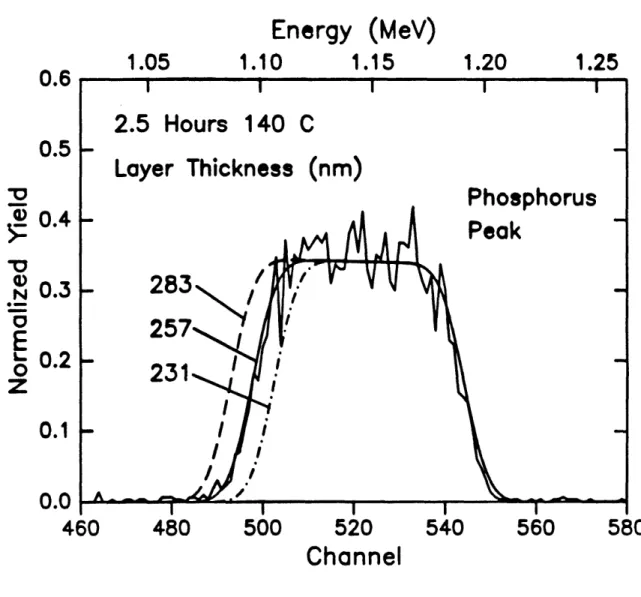
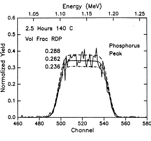
solid line is drawn for a 'simulated' sample which has a layer of material 257 rn thick which is 026 volume fraction RDP followed by an infinitely thick layer of substrate material. The parameters in the 'simulated' sample which were allowed to vary were the thickness of the mixed layer, and the volume fraction of the diffusant in that layer. Figures 6 and 7 show the sensitivity of the fits to the thickness of the 'simulated' n-dxed layer and the volume fraction RDP in the 'simulated' layer. The excellent agreement between the rough calculations discussed here and the rigorous iterative calculations performed with RUMP underscores the ability of RBS to yield quantitative results.

Energy (MeV)

0^^

0.6

0.8

1.0

1.2

400

C

0

0

200

100

0

200

300

400

500

600

Channel

Energy

1.05

_1.10

1.15

1.20

1.25

0.6

0.5

0

0

0

E

0

z

0.4

0.3

0.2

0.1

0.0

460

480

500

520

540

560

Channel

580

Figure 2.6 Sensitivity of RUMP fit to RBS data with variation of the'simulated!

penetration depth.

Energy

(MeV)

1.20

1.05

1.10

1.15

1.25

0.6

0.5

0.4

0.3

0.2

0

Y--la

0

a

E

t-o

z

0.1

0.0

460

480

500

520

540

560

Channel

580

Figure 27 Sensitivity of RUMP fit to RBS data with variation of the'simulated'RDP

2.4 Forward Recoil Spectroscopy

Many of the concepts and equations discussed in the context of RBS experiments also apply in FRES. RBS probes the volume fraction versus depth profile of medium to heavy atomic weight elements in the sample based on differences in energy and yield of backscattered particles. FRES probes the volume fraction versus depth profile of light elements, namely deuterium and hydrogen, based on differences in energy and yield of

recoiled particles. Diffusion profiles are typically determined for a deuterated species which has penetrated into a hydrogenated matrix. The configuration of the experiment is shown in figure 28.26,27

Sample

mylar

15

000010

1500

He,

H

3 MeV He

D9

H

Detector

Figure 28 Configuration of the FRES experiment.

A 3 MeV beam of alpha particles He++) is directed towards the sample at a glancing angle of 15'. Some of the incident ions are scattered from heavy elements in the sample, and another small percentage of the incident ions have collisions with deuterium and hydrogen nuclei in the smple which result in recoiled deuterium and hydrogen ions. Only the particles which are recoiled at an angle 150' from the incident beam are collected. The angle is defined by placing a slit in front of the detector which subtends a solid angle of 6.3 x 10-3 steridians. A large number of He ions are scattered from the sample at this

angle, too. A mylar foil is placed in front of the slit that is just thick enough to stop an of the scattered He ions, but will allow the smaller recoiled deuterium and hydrogen particles to pass through with some loss of energy. The thickness of the mylar is 11.5 Jim.

Deuterium and hydrogen particles are counted as a function of their energy with a detector, amplifier, and multi-channel analyzer. 'Me energy range of interest, to 2 MeV, is divided into 512 channels with approximately 4 keV/channel. Data is usually ollected for a total

beam dose 15 gC which is determined by integrating the beam current over the collection period.

A schematic of elastic collision which results in a recoiled particle at the angle of the detector is presented in figure 29.

H or D, E2

30 0

Figure 2.9 Elastic Recoil Collision in FRES.

The ratio of energies between the recoiled particle and the incident particle isi

H or D

AX

t

-4MHeMHorD Cos 2 30,

(MHe + MHo, D)" El = K =

El (2.16)

where K' is the recoil kinematic factor whose value is 048 and 067 for hydrogen and deuterium respectively. This difference in energy transfer in the elastic collisions is the reason why the deuterium and hydrogen peaks are separated in the energy spectra of a FRES experiment.

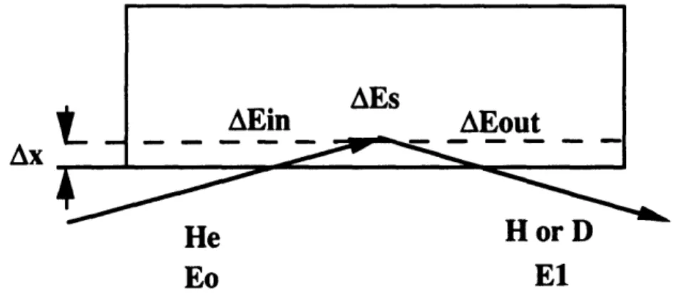
Depth profiling in FRES is most easily illustrated with an example in which energy losses are calculated along each step of a recoil event which occurs at a depth Ax in the sample. A schematic of the process is shown in figure 2 10.

AEin

AEs

AEout

He

Eo

or

El

Figure 2. 10 Schematic of recoil event in FRES.

'Me energy loss along the inward path of te incident ion, AEin is

AX dE

Min =

-sin(15') dx HeE. (2.17)

where the energy loss function is indicated by a subscript to be for a He ion. The energy of the He ion immediately before collision, Ex is

EAx = Eo - AEM (2.18)

The energy loss in the elastic collision, AEs is

AE's = - K)EAx. (2.19)

On the outward path, the energy loss is calculated for with the loss function of the recoiled particle such that

Ax (dE)

AEOUt _{= ;n(15*)} -)HorDE,' _dx (2.20)

Recoiled particles also lose energy in the mylar foil, Emylar, and the detected energy, Ed,

is found by combining equations 217 to 220 such that

Ed= Eo - E - Es - AEout - AEmylar- (2.21)

Thus the detected energy for a recoiled hydrogen or deuterium particle is a unique function of the depth in the sample from which the particle originateA

The yield of recoiled particles, either hydrogen or deuterium, is related to the scattering cross section of each element. In contrast to the RBS experiment where values of cr are tabulated and/or calculaWA the ratio of deuterium and hydrogen cross sections in the geometry of the FRES experiment are determined experimentally. 'Me ratio is assumed to remain constant in the energy range of interest. Data is ollected for a calibration sample which is 210 nm thick and is a homogeneous blend of 0277 volume fraction perdeuterated polystyrene and 0723 volume fraction hydrogenated polystyrene (figure 21 1). The ratio

densities in the sample. Since the ratio of cross sections is assumed constant in this energy range, the integrated areas under the peaks are used instead of the peak heights in equation 2.13 for improved statistical accuracy In this sample the ratio is 148. The cross sections are strong functions of the geometry of the experiment and this calibration standard is run and analyzed every time that FRES experiments are performed. 'Me calibration standard is also used to relate channel number to energy. Knowledge of the recoil kinematic factors, the incident ion energy, and the thickness of the mylar foil allows the calculation of the energies of deuterium and hydrogen recoiled from the surface of the sample. The channel numbers which correspond to these energies is found from the experimental data. A linear relationship is thus determined for energy as a function of channel number, and the

energies are indicated on the top axis of figure 21 .

(MeV)

1.4

Energy

1.2

0.8

1.0

1.6

40

30

20

10

la

0

5--la

E

L-o

z

0

100

150

200

250

Channel

300

Figurr 2.11 FRES data from a homogeneous blend of 0.277/0.723 dPS/hPS which is