The digital implementation of control compensators : the coefficient wordlength issue

October, 1979 LIDS-P-897

(revised version)

THE DIGITAL IMPLEMENTATION OF CONTROL COMPENSATORS: THE COEFFICIENT WORDLENGTH ISSUE

by

Paul Moroney

Massachusetts Institute of Technology Cambridge, Massachusetts 02139 & The Charles Stark Draper Laboratory, Inc.

555 Technology Square

Cambridge, Massachusetts 02139 Alan S. Willsky

Laboratory for Information and Decision Systems Department of Electrical Engineering and

Computer Sciences Cambridge, Massachusetts 02139

Paul K. Houpt

Laboratory for Information and Decision Systems Department of Mechanical Engineering

Massachusetts Institute of Technology Cambridge, Massachusetts 02139

ABSTRACT

There exist a number of mathematical procedures for designing discrete-time compensators. However, the digital implementation of these designs, with a microprocessor for example, has not received nearly as thorough an investigation. The finite-precision nature of the digital hardware makes it necessary to choose a computational structure that will perform adequately with regard to the initial objectives of the design. This paper describes a procedure for estimating the required fixed-point coefficient wordlength for any given computational structure for the implementation of a single-input single output LQG design. The results are compared to the actual number of bits necessary to achieve a specified performance index.

* This work was performed in part at the MIT Laboratory for Information and Decision Systems with support provided by NASA Ames under grant NGL-22-009-124 and in part at the Charles Stark Draper Laboratory.

I. INTRODUCTION

The design of discrete-time compensators through the use of optimal regulators, pole-placement concepts, observer theory, optimal filtering [1,2] and also via classical control theory [3] has received a great deal of

attention in the literature. In the past such designs have usually been implemented on large, expensive, floating-point computer systems. However, the number of applications that could effectively use small-scale hardware

control systems that work in real time has greatly increased, especially with the advent of the inexpensive microprocessor.

While the recent advances in digital hardware capabilities have opened many new possibilities for control system implementations, they have also

raised new issues. A number of these involve the problems that arise in dealing with the fixed-point arithmetic and finite wordlengths of small-scale digital systems. As these problems are not addressed at all in the idealized mathematical design procedures that have been developed to date, a methodology must be established for treating the digital implementation of a design.

The mathematical design procedure produces an infinite-precision ideal compensator specification. The job of the implementation step is to

specify and order sequentially the critical computations that must take place in the compensator so that the end result, the actual finite-precision

digital system, performs as close to the ideal as is consistent with the expense and speed requirements of the application. The implementation step also includes a specification of the hardware architecture and components.

-2-phases may not be totally independent, since the implementation can be very

important in determining an acceptable sampling rate and the number of

operations that can be performed per sampling period. These then become

restrictions on the compensator design.

Our approach draws on the field of digital signal processing [4,5],

which has generated many results concerning the realistic implementation

of digital filters. Good reviews concerning.the effects of finite precision

in digital filters - specifically, the effects of coefficient quantization,

limit cycles, and quantization noise - can be found in [6],[7] and [8].

Some work has been done in looking at similar questions for digital

feedback compensators, but it has been somewhat limited. Knowles and

Edwards [9] and Curry [103 have each considered a roundoff noise analysis

of certain sampled-data systems. Bertram [11], Slaughter [12], Johnson [13],

and Lack [14] have developed amplitude bounds on the. effects of quantization

in sampled-data control systems. Sripad [15] has looked in some depth at

the roundoff noise and finite-precision coefficient performance of the

discrete-time lalman filter and linear-quadratic-Gaussian controller. Rink and Chong

[161 have derived bounds on the effects of quantization errors in

floating-point regulators. Farrar [17] has floating-pointed out in a basic way some of the

issues involved in implementing continuous-time linear-quadratic-Gaussian

controllers as discrete-time fixed-point microprocessor-based systems,

Willsky [18] has pointed out some of the parallels between filter and controller

implementations. In this paper, we use, adapt, and extend the ideas

-3-we examine the issue of coefficient quantization in fixed-point compen-sator implementations. Since researchers in digital signal processing have developed a great many tools for implementing digital filters, we should try to use these concepts. However, because of the presence of a feedback loop around the digital compensator, many of these concepts do not directly apply for control, and adaptations are necessary. Finally, in our

treatment, where the coefficients of the ideal compensator have been chosen to optimize some scalar criterion, we have to modify the notion of

statistical coefficient wordlength. This modification also constitutes a possible extension for digital signal processing.

The basic idea behind the selection of a coefficient wordlength is the

same for digital filters and digital compensators. Approximating the coefficients of a structure with a finite number of bits causes a degra-dation in the system's performance as compared to the ideal. Assuming that a given quantitative performance measure is provided, we can measure the tradeoff in the number of bits vs. the degradation. Then, assuming that we specify an acceptable amount of degradation, one must determine the minimum number of coefficient bits needed to meet this goal. Clearly a straight-forward way to determine this wordlength is to simply reevaluate the measure of performance for sets of coefficients that are quantized to different wordlengths, and to choose the smallest wordlength meeting the design

spe-cification. This direct method can be quite tire-consuming, even when we assume that the coefficients are to be rounded to the shorter wordlengths, and not choosen in some more complex fashion [19,.

-4-The concept of a (simpler) statistical estimate of the wordlength

originated in the study of digital filters with the work of Knowles and

Olcayto [20]. Avenhaus [19] applied this idea to the digital filter power

transfer function (as a performance measure), and later Crochiere (21,22]

used the concept with the filter transfer function magnitude and a wordlength

optimization procedure. All three of these studies chose different performance

measures, none of which seem to be particularly appropriate for control problems

where the compensator phase is critical. In this paper we adapt the

statistical wordlength concept to the steady-state linear-quadratic-Gaussian

(L_QG) control problem. We have selected the LQG problem for several reasons,

First, it has received a great deal of attention in the recent literature,

due to its robustness, multivariate formulation, and optimal nature. Second,

the LQG problem has an explicit scalar performance index, J, which can be used

to gauge the effectiveness of an implementation. In fact, this was the

performance measure used by Sripad [15]3

It would also have been possible to choose a criterion such as phase

margin, output noise power, or any combination of stability Or noise measures,

If the problem under consideration was simply a Kalman filter, then a

suitable performance measure would be the trace of the error covariance matrix.

We have chosen J in order to present our results in a specific context.,

These results extend in a straighforward manner to other measures. It should

also be noted that we treat the single-input single-output case for

convenience, and because it is in this setting that most digital filtering

resiultgs have been developed. The following analysis can be extended easily

to the input output case, once a input

-5-In terms of its applications, the statistical wordlength estimate that vwe develop is useful in the relative comparison of different structures

on the basis of their required coefficient wordlengths. However, more

importantly, the statistical estimate can be used as the basis for an iterative gradient-search constrained optimization procedure (see [23] and the conclusions of this paper) for generating minimum coefficient wordlength structures. This is possible because the statistical estimate is continuous, that is, not

limited to an integral number of bits and also because this estimate is differentiable with respect to the coefficients of the structure. These

points are not true of the direct method of wordlength determination, which is essentially the method used by Sripad [15].

The organization of this paper is as follows: in Section 2 we

describe the derivation of the LQG compensator including the real computation time constraints. The notion of a compensator structure and a notation adequate for expressing the computations that occur in such a structure is presented in section 3. In sections 4,5 and 6 we introduce the notion of statistical wordlength and apply it to the LQG problem. Finally, we

present examples of the technique and compare the results to the direct method.

2. THE LQG CONTROLLER PROBLEM

In this section we present the single-input single-output LQG

control configuration and the mathematical, or ideal, design of the compensator. Assume that we wish to design a digital discrete-time compensator for a

constant. Typically, after sampling the plant output at rate - , the

compensator is designed to produce an output u(k) based on the compensator inputs up to and including y(k). Such a design would not be implementable, since u(k) and y(k) refer to identical sample times, and a finite time must be allowed for the computation of u(k) from y(k). These two requirements are contradictory.

Kwakernaak and Sivan [1] present a design procedure where u(k) depends only on compensator inputs up to and including y(k-l). Thus allows a full sample interval for the computation of u(k). If however, the computation time is much shorter than the sample interval, this implies some inefficiency; the output u(k) will be available long before it is used as a control. Thus Kwakernaak and Sivan also include a method for skewing the sample time of the plant output with respect to the rest of the compensator. The compensator output u(k) will still depend on input up to and including y(k-l), but now y(k-l) is produced only one calculation time before u(k) is needed. This eliminates any inefficiency. [1,23].

When we discretize the continuous-time plant model at some rate 1/T and account for any sample skewing we obtain the following set of equations describing the plant output at the sample times:

x(k+l) = fx(k) + ru(k) + w_l(k)

(1) y(k) = Lx(k) + w2(k)

where n is the system order, i(nxn) is the transition matrix, r(nxl) and L(lxn) are the input and output gains, and wl and w₂ are discrete white

-7-Gaussian noise sequences with covariance matrices Q1(nxn) and 02(1xl)

respectively. The control law is chosen to minimize the following performance

index: (the discretized version of a continuous-time performance index)

E lir (X' (k)Qx(k)42x'(k)Mu(k)+Ru2 (k)) (2) 2i

ix0 k=-i

where Q is nxn, M is nxl, and R is lxl. Assuming a piecewise-constant control

signal u(t) formed by applying the u(k) samples to a zero-order hold, and a

linear compensator, the optimal compensator design can be described as follows:

x(k+l) = b(k) + ru(k) + K(y(k) - Lx(k))

(3)

u(k+l) = Gx(k+l)

Note that the equations in (3) base the current control u(k) only on

past outputs y(k-l), y(k-2),...,[1], as discussed above. The (nxl) matrix

K is the solution to a Kalman filter problem, and can be computed by solving

the following algebraic Ricatti equation: [11

X = - EL' (. +LEL') 1L} ' +

01

(4) where K = ELL' ( 2+LEL ')

Similarly, the (lxn) matrix G results from an optimal regulator design and

the following algebraic Riccati equation [1].

P= (T-rR M,)'P{I-r(R+rl,P ) r'P}(z-rR 1 M') + Q-MR -M' -where G = (R+-1M'

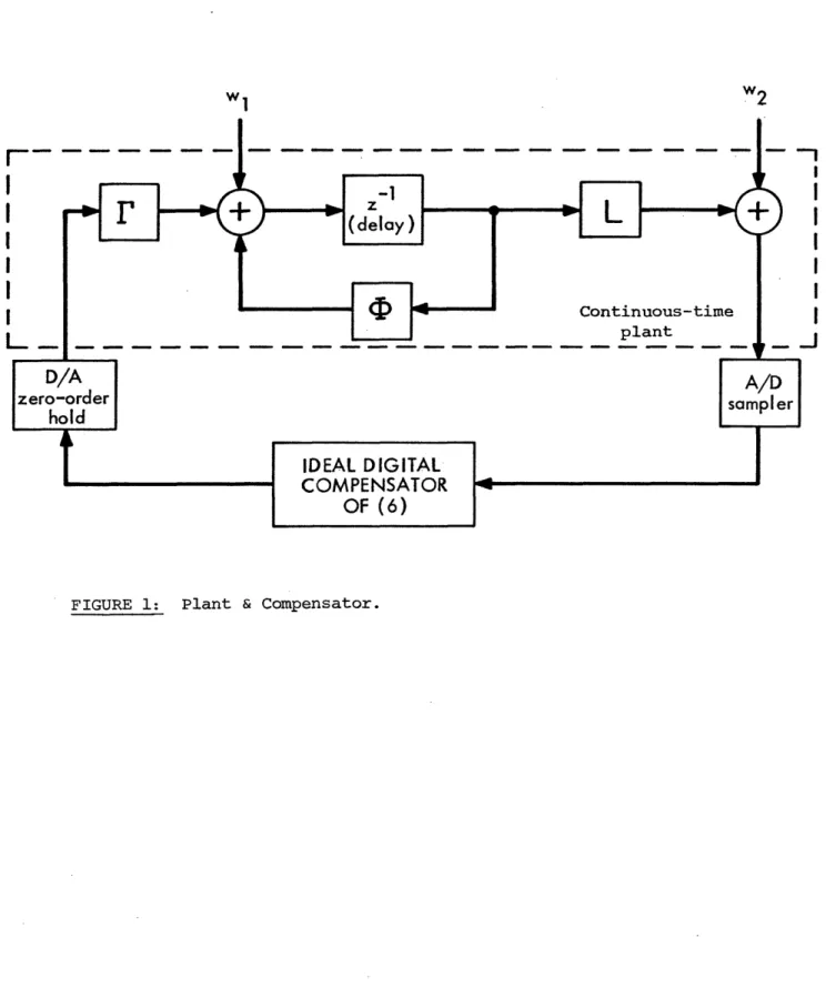
Figure 1 presents a simple block diagram of the system and its

(infinite-precision) compensator. This ideal compensator (3) can be described

by an infinite-precision map (transfer function) in the digital frequency

domain:

U(z) = -G(z - t+KL + rG) K (6)

Y (z)

The digital filter transfer function (6) must be implemented in finite precision and therefore will suffer some degradation in the system's measure of performance J.

3. ALGORITHMS AND STRUCTURES

In order to discuss different implementations, one must have an accurate

notation that reflects these differences. The term 'structure' is

employed to specify the exact finite-precision algorithm by which the

compen-sator output samples u are generated from its input samples y. All structures

for implementing a given filter or compensator would perform identically under

infinite-precision arithmetic, but produce different quantization noise,

coefficient quantization effects, and limit cycles when implemented in

finite-precision, A good review of some of the structure used to implement

single-input, single output digital filters can be found in [22], [24] and [25].

Now let us examine the compensator equations (3) to see if they represent

a possible computational structure. Consider the states x(k) to be the

states of the structure, where a state corresponds to the output of a delay

element in the signal flow graph [223 of the structure. Then the x(k+l)

equation describes the new state values to be functions of the current states

!1 "2

I~~~~~W

Z1

(delay)

j

Continuous-time

~~~~~L

__ _

~~~~~~plant

D/A

_A/E

zero-order

_hold

samplr

IDEAL DIGITAL

COMPENSATOR

OF (6)

-9-is an accurate representation of a set of computations. However, the last

equation in (3) shows the next output value to be a function of the next

state values. This cannot accurately describe real computations, since some

finite time must be allowed to compute u(k+l) from x(k+l), and this is inconsistent

with the identical (k+l) indices. There is in effect a series delay that is

implied, yet such a delay is not accounted for in the compensator design.

This example points out the difference between compensator and filter

structures [23]. _{In digital filtering, (3) would be taken to represent a}

structure. This is done frequently in describing the dependence of the output

node on the state nodes. The series delay that must exist is ignored; after

all, series delay in the filter output is not really important. However, in

control systems, series delay is critical. Unplanned for delay adds negative

phase shift and affects the performance of the closed-loop system in a

negative way, Thus we must include all the required computational delays in

our description of a compensator structure, Simply adding the delay to the

plant model and redesigning the compensator is a poor solution, since the

order of the cqmpensator will increase when we do this. The best solution is

to i4rpjement the compensator in such a way that its computations can take

place in the allotted time intervals. For example, we can rewrite (3) as

follows;

X(k+X? J = ( rT (X) + + Ku((yk) (k) )

(7) u(k~l) -i-G{ i(k) + Fu(k) + K(y(k)-I(k))

The, equations (7) do represent a compensator struqture, since the next values

-10-fact, note that u(k), the compensator output, is a state. This will always

be true for compensator structures. For any n -order filter structure with

only n unit delays (canonic in delays), a corresponding nth -order compensator

structure will exist. However, the LQG compensator structure will have an

extra delay at its output because of the series delay. Thus, an n -order

delay-canonic compensator structure will have n+l unit delay elements.

Since the notion of a compensator structure is thus different from a

filter structure, we must adapt the filter structure notation to account for

the differences. Let u and y represent the compensator output and input

respectively. Let v represent the compensator states (other than u). We

can adapt the notation used by Chan [24] for digital filters to produce the

following: modified state space representation: [23]'.

=-I O+l) _(k)

Several important points mak~e (8) use.ft!;

(1) Each (roQunded) coefficient in the structure occurs, once and only

once as an entry in one of the .i matrices. The re.mainder of the matrix

entries are ones and zeros.

(2) T'he concept of a precedence. to the operations (muntiplies, ads, an,

quantizations) is maintained. The ordering of the

'

matrices implies'that the operations in computing the intermediate nodes

v(k)

rl = u(1k)

E

are completed first, then y(k)

r2 =2

[(

]k)j

next, and so forth. The para

meter q specifies the number of such precedence levels. Examples of the

modified state space representation appear in Section 7.

Notationally, it is also useful to define %V to be the infinite precision product of T Tq- 1' '....'y and to partition it as follows:

Too = [11 T 121 (9)

where 11 is (n+l) by (n+l) and T!2 is (n+l) by 1.

4. STATISTICAL WORDLENGTH FOR DIGITAL FILTERS

In this section we review briefly the basic development of the

statistical wordlength measure as used in digital signal processing [21].

Consider a general measure of performance f, a differentiable function of the

coefficients (cl,c₂,.. ,c ) of the structure. The value of f associated with

any particular finite-precision structure reflects a degradation in

performance as compared to the ideal (unrounded coefficients) case fa. This

degradation df can be expanded in a Taylor's series about the ideal value.

-12-df(ClC i dc. (10) 1 2 ' m 1ci i i=l 00 th

where c. is the i coefficient to be rounded, dc. is the error due to I1

quantization, and

af

is the first partial derivative of f evaluated at 1

00

the unrounded coefficient values. Note that coefficients such as 3,2,1, .

are not normally affected by rounding and should not be included in the sum

(10).

If A is the quantization step size (the fraction represented by the

least significant bit of the fixed-point coefficient word), then each dci

must lie between + - (rounding assumed). Given the partial derivatives in

(10), we could (upper) bound the error df, producing a very pessimistic

wordlength estimate. Specifically,

2 Dl aci (ll)

i=l(

The basic statistical wordlength idea is to produce a less pessimistic

estimate by treating an ensemble of structures. Over this ensemble, the

coefficient errors dc.i can be thought of as uniformly-distributed zero-mean

uncorrelated random variables, each of variance A 2/12. Using (10), we can

now treat df as a random variable. With dci as described above, df will

-13-2 a2 m 2

2~ A~-

Z

f (12)

'df 12 i ci (12)

For large m, the central limit theorem can then be applied to justify

a Gaussian distribution for df. Thus with a given confidence level

(probability), say 95%, one can predict the variance cdf needed for the

error df to remain within some prescribed bound. In other words, 95 out of

100 of the structures in the ensemble will result in systems where df remains

within this bound.

From a table of the Gaussian distribution,

Pr[ dfl 2

df

.954 (13)

If the quantity of interest f is constrained to lie within + E of the

-0

ideal f , then (13) implies that adf equal Eo/2. This result can be combined with (12) to produce an estimate of the parameter A:

A o (14)

i=l

)

Given A, the statistical wordlength can be defined to be

SW5L = + og₂ (15)

The first term in (11) represents the number of bits necessary to

represent the integer portion of the coefficients and the second term gives

the number of bits necessary for the fractional portion of the coefficient

-14-Crochiere [21,22,25] has presented a number of results comparing the

statistical wordlength of structures, using the transfer function magnitude

as the performance measure f. Since this choice of f is frequency-dependent,

the resulting estimate is also frequency-dependent. The final wordlength

can be selected as the maximum of the estimates over the frequency range

of interest. In the examples treated by Crochiere, the statistical wordlength

estimate was typically 1 to 3 bits conservative as compared to the actual

minimum number of bits necessary to meet the transfer function error limit.

Using the statistical wordlength idea, Crochiere [21] was also able to

for-mulate an optimization procedure for designing, shorter-coefficient-wordlength

filter structures. Although this optimization method is quite different from

the one we have alluded to it is a big motivation for developing the

statistical approach for compensators.

5. STATISTICAL WQORDLENGTH AND THE PERFORMANCE INDEX J

As mentioned in section 2, it is Qonvenient to use the performance index

J in (2) as the measure of performance f in an LQG setting. Using the approach

of the previous section, the change in J would be estimated by:

d ) (C1,q2'-* ne E 3ci | dc. (16)

However, the optimxal nature of the LQG control problem forces all the

sens'it;ivities

Di

to be zero, Therefore a higher-order approximation

is necessary:

dj

2 3 c, acc{ 1 dc.dc, (17)

2i3 j-q. C D j

-15-The use of second-order terms (not used in digital filter analysis) is

a unique aspect of our statistical wordlength formulation. However, the use

of these terms would be necessary in any filter or compensator design analysis

in which the statistical estimate is based on the degradation in a scalar

performance measure that has been optimized with respect to the unrounded

coefficients. For example, if a digital filter were designed by minimizing

the integrated squared error between the desired and actual filter transfer

function magnitude characteristics, then a statistical wordlength estimate

based on this performance measure would have to use second-order sensitivities,

since all first-order sensitivities would be zero. The statistical wordlength

derivation that we have developed would have to be used in this case, and

therefore our formulation also has some potential applications in digital

filter design.

Proceeding from (17), the mean of dJ will no longer be zero:

E(dJ) =

(

)E[dc2 (18)

2i=l c_i

For convenience, define the random variable e to be the square of dc..

Its mean and variance can be shown to be A 2/12 and A 4/180. The variance

of dJ can now be found (23]:

2 =2 2

\2 +(D(19)

i=! ~ ~c_i { i=l j=l

Dcic

_j

-16-Recall the application of the central limit theorem in section 4. We

can make the same assumption for our higher-order statistical wordlength

derivation. For the usual digital filtering estimate, the coefficient

quantization could either decrease or increase the error in the transfer

function magnitude at any specific frequency. This implied that the error

was zero-mean. In the control case, the value of J can only increase under

coefficient quantization. Thus we need only have a specification on the

maximum allowed value of J including the degradation due to coefficient quant-ization: J+E Following the general approach of section 4, we must equate

this value to the two-sigma point in the distribution for dJ in order to

compute our estimate of A:

J +E = J + dJ + 2Cdj (20)

This choice of adJ gives a 97.5% confidence level in terms of remaining

below the allowed deviation E . Combining (19) and (20) we can derive an

expression for A2:

2-~

~

2 1 1 m ~2 m 2 j 1 1 |m- m| + _) 2 2 o i j=l ( c.j ) 1 i=l ac 2 i<j 00 (21) 24E o i=l c.

Using (15), the SWL can then be written:

SWL = + _{2 log}log2 (22)

p(dJ)

JF

a

_·

i

Joo+dJ

Joo+Eo

-17-The use of second-partial derivatives in approximating dJ in (17) has given rise to a complex expression for the statistical wordlength. Efficient methods for evaluating (22) will be discussed in the next section.

6. COMPUTATIONAL PROCEDURE

In order to compute the derivates of Jo, the infinite-precision (ideal) performance index, it is convenient to use the trace form [26] of equation

(2):

JO = trace [S Z] (23)

where the (2n+l)x(2n+l) matrices S and Z are defined by (24) and (25):

0 ' M S - ____----1 __ S= I= O' ' (24) J j Z = E [x (k) [x'(k),vu'(k),u(k)] (25) v (k)

Here Q, M, and R are the performance index parameters described in (2). The matrix Z, the covariance matrix for plant and compensator states, can be shown to satisfy the following Lyapunov equation:

Z = AZA' + [01 1 (26)

-18-where

,' 0 ,

A = ! (27)

12

'

11

Note that (23)-(26) depend on the infinite-precision (ideal) compensator and

on the selection of componesator state variables v. The resulting JX will be

independent of structure. However, the partial derivatives of Jc, (evaluated

for ideal coefficients) will depend on the structure since each coefficient

Ci. resides in one of the structure's T. matrices. Taking the partial

derivatives of (23) will produce:

,2 2

ac

c

= trace S icj (28)

where all the partials in (28) are evaluated at the ideal values of the

coefficients.

Thus we must compute the second partials of Z. Taking the first

derivative of (22) produces: = A A' + Qi + Qi (29) i i where 0 0 Qi -a 0c 12 Dc, 0212

Evaluation of the trace expression in (28) will imply solving m Lyapunov

-19-we must take the derivative of (29) with respect to c.: [23]

2 2z = A A' + Xij + X. (30) Dcjac DCAC

J1

1 where DA DZ DA 9Z AA' D2A2A X. A' + A' + + ZA'

13 acj ac c. c. ac. ac--. c.c.

0

1

!2 112 D2a12

0C +

S

Q0 2

aC.

02 12

m (m+l)

Solving (30) for all i and j would require ) more Lyapunov solutions;

this would be extremely time-consuming.

Fortunately, this burden can be substantially reduced. Specifically,

the concept of adjoint operators [1,23] can be used to simplify (28) and

(30). The expression in (28) can be replaced by:

a2J

DDc. = 2 trace (UX..) - (31)

Where U satisfies U-A'UA=S. Thus we need to solve this one Lyapunov equation

plus the m equations in (29) in order to compute the X... This saves 1]

solving the m(m+l) equations of (30). 2

-20-There is still the problem of the m Lyapunov solutions needed for the derivatives aZ/ac. used in X... By using the Lyapunov solution method of Barraud [27), these computations can also be simplified. Consider the general

Lyapunov equation (32):

X = FXF' + C (32)

Barraud's method breaks into two distinct parts, one which transforms F

into the upper Schur form, and one which back substitutes using the transformed F and C matrices. The major portion of this computation involves the initial F transformation. Thus, if there exist several Lyapunov equations with

identical F matrices but different C matrices, then the F transformation need be done only once. This is exactly the situation for the Lyapunov equations

(26) and (29) needed for X... Typically, more than 75% of the Lyapunov computation time can be saved, depending on the particular A matrix.

Still further computational time savings are possible. A more complete description of the computational procedure is available in [23].

7. AN LQG EXAMPLE

A sixth-order example was chosen to test the statistical wordlength algorithm. It was adapted from the longitudinal control system design done for the F8 digital fly-by-wire fighter [28). The continuous-time plant parameters and performance index parameters are given below:

-21-Continuous Time System Parameters:

-4 -0.6696 5.7x10 -9.01 0 -15.77 0 0 -0.01357 -14.11 -32.2 -0.433 0 A= 1 -1.2xl0- 4 -1.214 0 -0.1394 0 1 0 0 0 0 0 0 0 0 0 -12 12 0 0 0 0 0 0 B = [0 0 0 0 0 0 1] C = [1 0.003091 31.28 1 3.592 0]

Continuous-Time Performance Index Parameter:

6.637 0 0 0 0 0 -7 -3 -4 Q = 0 2.6554x10 2.686x10 0 3.085xlO 0 -3 0 2.686x0l 27.174 0 3.121 0 0 0 0 27.174 0 0 -4 0 3.085x10 3.121 0 0.3585 0 0 0 0 0 0 0 R = 5.252

Continuous-Time Noise Covariances

= diag0 0 0 0 10- 6 10 -6]

-22-This continuous-time system was discretized at a sample rate of 10 Hz and the optimal regulator and Kalman filter designed. The double-precision parameters

1,

r, L, Q, M, R, 01' 02' G, and K can be found in [23].

Five structures for implementing the ideal compensator transfer function (6) were examined. These were the digital filtering-based direct form II structure, a cascade of direct form II second-order sections, a parallel structure composed of such sections, a block-optimal minimum roundoff noise structure, and the structure described in (7) which we have called the simple structure. In all five cases we present the initial design coefficient values. These are not typically the coefficients that are used however; if

they were used the structures could exhibit overflows. Consequently, we apply a scaling procedure that we have adapted for compensators [23] from the Z2 scaling of digital filters [29]. In any case where a unity entry in the unscaled structure would become a multiplier coefficient (non-unity, non-power of two) when scaled, we have indicated this with an asterisk.

The first structure we examine is the direct form II. Figure 3 presents its signal flow graph. Note the presence of the delay preceding

the output node: The 12 coefficients of the direct form II structure come directly from the unfactored transfer function (33), and its modified state space representation (two precedence levels) is shown in (34).

-1 -2 -3 -4 -5 -6

alz +a2z a z +a3z +a z +a6z

H(z) = 3 -4 -5 -6 (33)

l+bz +b 2z +b 3 +b z +b z +b 6z

a,

zI

- Z-I

b

Z

tZ

!

-23-1 0 0 0 0 0 0 1 0 0 0 0 O 0 1 0 0 0 T2 1 0 0 0 1 0 0 O O 0 0 1 0

o

0 0 0 0 1 (34) a₆ a₅ a₄ a3 2 a 0 1 0 0 0 0 0 0 O 0 1 0 0 0 0 0 O .0 0 1 0 0 0 0 O O 0 0 1 0 0 0 O O O0 0 1 0 0 -b -b₅ -b -b₃ -b2 -bl O 1*

When this structure is k2 scaled, the unity valued marked with an asterisk

becomes a 13thon-unity coefficient.

The second structure, the cascade, derives its coefficients from a

multiplicative factorization (and there are several ways to group the poles

and zeros [23]) of (33) and breaks into 3 series direct form II second-order

sections. The factored transfer function is shown in (35). This structure

has 12 coefficients, 4 precedence levels, and requires 3 additional

-24-(dlz +d2z ) (l Z +dz )(l+dz +d6Z-2 H(z) _{1(z) = ( -1} 2 _{-21 -2 -1 -2} (35) (1 +C+cz +Cz ) (+cz +c z )(i+cz -1+c z- 2 0 1 o 0 0 0 0 1 0 0 0 0 0 0 4 0 0 0 1 0 0 0 O 0 1 0 0 0 0 O O 0 0 0 1 0 O 0 0 0 0 0 1 O O 0 0 d6 d5 1' 1 0 0 0 0 0 0 o 1 0 0 0 0 0 O O 0 0 0 0 1 (36) 3 =

o

0 0 1 0 0 0 0o O 0 1 0 0

o

0 0 0 0 1 0 0 d0 4 d3 -C6 -c 5 1 O 0 0 0 0 1 1 0 0 0 0 0 T

~

0 I 0 0 0 0 2 0 0 1 0 0 0 0 0 0 1 0 0 0 0 0 0 1 0 d2 -c4 -c3 0 0 d

-25-o

0 i 0 0 0 0 0 0 0 1 0 0 0 0 0 T = 0 0 0 1 0 0 0 0 O 0 Q 0 1 0 0 0

o

O Q 0 0 1 0 0 -C2 -C O O 0 0 0 1*

The third structure, the, parallel form, corresponds to a

partial-fraction expansion of (33) and is divided into 5 parallel direct form II

first and second-order sections. The expanded transfer function (also

12 coefficients before scaling) is shown in (37), and its modified state

space is given in (38):

-1 -2 -1 -! -1

e z +e2 z e3z e4z e5z

.~'(z) = 'J' + + + -1 -2 -- -1 -1 l+c2z +c2z l+d3z l+d4z ! +d5z

~~~-1 ~(37)

-1 e6z l+d z 1 0 0 0 0 0 0 1 0 0 0 0 O 0 1 0 0 0 T2 = I 1 (38) 0 0 0 1 0 0 0 0 0 0 1 0 0 0 0 0 0 1 e e e e e e 2 1 3 4 5 6

-26-0 1 0 0 0 0 0 0 -C2 -c1 0 0 0 0 0 1* 1 O 0 -C3 0 0 0 0 1* O 0 0 -C₄ 0 0 0 1* O 0 0 0 -C₅ 0 0 1* O 0 0 0 0 -c6 0 1*

To scale this structure, 5 additional scalers (one per section) are

required [23].

The fourth structure tested was a parallel block optimal minimum

roundoff noise structure analogous to the minimum roundoff noise filter

structure discussed by Mullis and Roberts [29]and Hwang [30]. However,

since the roundoff noise performance of a LQG control system depends on the

overall closed-loop behavior, it was also necessary to adapt the techniques

of Mullis and Roberts and Hwang for compensators[23]. This structure is

reported to have low coefficient sensitivity when used as a filter even

though it requires 25 coefficients, which is many more than the previous

three structures. The modified state space is shown in (39), and has 3

-27-fl f2 0 0 0 0 0 f f4 f5 0 0 0 0 0 f Y,1 = (39) 0 0 f7 f 0 0 0 f 0 0 f10 f 0 0 0 f12 0 0 0 0 f13 f4 0 f1 0 0 0 0 f16 7 f18 f19 f20 f21 f22 f23 f24 0 f25

The last structure, the simple structure, is taken directly from the

LQG compensator equations (7). In other words those equations exactly

describe the computations that must take place. The parameters of

a,

r, K, L, and G are taken to be the coefficient values of the structure (before scaling). We have considered this structure because it has been

used to implement LQG compensators more or less by default. The form of

the transfer function containing the coefficients of this structure is that

of (6), and the modified state space is shown below:

3

T TX

FlL1

- -

_-__F..I_

(40)

I 0 '1 -L , 0 !i

Note the three precedence levels, and also the enormous number of

-28-Table 1 presents data comparing the statistical wordlength estimates of the five structures mentioned above to the actual required wordlength as

computed by the direct, almost trial-and-error, approach mentioned in section 1. This actual value is called the 'TWL' (true wordlength) in Table 1, and was computed using a modified binary search algorithm [23]. The amount of com-putation time required for each SWL or TWL calculation is also included in parentheses.

For the system tested, a five per cent degradation was specified as the maximum allowed deterioration in the measure of performance J. The wordlength values presented in Table 1 do not include a sign bit.

Structure SWL bits TWL bits Coefficients

(eqns.1) (time) (time) (incl. scaling multiplies)

direct-II 16 35.99(.81) 32(1.2) 13 (33,34) cascade 6 14.61(.86) 14(1.36) 15 (35,36) parallel 1 6.84(.93) 6(1.08) 17 (37,38) block optimal 1 7.02(1.26) 7(1.11) 25 (39) simple 1 9.05(2.44) 9(1.71) 50 (6,40)

TABLE 1: $WL Results for the F8 Example.

The effect of structure on coefficient wordlength is evident from Table 1. For compensators, the most important observation to make is that although the simple structure performs fairly well in terms of its required coefficient wordlength, it is inefficient. It requires far too

-29-many multipliers compared to the parallel direct form II and parallel block

optimal structures which also outperform it. Yet this structure has been

commonly used.

Among the remaining structures shown, the direct form II requires the

most bits by far, as is typical of digital filter applications [4]. The

best structure of the 5 is clearly the parallel direct form II, requiring

6 bit words and 17 coefficients. In performance, the block optimal is

nearly as good; however it requires 8 extra coefficients,

As an estimate, the SWL was from 0.02 to 0.84 bits conservative for

the best four structures, which is extremely good, but 3.99 bits conservative

for the direct form II. As a comparison, recall the digital filter results

of Crochiere [22], in which the SWWL, based on transfer function magnitude,

was 1 to 3 bits conservative, In terms of execution time, the SWL exhibits a strong dependence on the number of coefficients in the structure. These

times can be compared to the execution times for the TWL value, which should

be relatively independent of the number of coefficients. Thus the SWL is

faster to compute. when there are fewer than 20 coefficients, and slower to

compute for more than 20, However, keep in mind that its main application is

for the. optimization of structures, where the TWL cannot be used in the same fashion.

8. CONCLUSIONS

This paper constitutes an attempt to examine the issues involved in the

digital implementation of control compensators. To deal with these issues,

we have sought to ally the fields of digital signal processing and control

-30-More specifically, this paper treats the statistical coefficient

word-length issue for the LQG compensator using fixed-point arithmetic. After

reviewing the LQG design procedure and defining the notion of an

implemen-tation structure, the statistical wordlength concept for digital filters

was described. In adapting this concept to a control and estimation problem,

the index J was chosen although the method readily extends to other measures

(.for example, the covariance matrix trace for Kalman filter problems).

Finally an efficient computational method was discussed and an illustrative

example presented,

Our results demonstrate the feasibility of using the statistical

ap-proach, in determining a sufficient LQG compensator coefficient wordlength.

One application of this technique would be in the comparison of different

structures for implementing a design. In addition, the statistical wordlength

can also be an accurate criterion for selecting the wordlength once a

specific structure is chosen.

Of more importance, the continuous nature and analytical form of the

statistical wordlength estimate (it is not confined to an integral number

of bits,) makes it possible to synthesize minimum coefficient wordlength

structuresin a straightforward manner, This would be extremely difficult

and time-consuming with the non-differentiable integer TWL. Using the.

statistical wordlength as described in section 4, Chan [24] has presented

a constrained optimization technique for digital filter design based on

continuous transformations of an initial filter structure, Given a set of

-31-used to iteratively produce structures of lower and lower coefficient

sensitivity, and thus smaller coefficient wordlengths. This idea has been

adapted for the LQG compensator statistical wordlength estimate presented

in this paper [23].

In addition, by computing the SWL estimate, we have available the

various coefficient sensitivities

a2J/ac.ac

. By examining their relative values, we can determine the dominant sensitivities in the structure. This

information can be exploited to direct any effort at optimizing wordlength

[23] or specializing the hardware multiplier associatedwith any particular

coefficient. Thus we could optimize just one portion of a higher-order

structure, instead of the entire structure. This would save on the number

of multiplies. Also, an examination of the different sensitivities opens

up the possibility of using different wordlengths in different parts of

the structure.

Other applications of the statistical coefficient wordlength estimate

developed in this paper exist. As mentioned in section 5, this statistical

procedure. including second-order sensitivities can be used for digital

filters that are designed through the optimization of some scalar criterion.

FurthermoQre, in the control field, this statistical wordlength formulation

would apply almost unchanged to suboptimal compensators designed via some

parameter optimization approach. The need for second-order sensitivities

would still exis-t.

As a final point, it should be mentioned that most of our development

applies unchanged to multiple-input multiple-output compensators 123]. The

difficulty there is in defining just how one develops structures for such

com-pensators. However, given such a structure, we can easily compute its

-32-REFERENCES

[1] H. Kwakernaak and R. Sivan, Linear Optimal Control Systems, J. Wiley & Sons, New York, 1972.

[2] M. Athans, Guest Ed., IEEE Transactions Aut. Control, Special Issue on Linear-Quadratic-Gaussian Problem, Vol. AC-16, No. 6, December 1971. [3] B.C. Kuo, Analysis and Synthesis of Sampled-Data Control Systems,

Prentice-Hall, E.nglewood Cliffs, New Jersey, 1963.

[4] A.V. Oppenheim and R.W. Schafer, Digital Signal Processing, Prentice-Hall, Englewood Cliffs, New Jersey, 1975.

[5] L.R. Rabiner and B. Gold, Theory and Application of Digital Signal Processing, Prentice-Hall, Inc., Englewood Cliffs, New Jersey, 1975. [6] T.A.C.M. Claasen, W.FG. Mecklenbrauker, and J.B.H. Peek, "Effects of

Quantization and Overflow in Recursive Digital Filters," IEEE Trans. Acoustic, Speech, and Sig. Processing, V. ASSP-24, No. 6, Dec. 1976, pp. 517-529.

[7] J.FF K"aiser, 'On the Limit Cycle Problem," Proc. IEEE Inter. Conf. Acoustics, Speech and Sig. Processing, 1976, pp. 642-644.

[8] A.V. Oppenheim and C.J. Weinstein, "Effects of Finite Register Length in Digital Filtering and the Fast Fourier Transform," Proc. IEEE, V. 60, August 1972, pp. 957-976.

[9] J,a. Knowles and R. Edwards, "Effect of a Finite-Word-Length Computer in Sampled-Data Feedback Systems," Proc. IEE, V. 112, No. 6, June 1965, pp. 1197-1207.

[10] E.E. Curry, "The Analysis of Round-Off and Truncation Errors in a Hybrid Control System," IEEE Trans. on Aut. Control, Vol. AC-13, October 1967, pp. 601-604.

[11] J.E. Bertram, "The Effect of Quantization in Sampled-Feedback systems," Trans. Amer. Inst. Elec. Engrs., Vol. 77, Pt. 2, September 1958,

pp. 177-182.

[12] J.B. Slaughter, "Quantization Errors in Digital Control Systems," IEEE Trans. Aut. Control, Vol. AC-9, No, 1, January 1964, pp. 70-74.

[13] G.W. Johnson, "Upper Bound on Dynamic Quantization Error in Digital Control Systems via the Direct Method of Lyapunov," IEEE Trans. Aut. Control, Vol. AC-10, No. 4, October 1965, pp. 439-448.

-33-[14] G.N.T. Lack and G.W. Johnson, "Comments on "Upper Bound on Dynamic Quantization Error in Digital Control Systems Via the Direct Method

of Lyapunov," IEEE Trans. Aut. Control, Vol. AC-11, April 1966, pp. 331-334.

[15] A.B. Sripad, "Models for Finite Precision Arithmetic, with Application to the Digital Implementation of Kalman Filters," Sc.D. Dissertation, Washington Univ., Sever Institute, Jan. 1978.

[16] R.E. Rink and H.Y. Chong, "Performance of State Regulator Systems with Floating-Point Computation," IEEE Trans. on Aut. Cont., V. AC-24, No. 3, June 1979, pp. 411-421.

[17] F.A. Farrar, "Microprocessor Implementation of Advanced Control Modes," Summer Computer Simulation Conference Proceedings, Chicago, Illinois, July 1977, pp. 339-342.

[18] A.S. Willsky, Digital Signal Processing and Control and Estimation Theory - Points of Tangency, Areas of Intersection, and Parallel Directions, The M.I.T. Press,' Cambridge, Mass., 1979.

[19] E. Avenhaus, "On the Design of Digital Filters with Coefficients of Limited Word Length," IEEE Trans. Audio & Electroaccoustics, V. AU-20, Aug. 1972, pp. 206-212.

[20] J.B. Knowles and E.M. Olcayto, "Coefficient Accuracy and Digital Filter Response," IEEE Trans. Circuits and Systems, V. CAS-15, March 1968, pp. 31-41.

[21] R.E. Crochiere, "A New Statistical Approach to the Coefficient Wprd Length Problem for Digital Filters," IEEE Trans. Circuits and Systems, V. CAS-22, No. 3, March 1975, pp. l9Q-196,

[22] R.E. Crochiere, "Digital Network Theory and Its Application to the Analysis and Design of Digital Filters," Ph.D, Dissertation, MIT, Dept. of EE, April, 1974.

[23] P. Moroney, "Issues in Digital Implementation of Control Compensators," Ph.D. Dissertation, MIT, Dept, of EE & CS, September 1979,

[24] D.S.K, Chan, "Theory and Implementation of Multidimensional Discrete

Systems for Signal Processing," Ph.D. Dissertation, MIT, Dept. of EE & CS, May 1978.

[25] R.E. Crochiere and A.V. Oppenheim, "Analysis of Linear Digital Networks," Proc. IEEE, V. 63, 1975, pp. 581-595.

-34-[26] G.K. Roberts, "Consideration of Computer Limitations in Implementing On-Line Controls," MIT Elec. Sys. ESL-R-665, Cambridge, MA., June 1976.

[27] A.Y. Barraud, "A Numerical Algorithm to Solve AT XA-X=Q"' IEEE Trans. Aut. Control, V. AC-22, No. 5, Oct. 1977, pp. 883-885,

[28] A.E. Bryson, Jr., Guest Ed. Mini-Issue on the F-8 DFBW, IEEE Trans, Aut. Control, V, AC-22, No. 5, Oct. 1977, pp. 752-806.

[29] C.T. Mullis and R.A. Roberts, "Synthesis of Minimum Roundoff Noise Fixed-Point Digital Filters," IEEE Trans. Circ. and Syst., Vol. CAS-23, No. 9, Sept. 1976, pp. 551-562.

[30] S.Y. Hwang, "Minimum Uncorrelated Unit Noise in State-Space Digital Filters," IEEE Trans. Acous. Speech & Signal Processing, Vol. ASSP-25, No. 4, August 1977, pp. 273-281.