Dynamic Discrete Power Control in Cellular Networks
The MIT Faculty has made this article openly available.
Please share
how this access benefits you. Your story matters.
Citation
Altman, E. et al. “Dynamic Discrete Power Control in Cellular
Networks.” Automatic Control, IEEE Transactions on 54.10 (2009):
2328-2340. © 2009 IEEE
As Published
http://dx.doi.org/10.1109/tac.2009.2028960
Publisher
Institute of Electrical and Electronics Engineers
Version
Final published version
Citable link
http://hdl.handle.net/1721.1/52390
Terms of Use
Article is made available in accordance with the publisher's
policy and may be subject to US copyright law. Please refer to the
publisher's site for terms of use.
Dynamic Discrete Power Control
in Cellular Networks
Eitan Altman, Senior Member, IEEE, Konstantin Avrachenkov, Ishai Menache, Gregory Miller,
Balakrishna J. Prabhu, Member, IEEE, and Adam Shwartz, Senior Member, IEEE
Abstract—We consider an uplink power control problem where
each mobile wishes to maximize its throughput (which depends on the transmission powers of all mobiles) but has a constraint on the average power consumption. A finite number of power levels are available to each mobile. The decision of a mobile to select a par-ticular power level may depend on its channel state. We consider two frameworks concerning the state information of the channels of other mobiles: i) the case of full state information and ii) the case of local state information. In each of the two frameworks, we consider both cooperative as well as non-cooperative power con-trol. We manage to characterize the structure of equilibria policies and, more generally, of best-response policies in the non-coopera-tive case. We present an algorithm to compute equilibria policies in the case of two non-cooperative players. Finally, we study the case where a malicious mobile, which also has average power con-straints, tries to jam the communication of another mobile. Our results are illustrated and validated through various numerical ex-amples.
Index Terms—Cooperative/non-cooperative optimization, power control, wireless networks.
I. INTRODUCTION
T
HE multiple access nature of wireless networks represents a fundamentally different resource allocation problem as compared to wired networks which provide a dedicated channel for each user. The shared nature of the wireless channel implies that the rate obtained by a user depends not only on its own transmit power level but also on the transmit power levels of the other users. A user who transmits at a relatively high power level, though may increase its own rate, will interfere with theManuscript received December 19, 2007; revised December 26, 2007 and November 20, 2008. First published September 18, 2009; current version pub-lished October 07, 2009. This work was supported by the EuroNF European Net-work of Excellence, the POPEYE collaborative INRIA program, a Marie Curie International Fellowship within the 7th European Community Framework Pro-gramme, Russian Basic Research Foundation Grant 05-01-00508, Australian Research Council Grant DP0988685, the Indo-French Centre for Promotion of Advanced Research (IFCPAR) under research contract 2900-IT, and the Tech-nion VPR fund. Recommended by Associate Editor Y. Paschalidis.
E. Altman and K. Avrachenkov are with INRIA, Sophia Antipolis 06902, France (e-mail: [email protected]; [email protected]).
I. Menache is with the Laboratory for Information and Decision Systems, Massachusetts Institute of Technology, Cambridge, MA 02139 USA (e-mail: [email protected]).
G. Miller is with the Institute of Informatics Problems of the Rus-sian Academy of Sciences (IPI RAN), Moscow 119333, Russia (e-mail: [email protected]).
B. J. Prabhu is with LAAS-CNRS, Université de Toulouse, Toulouse 31077, France (e-mail: [email protected]).
A. Shwartz is with the Faculty of Electrical Engineering, Technion, Haifa 32000, Israel (e-mail: [email protected]).
Color versions of one or more of the figures in this paper are available online at http://ieeexplore.ieee.org.
Digital Object Identifier 10.1109/TAC.2009.2028960
transmissions of the other users and prompt them to increase their own transmission power. Such a situation is undesirable in wireless networks where mobile devices are usually equipped with limited-lifetime batteries which require judicious utiliza-tion. It is, therefore, in the interests of the users to control their transmit powers levels so as to increase the information transfer rate and the lifetime of the devices. Power control also has the added benefit of allowing the spatial reuse of channels, i.e., the same channel can be concurrently used by mobiles at locations where interference is sufficiently low.
In this paper, we consider dynamic uplink power control in cellular networks: mobiles choose their transmission power level from a discrete set in a dynamic way, i.e., the transmission power level is chosen based on the available channel state information. By controlling the power one can improve con-nectivity and coverage, spend less battery energy of terminals, increase device lifetime, and maximize the throughput. In terms of decision making, we consider two cases:
• Decentralized case: Each mobile chooses its own power level based on the condition of its own radio channel to the base station.
• Centralized case: The transmission power levels for all the mobiles are chosen by the base station that has full information on all channel states.
We assume that there are upper bound constraints on the average power that a mobile can use. Thus in very bad channel condi-tions, one can expect a mobile to avoid transmission and save its power for more favorable channel conditions.
Applications that can mostly benefit from our proposed
de-centralized power control are ad-hoc and sensor networks with
no predefined base stations. In such networks, mobiles may have to act temporarily as base stations [1]–[3], which can involve a heavy burden in terms of energy. The limited processing ca-pacity and battery lifetime of devices precludes the use of cen-tralized schemes, thereby making decencen-tralized approaches for power control more appropriate in such networks. The wireless sensor networks greatly benefit from the decentralized power control since the wireless sensor networks have very limited en-ergy budget. Examples of the application of the decentralized power control schemes to wireless sensor networks are given in [4]–[6]. In [4]–[6] one can also find diverse use cases for wire-less sensor networks such as body sensor networks and habitat monitoring. Furthermore, we note that the design of decentral-ized power control has for long interested the networking com-munity even before ad-hoc and sensors networks have been in-troduced (see [7], [8] and references therein).
We obtain results for both the cooperative setting in which the mobiles’ objective is to maximize the global throughput, as
well as the non-cooperative case in which the objective of each mobile is to maximize its own transmission rate.
We identify the structure of equilibria policies for the decen-tralized non-cooperative case. We show that the following struc-ture holds for any mobile , given any set of policies chosen by mobiles other than . Any best response policy (i.e., an op-timal policy for player for a given policy of other mobiles) has the following properties:
i) It needs randomization between at most two adjacent power levels;
ii) the optimal power levels are non-decreasing functions of the channel state;
iii) if two power levels are both optimal at a given channel state then they cannot be jointly optimal for another channel state.
We present an algorithm to compute equilibria policies in the case of two non-cooperative players.
For the cooperative centralized problem with two mobiles, we obtain insight on the structure of optimal policies through a numerical study. An interesting property that we obtain is the fact that the optimal policy has a TDMA structure: in each com-bined state there is only one mobile that will transmit information. This will of course eliminate the interference. We also show that unlike the decentralized case, the average power level constraints may hold with strict inequality when using the optimal policy.
We finally study the case where a malicious mobile, which also has average power constraints, tries to jam the communica-tions of another mobile. Our results are illustrated and validated through various numerical examples.
A. Related Work
There has been an intensive research effort on non-cooper-ative power control in cellular networks [7], [9]–[16]. In all these work, however, the set of available transmission powers has been assumed to be a whole interval or the whole set of non-negative real numbers. In this paper we consider the case of a discrete set of available power levels, which is in line with stan-dardized cellular technologies. Very little work on power con-trol has been done on discrete power concon-trol. Some examples are [17] who considered the problem of minimizing the sum of powers subject to constraints on the signal to noise ratio, [18] who studied joint power and rate control, and [11] (which we describe in more detail below).
The mathematical formulation of the power control problem shows much similarity with a well studied problem of assigning transmission powers to parallel channels between a mobile and a base station with a constraint on the sum of assigned powers, see e.g. [19, p. 161]. This problem is often known as the “water filling” (which is in fact the structure of the optimal policy). The difference between the models is that in our case we split powers over time, whereas in the water filling problem the powers are split over space. Our results are therefore quite relevant to the water filling problem as well. Some work on water filling games can be found in [12] where not only mobiles take decisions, but also the base station does, with the goal of maximizing a weighted sum of the individual rates. In [20], the non-co-operative water filling game is studied in the context of the
interference channel; two mobiles and two corresponding base stations.
Game theoretic formulations for non cooperative power con-trol with finite actions (power levels) and states (channel attenu-ations) have been proposed in [11]. An equilibrium is obtained there for the case of a large number of players. The cost to be minimized by a player is the quadratic difference between the desired and the actual SINR (Signal to Interference plus Noise Ratio) of that player. In contrast, in the model we introduce in this paper, the choice of the transmission power is done in the purpose of maximizing the mobile’s own throughput subject to a limit on the average power. Our setting is different also in the following. In our model, in a given channel state, each mobile can either choose a fixed power level or can make randomized decisions, i.e., it can make the choice of power levels in a state based on some (state dependent) randomization.
B. Organization of the Paper
The structure of the paper is as follows. We first present the model (Section II) as well as the mathematical formulation of both the case of centralized information (Section III) as well as the one of decentralized information (Section IV). In Sec-tion V we identify the structure of best-response policies and thus of equilibria for the decentralized case. Power control in the presence of a malicious mobile is studied in Section VI. In Sec-tion VII we present numerical examples. The examples illustrate the theoretical results that we had obtained and provide some ad-ditional insights. After a concluding section we present a com-putation methodology for computing equilibria in the game of two players.
II. THEMODEL
A. Preliminaries
Consider a set of mobiles and a single base station. As in several standard wireless networks (e.g., UMTS and IEEE 802.11), we assume that time is slotted. In each time slot , each mobile transmits data with power level chosen from a finite set containing power levels. De-note by the actual power corresponding to the th power
level where . Denote .
The channel state model: We assume that the channel
be-tween mobile and the base station can be modeled as an er-godic finite Markov chain taking values in a set
of states with transition probabilities . The Markov chains , , are assumed to be inde-pendent. Let be the row vector of steady state probabilities of Markov chain ; let be its entry corresponding to the state . It is the unique solution of
We also denote by the probability of state . Since the Markov chains that describe the channel states are independent, .
The power received at the base station from mobile is given by where is the power emitted by mo-bile and is the attenuation factor, which is a
function of the channel state . We shall denote the global state space of the system by .
Performance measures: The signal to interference plus
noise ratio at the base station related to mobile when the power level choices of the mobiles are
and the channel states are is given by
We consider the following instantaneous utility of mobile (1) is known as the Shannon capacity and can thus be inter-preted as the throughput that mobile can achieve at the uplink when the channel conditions are given by and the power levels used by all mobiles are .
Notation: In the rest of the paper, we shall use the
fol-lowing notation. We shall denote an element of the set by . The th component of will be denoted by , i.e.,
, where for . We
define and in a similar manner. Let and denote the set of channel states and the set of actions, respectively, corresponding to all the players other than player . For an element , let denote the th component of . We define and in a similar way.
B. Policy Types
A mobile’s choice of successive transmission power levels is made based on the information it has. The latter could be local, in which case the policy is said to be distributed. We shall also consider centralized policies in which all decisions are taken at the base station. We have the following definitions.
• A Centralized policy, , is the probability that the base station assigns the transmission power levels
to the mobiles if the current channel’s states are given by the vector . This is equiva-lent to the situation where all system information is avail-able to all mobiles, and moreover, all mobiles can
coordi-nate their actions. This situation describes central decision
making by the base station. The class of centralized poli-cies is denoted by .
• A Decentralized policy, , is the probability that player chooses the transmission power level if its channel state is . Thus, only local information is available to each mobile, and there is no coordination in the random actions. This situation describes individual decision making by each mobile without any involvement of the base station. The class of decentralized policies for player is denoted by . Define . Along with policies we shall use also the occupation mea-sures. For a given and , the global occupation measure, , will be used in the context of a centralized policy, , it is defined as
Note that given a global occupation measure, , the corre-sponding can be obtained by
(2)
(it is chosen arbitrarily if the denominator is zero). For a given and , the local occupation measure, , is defined with respect to a decentralized policy, , and is given by
For a given local occupation measure, , the corresponding can be obtained by
(3)
(it is chosen arbitrarily if the denominator is zero). In case of
decentralized decision making, we define as
(4)
for a given .
C. Problem Formulation: Objectives and Constraints
For any given policy,1 , and the corresponding occupation
measure, ,2we now define the utility function, the
con-straints, and the optimization problem.
The utility functions: We define the utility for player as
(5)
Power constraints: In the centralized case, player is as-sumed to have the following average power constraint:
(6)
whereas in the decentralized case the corresponding constraint is
(7)
Note that in the decentralized case the state-action frequen-cies of a particular mobile are independent of decisions of the other mobiles [see (4)]. Consequently, in the decentralized case, the average power constraint of a mobile does not depend on the decision of the others. However, in the centralized case, the de-cisions of all the mobiles are interdependent.
1With slight abuse of notation, we shall denote both centralized and
decen-tralized policies byu. In the centralized case, u(ajx) will denote a probability measure overa for a given x. In the decentralized case, u will denote the vector u = (u ; u ; . . . ; u ), where u is the decentralized policy for player i, for i = 1; 2; . . . ; N.
1) Cooperative Optimization: We consider here the problem
of maximizing a common objective subject to individual side constraints. Namely, we define for any policy
(8) where are some nonnegative constants. For an arbitrary set of policies we consider the problem
(9)
2) Non-Cooperative Optimization: Here each mobile is
con-sidered as a selfish individual non-cooperative decision maker, which we then call “player.” It is interested in maximizing its own average throughput (5). In the noncooperative it is natural to consider only decentralized policies .
For a policy we define to be
the set of components of other than the th component. For a policy we then define the policy as one in which player uses the element of whereas player uses .
Definition 1: We say that is a constrained Nash equilibrium [21] if it satisfies (7) for all players, and if
for any and any such that (7) holds for the policy .
III. CENTRALIZEDCOOPERATIVEOPTIMIZATION
When the cooperative optimization is considered over the set of centralized policies, then the problem is in fact of a single controller (the base station) which has all the information. Let
, , denote
the common instantaneous utility when power level is chosen in channel state . The next Theorem states the existence of an optimal strategy if the constraint set is not empty. The optimal strategy can be obtained by means of provided Linear Program.
Theorem 1: Consider the cooperative optimization problem
over the set of centralized policies. Assume that there exists a policy under which the power constraints (7) hold for all the mobiles. Then,
(i) there exists an optimal centralized policy . The policy can be obtained from the solution of the fol-lowing Linear Program by formula (2):
(10)
(11)
(ii) An optimal policy can be chosen with no more than randomizations.
Proof: The problem is a special case of constrained
MDPs (Markov Decision Processes). Indeed, there is only one decision maker, the base station, which assigns power levels to mobiles. It has all the information about the state of the system , which is combined state of all channels. Since the Markov chains are independent, the steady state probabilities of Markov chain corresponding to a global system state are equal to . Thus, we have a constrained MDP with states , actions , steady state probabilities , and constraints (7)–(14). Now we can apply the classical results on constrained Markov Decision Processes: statements in i) follow from Theorem 4.3 of [22]. Statement ii) follows from the fact, that the Linear Program (10), (11) has constraints. At the same time the number of independent constraints is upper-bounded by , because the first equality constraints of (11) are dependent. The latter means that the optimal solution can be chosen with no more than non-zero elements. For each particular there should be at least one nonzero , if . Consequently we are left only with other possible nonzero , which corresponds to randomizations of the strategy. If for some we can simply reduce the state space.
Remark 1: We note that there could be several optimal
so-lutions to the Linear Program (10). Some of these soso-lutions could correspond to policies with randomization at more than points. However, one can always select an optimal solution of (10) which corresponds to a policy with no more than ran-domizations. See also the discussion and numerical example in Section VII-B.
Note that in the centralized framework it does not make sense to speak about a non-cooperative game, since there is a single decision maker.
IV. DECENTRALIZEDINFORMATION
A. Non-Cooperative Equilibrium
Here we consider the case when the players optimize their own objective (5) subject to the constraints (7) given the local information only. For this case we show the existence of the constrained Nash equilibrium.
Theorem 2: Under the assumptions on the objective functions
, constraints (7), and the set of decentralized policies made above, there exists a policy satisfying Defini-tion 1.
Proof: The set of policies for a player can be identified by a set of probability measures over the . The subset of policies of mobile that furthermore meet the power constraints can thus be identified by the set , , , satisfying
This is a closed convex set for each player. Moreover, for each mobile , the utility is concave in and continuous in . We conclude from Theorem 1 of [21] that a con-strained Nash equilibrium exists.
B. Cooperative Case
Here we discuss the situation where, even though there is a common goal that is optimized, the power level choices are not done by the base station but by the mobiles themselves who have only their local information available to take decisions. Coordination is thus not possible.
Considering the decentralized framework, we make the fol-lowing observation concerning the relation between the cooper-ative and the non-coopercooper-ative cases.
Theorem 3: Any policy that maximizes the common ob-jective while satisfying the constraints is necessarily a constrained Nash equilibrium in the game where each mobile maximizes the common objective .
Proof: Let be a globally-optimal policy among the de-centralized policies. Assume that it is not an equilibrium. Then there is some mobile, say , that can deviate from to some such that (7) holds and such that its utility, which coincides with the other mobile’s utility, satisfies . Moreover, for all other players as well, the constraint (7) still holds since it does not depend on mobile ’s policy. But this implies that is not a globally optimal policy which is a con-tradiction. So we conclude that is indeed a constrained Nash equilibrium.
Now we show in Theorem 4 that there exists an optimal de-centralized policy.
Theorem 4: Let all the players have the common objective
function defined by (8). Under the assumptions on con-straints (7) and the set of decentralized policies made above, there exists a solution to the problem
(9).
Proof: Consider the non-cooperative setting but with the
common objective to all mobiles. There exists at least one such equilibrium due to Theorem 2. If there is a domi-nating constrained equilibrium (which is the case when there are finitely many constrained equilibria) then it is a globally optimal policy due to Theorem 3. Assume next that there is a set of infinitely many constrained equilibria. Let
and let be a sequence of constrained equilibria such that . Then it follows (from an adaptation of [23] and [24]) that there exists a con-strained equilibrium such that . It is thus a dominating equilibrium and hence a globally optimal policy.
V. STRUCTURE OFNON-COOPERATIVEEQUILIBRIUM
In this section, we identify the structure of equilibria policies for the decentralized non-cooperative case. To that end we first study the structure of best response policies of any given user when the policies of the other users are fixed. Using the results on the structure of the best response we then establish the struc-ture of the equilibrium policies.
We fix throughout the policy of players other than player , where
is the probability that each mobile chooses when its local state is . The product form here is due to the decentral-ized nature of the problem and to the fact that there is no coor-dination between the mobiles is possible.
Before we state our main result, we present two definitions and state the assumption necessary to derive our main result.
Definition 2 (Increasing Differences): Let . A function has (strict) increasing differences in if for every ,
(12) This property implies that the maximizer with respect to a vari-able is increasing in the other varivari-ables. There has been much research on supermodular functions due to the above appealing property (see [25] and references therein).
Definition 3 (Single-Randomization Allocation): A
single-randomization allocation is an allocation in which at most a single power level is used for each state, except for some state , for which two power levels are used, i.e., , for some adjacent power levels and .
Assumption 1: The rate function for the th mobile, , has
i) a concave and strictly increasing interpolation in ; ii) a strict increasing differences in .
Proposition 1: The rate function defined in (1) obeys
As-sumption 1.
Proof: We first assume that the function (resp., ) has an increasing interpolation in (resp., in ). These assump-tions non-restrictive as we can enumerate the states so that the quality of the associated channel state (resp., power level) in-creases with the index of the state.
Assumption 1.(i) is met by the concavity of the logarithm function and the fact that has an increasing interpolation in . Now consider the continuous and twice differentiable func-tion . It is well known (e.g., from [25]) that a function in has strictly increasing
differences if , where are two
components of the vector . We have
Hence has (strict) increasing differences. Since the function in (1) is a restriction of to the points , this func-tions has increasing differences as well and thus obeys Assump-tion 1.(ii).
Hence, the class of functions defined in Assumption 1 con-tains the specific rate function considered in this paper. We now establish the following main result on the structure of any best response policy:
Theorem 5: Consider the decentralized non-cooperative case.
Under Assumption 1, the following holds:
i) For a given channel state, the best response policy consists of either the choice of a single action, or in a randomized choice between at most two adjacent power levels. ii) There exists an optimal allocation with a single
random-ization. An optimal allocation with more than one ran-domization is not generic.
iii) The optimal power levels are non-decreasing functions of the channel state.
iv) If two power levels are jointly optimal for a given channel state then they cannot be jointly optimal for another channel state.
The proof of this result follows the following steps. We first formulate the problem of obtaining a best response as a linear program. Using Lagrange relaxation we are able to decouple the problem to several simpler ones: in each one of the latter, the channel state is fixed. Then we prove the statement i) and ii) by establishing the concavity of the best response value function corresponding to a fixed channel state. Statements iii) and iv) will follow from the supermodularity of the value function.
First we formulate the problem of obtaining a best response as a linear program. With as defined in (1), denote
For the fixed , player is faced with the problem
(13) (14) Consider the following relaxed problem parameterized by some finite real :
(15) and
Lemma 1: The best response policy of player can be ob-tained by solving the relaxed problem corresponding to each channel state .
Proof: Problem (13) faced by player can be viewed as a special degenerate case of constrained Markov decision pro-cesses (it is degenerate since the transition probabilities of the radio channel of mobile are not influenced by the actions. The latter only have an impact on the immediate payoff and on ). We know from [22] that a policy is optimal for (13) only if it is optimal for the relaxed problem (15) for some finite . By characterizing the structure of the policies that are optimal for (15) we shall obtain the structure of optimal policies for (13). In the sequel, we shall omit the constant from the objective function in (15) since it has no influence on the structure of the optimal policies.
Observation: We now make the following key observation
on (15). The relaxed problem can be solved separately for each
channel state . A policy is
optimal for (15) if and only if for each fixed , maximizes
(16) Due to linearity, for each there is a non-randomized decision such that
where .
We now prove each of the four statements in Theorem 5.
Proof of Theorem 5.(i): From Assumption 1, for a fixed
, has a concave interpolation in . Thus, has a concave interpolation in for a fixed . This means that the maximum is achieved at either
1) a single action which has a non-zero probability to be used by any optimal policy;
2) two adjacent actions, say and for which .
The above structure holds not only for the relaxed problem (15) but also for the original problem (13). This follows since any optimal policy for (13) is necessarily optimal for the relaxed problem (15) for some , and since we just saw that any optimal policy for the relaxed problem has this structure. The statement
i) is proved.
Proof of Theorem 5.(ii): We prove this by contradiction.
Assume that is an optimal allocation that uses randomiza-tion for more than a single state. Taking as a starting point, we next construct a single-randomization allocation which is no worse than . Moreover, we show that it is strictly better than w.p. 1. Let and be two states for which two power levels are used under [more than two power levels would not be used by Theorem 5.(i)]. Denote by and the power
levels used for state and by and
the power levels used for state . For each state in which two power levels are used define an index
We construct a no-worse allocation as follows. If we augment (thus reduce and reduce (thus augment ). More precisely, assume that . Con-sider the modified allocation
for some small . Note that the modified allocation raises the power investment at state by while reducing the power in-vestment at state by the same quantity, thus preserving the total power constraint. The rate at state is consequently improved by while the rate at state is reduced by . The overall rate is
obviously higher. We carry on with this procedure until reaching a probability of zero in one of the pairs (state,power) above. If we construct a better allocation in an analogous way. If the overall rate remains constant by the above proce-dure. Carrying the procedure for all states in which two power are used would eventually leave us with a single-randomization allocation, proving part i). As to the second statement of part ii), we note that essentially with zero probability assuming that takes real values according to some continuous density function. Hence, the rate is strictly improved by transforming the policy to a single-randomization one.
Proof of Theorem 5.(iii) and 5.(iv): We prove these
state-ment by contradiction. Assume there exists two channel states and with and two power levels
such that and . To prove our claim, we next construct a modified allocation with the same energy in-vestment which obtains a strictly higher rate. For small, let
, ,
, and
, be the modified policy, where all other probabilities are left unchanged. Note that the modified policy uses the same total energy. The change in throughput (divided by for the sake of exposition) is given by
(17) The expression (17) is strictly positive by Assumption 1; hence, the allocation can be strictly improved which is a contradiction to its optimality.
Now, using Theorem 5 we can establish the structure of the constrained Nash equilibria.
Corollary 1: Consider the decentralized non-cooperative
case. For each mobile , assume that , , and satisfy Assumption 1. Then there exists at least one equilibrium. Moreover, at any equilibrium the following hold for each mobile :
i) In each channel state , consists of either a choice of a single power level, or in a randomized choice between at most two adjacent power levels.
ii) There exists a single-randomization allocation that is op-timal. Moreover, any optimal policy is a single random-ization policy w.p. 1.
iii) The power levels used in are non-decreasing functions of the channel state.
iv) If two power levels are used at a state by mobile with positive probability (i.e. and
for ) then under , not more than one of them is used with positive probability at any other channel state.
Proof: The structure of best response policies
character-izes in particular the structure of the constrained Nash equi-libria policies since at equilibrium, each mobile uses a best re-sponse policy. Therefore, the structure we derived for the best response policies holds for any Nash equilibrium for any of the mobiles.
VI. POWER CONTROL IN THE PRESENCE OF AMALICIOUSMOBILE
In recent years, there has been a growing interest in identi-fying and studying the behavior of potential intruders to
net-works or of malicious users, and in studying how to best detect these or to best protect the network from their actions (see, e.g., [26]–[28] and references therein).
We consider in this section a scenario where a malicious player attempts to jam the communications of a mobile to the base station. We consider the distributed case and restrict for simplicity to two mobiles and a base station.
The first mobile (player 1) seeks to maximize the rate of in-formation that it transmits to the base station. In other words it wishes to defined in (5) where is given in (1).
The second mobile (player 2) has an antagonistic objective: to prevent or to jam the transmissions of the first mobile, with the objective of minimizing the throughput of information that mobile 1 transmits to the base station. It thus seeks to . We assume that the interference of the second mobile is presented as a Gaussian white noise.
Except for the objective of the jamming mobile, the model, including the average power constraints, defined in Section II holds. In particular, we conclude that Theorem 5 applies to player 1 at equilibrium.
We now specify the objective of the players and some proper-ties of the equilibrium. Denote the set of policies for player , (where takes the values 1 and 2) that satisfy player ’s power constraints, i.e., if it satisfies . Player 1 seeks to obtain an optimal policy, i.e. a policy such that for any other
We call this the jamming problem. It consists of identifying a policy for player 1 that guarantees the largest throughput under the worst possible strategy of player 2. In fact, we shall be able not only to identify the optimal policy for player 1 but also the “optimal” policy for player 2 (which is the worst for player 1).
A policy is said to be a saddle point if
and and are called saddle point policies or optimal poli-cies.
Unlike all the decentralized problems we considered previ-ously, deriving both as well as is possible using a linear program. The computation is not included here, but it can be found in [29]. Below we derive the properties of the optimal policies.
Theorem 6:
i) There exists a saddle point policy in the above game. ii) Under Assumption 1, any optimal policy for player 1 (the
transmitter) has the structure identified in Theorem 5. For the proof of i) we refer to [29]. Part ii) is a direct result of Theorem 5.
For player 1, from Theorem 6 we can infer that the relaxed objective function has a structure similar to that of (15).
We now identify a structural property of the optimal policy of player 2, i.e., of the jammer. Let have a convex interpolation
in , and have an increasing interpolation in . Therefore, for a given , the relaxed objective function would have a convex interpolation in . This means that
i) there is only one action, say , which has a non-zero prob-ability to be used by any optimal policy;
ii) except for two adjacent actions, say and , all other actions are not used by any policy which is optimal. Using arguments similar to those in Theorem 5 proof, we can conclude that the above structure holds not only for the relaxed problem but also for the original problem.
We finally note that the monotonicity property enjoyed by the saddle point policy of mobile 1, need not hold for mobile 2. This will be illustrated in Section VII-C (see Fig. 6).
VII. NUMERICALEXAMPLES
In this section we provide examples of power control problem for two mobiles that interact with the same base station. The de-centralized policies are provided both for the cooperative and non-cooperative cases. Moreover, the single controller problem for centralized cooperative framework is also solved. All three problems are considered in the same settings, so one has an op-portunity to compare the obtained strategies and the objective value functions for different approaches.
Let us discuss the numerical procedures for all the cases (de-centralized cooperative/noncooperative, (de-centralized cooperative and jamming).
For the decentralized cooperative case we need to solve the problem of maximization of the polynomial objective subject to linear constraints. There are special methods to solve this kind of problems [30], [31], and in two player case this problem reduces to a well known quadratic program.
For the decentralized non-cooperative equilibrium computa-tion we propose to use the iterative best response policy com-putation. We fix the policy of all mobiles except one given and compute its optimal response. Then we iterate according to a round robin order. Whenever this method converges to some , then is indeed an equilibrium strategy since is an equilibrium if and only if for each mobile , the policy is a best response against the other policies . Unfortunately, we do not have any proof of the convergence of this method. Nevertheless, for the case of two mobiles this algorithm worked extremely well in different parameter settings (convergence in about three iterations). Furthermore, for the case of two mobiles we propose the adaptation of Lemke’s method for Linear Com-plementarity Problem [32]. In Appendix A we show that this algorithm converges for the considered class of problems.
The centralized cooperative optimization is equivalent to a classical MDP formulation which leads to a Linear Program-ming formulation. The LP can be solved for example by effi-cient interior point method in polynomial time.
The jamming case also leads to Linear Programming formu-lations, for details see [29].
We assume, that the radio channel between mobile ,2 and the base station is characterized by a Markov chain with
states , , and a uniform vector
of steady state probabilities. One of the transition probability matrices which has a uniform steady state probability vector is
given by .
The power attenuation for each state of the Markov chain is defined by the following:
Let mobile ’s action set be given by . The actual power corresponding to the th power level, where
, is
where the level of 0 dB corresponds to some base value of power . We assume that the background noise power at the base station, , is equal to 0 dB. Since (1) depends only on the ratio between the power of signal received from a certain mobile and the total power received from other mobiles and the thermal noise power at the receiver, we do not specify the exact value of the base power .
We note that, with the above definitions, , and satisfy the properties in Assumption 1.
The power consumption constraints for players are the fol-lowing:
where is defined by (14). Note, that both right and left hand sides of these constraints have the multiplier , which can be cancelled.
The proposed model is quite simple, we chose it so as to avoid technical difficulties related to Markov chains with infinite state space. Thus we assume that a finite Markov chain can approx-imate well randomness due to fading, shadowing, mobility, as well as time correlation phenomena which are often ignored. Nevertheless, the main goal of the example is to validate the structure that we obtain rather than to propose a reliable model that could include mobility, handovers, shadowing, fading, in-terference from other cells etc. Further research including these features is planned.
A. Decentralized Policies
First we consider the decentralized problems that arise in co-operative and non-coco-operative case. Both problems are formu-lated in terms of occupation measures . In order to compute the strategies one can use (3).
1) Cooperative Optimization: Let and . Here we consider the following cost function:
(18) where are defined by (1).
Consider the following bilinear problem:
(19)
Fig. 1. Supports of the optimal policies in cooperative case.
and
(21) Here is the transition matrix of the Markov chain, which de-scribes the radio channel between the mobile and the base sta-tion, and is equal to one if and is zero otherwise. The problem (19) could be solved using the quadratic pro-gramming technique.
In Fig. 1, the supports of the optimal policies for both players are shown as a function of the channel state.
As one can see, the mobile 1 has a pure strategy at all the points but one, where . The mobile 2 also has only one randomization point . The exact values of the policies at those points are as follows:
for mobile 1, and
for mobile 2.
The value of the objective function in this problem is .
2) Non-Cooperative Equilibrium: Now, in the same setting
as in the cooperative case, we consider an example of non-co-operative optimization. Each mobile needs to maximize its own objective function
Fig. 2. Supports of the optimal policies in non-cooperative case.
subject to the constraints (25)–(28) (in the Appendix).
By means of the linear complementarity problem (33) one can obtain the optimal strategies depicted on Fig. 2. The exact values of the policies at the randomization points are as follows:
We note that the structure obtained in Theorem 5 holds for both the players.
The values of the objective functions in this problem are , . As it was expected, the
total throughput value is
smaller than in cooperative case.
B. Centralized Optimization
Now let us consider the single controller problem, that arises in the case of centralized optimization. As in the decentral-ized framework, we operate here in terms of occupation mea-sures. Thus, the problem (10) for the case of two players can be rewritten as follows:
(22)
where is defined by (18). The maximization is per-formed subject to the following constraints:
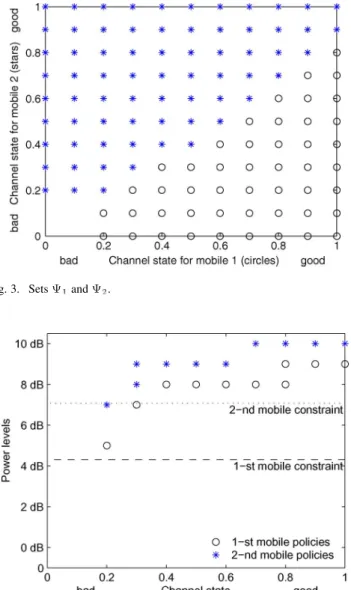
Fig. 3. Sets9 and 9 .
Fig. 4. Supports of the optimal policies in cooperative case.
Once the occupation measures are obtained, the strategies can be computed by means of (2).
Define the following sets:
• : pairs : such that and
for some ;
• : pairs : such that and
for some .
Note, that the set is the set of states in which th player should transmit with nonzero probability according to the op-timal strategy.
In Fig. 3 these sets are provided for the centralized optimiza-tion problem (22). The set is depicted by circles, and the set —by stars. One can see, that the sets have no mutual points. It means, that the mobiles never transmit at the same time. We note that the time-sharing property of the optimal policy was also ob-served in [33] in the context of continuous available power levels in wireless sensor networks.
In Fig. 4 one can see the supports of the optimal strategies. A circle on the place means that the first mo-bile should transmit with the power level with nonzero probability in all states .
A star on the place means that the second mobile should transmit with the power level with nonzero probability in all states .
If there are two or more power levels for some par-ticular state , then the player should randomize. In other case (single power level for the state ), the player should always transmit with power level .
One can see that for both players there are states of randomization. We provide here the strategies
for these states
As one can see, the number of randomizations in the obtained policy exceeds the number of constraints . Nevertheless, due to Theorem 1 the optimal policy can be chosen with no more then randomization points. It is easy to check, that the policy with the same sets and (Fig. 3), supports depicted on Fig. 5, and one randomization point (see the following table) delivers the same value to the cost function:
Note, that the centralized power management provides better throughput in comparison with other considered controls, the value of the cost function is .
Another interesting point that we want to discuss is the attain-ability of the power constraints.
Consider the problem (22) without power constraints. The optimal policies for this problem are as follows:
• Player 1 should transmit at the top power level if ;
• Player 2 should transmit at the top power level if .
The value of the objective function for this policy is
. The experiments show, that at the optimal point for problem with constraints (23), where the bounds are both
Fig. 5. Supports of the optimal policies in cooperative case (one randomization point).
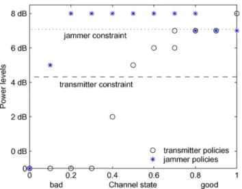
Fig. 6. Supports of the optimal policies in case of jamming.
greater then 7 dB, the power constraints are not attained, and the optimal strategy and the value of the objective function are the same as in unconstrained case.
C. Jamming
The average power bounds are the same as in all previous examples: for the transmitter , and for the jammer
.
The supports of the optimal strategies in this problem are de-picted in Fig. 6. We note that the structure obtained in Theorem 5 holds for player 1, whereas the structure obtained in Section VI holds for player 2. Both players have optimal strategies that are randomized only at one point
The value of the objective function is
which is less then the same value for the decentralized non-co-operative case.
VIII. CONCLUSION ANDFURTHERWORK
We have studied power control in both cooperative and non-cooperative setting. Both centralized and decentralized informa-tion patterns have been considered. We have derived the struc-ture of optimal decentralized policies of selfish mobiles having discrete power levels. We further studied the structure of power control policies when a malicious mobile tries to jam the com-munication of another mobile. We have illustrated these results via several numerical examples, which also allowed us to get insight into the structure in the cooperative framework.
The modeling and results open many exciting research prob-lems. Our setting, which could be viewed as a temporal sched-uling problem, is quite similar to the “space schedsched-uling” (i.e., the water-filling) problems discussed in the introduction, for which the context of discrete power levels along with the nonco-operative setting have not yet been explored. It is interesting not only to study the water-filling problem in the discrete noncoop-erative context but also to study the combined space and tem-poral scheduling problem, where we can split the transmission power both in time and in space (different parallel channels).
From both a game theoretic point of view as well as from the wireless engineering point of view, it is interesting to study pos-sibilities for coordination between mobiles in the decentralized case (in both cooperative as well as non-cooperative contexts). This can be done using the concepts from correlated equilibria [34]–[37], which is known to allow for better performance even in the selfish noncooperative cases. We note however, that ex-isting literature on correlated equilibria do not include side con-straints, which makes the investigation novel also in terms of fundamentals of game theory.
APPENDIX
LINEAR COMPLEMENTARITY APPROACH FOR THEDECENTRALIZEDCASE
In this section we show how the non-cooperative equilib-rium can be obtained in the case of two players by means of linear complementarity problem (LCP). Consider the fol-lowing problem, where each player wants to maximize his own payoff : (24) where ,2 and (25) (26) (27) (28)
Here : is the occupation measure for player ,2.
First, assume, that at the equilibrium point the power con-sumption constraints (28) are active:
(29)
This assumption is not restrictive, because if one or both of these constraints are not active, they can be omitted.
Indeed, let be the policy for player that transmits at all states with maximum power. Then the following statements are easily seen to be equivalent (since the constraints of a player do not depend of the strategies of the other players):
1) at equilibrium, the power constraint of player is met with strict inequality;
2) when using , the power constraint of player is met with strict inequality (independently of the policy of other players).
Any of the statements imply that at equilibrium, is the equi-librium policy of user . So we can first check for which player , the constraints are violated when using policy . For these players, the constraints can be replaced with equality constraints and for the rest, the power constraints can be omitted.
Now let be the vector, containing all the , , , and —the same vector for .
Indeed, the problem (24) with constraints (25)–(27) and (29) can be represented in the form of the bimatrix game with linear constraints (30) s.t. (31) and (32) Following [38] we introduce the linear complementarity problem whose solution characterizes the equilibrium point of (30)–(32):
(33) where
It is also shown in [38], that under the conditions
and Lemke’s algorithm [39] computes a solution of the LCP (33).
It should be noted, that in order to satisfy the conditions , we can always replace cost matrices and with
and , where is a matrix of unities, and is the maximal positive entry of and .
Once the solution of LCP (33) is found, the equilib-rium point of the bimatrix game (30) could be computed using the following formulas:
(34) where and are vectors of appropriate dimension, whose components are all ones.
REFERENCES
[1] W. R. Heinzelman, A. Chandrakasan, and H. Balakrishnan, “Energy-efficient communication protocol for wireless microsensor networks,” in Proc. 33rd Annu. Hawaii Int. Conf. Syst. Sci., Jan. 2000, vol. 8, p. 8020.
[2] C. R. Lin and M. Gerla, “Adaptive clustering for mobile wireless net-works,” IEEE J. Select. Areas Commun., vol. 15, no. 7, pp. 1265–1275, Sep. 1997.
[3] T. J. Kwon and M. Gerla, “Clustering with power control,” in Proc.
IEEE Military Commun. Conf. (MILCOM’99), Atlantic City, NJ, 1999,
vol. 2, pp. 1424–1428.
[4] W. Heinzelman, A. Chandrakasan, and H. Balakrishnan, “An applica-tion-specific protocol architecture for wireless microsensor networks,”
IEEE Trans. Wireless Commun., vol. 1, no. 4, pp. 660–670, Oct. 2002.
[5] A. Mainwaring, D. Culler, J. Polastre, R. Szewczyk, and J. Anderson, “Wireless sensor networks for habitat monitoring,” in Proc. 1st ACM
Int. Workshop Wireless Sensor Networks Appl. (WSNA’02), New York,
NY, 2002, pp. 88–97.
[6] H. Ren and M. Meng, “A game theoretic model of distributed power control for body sensor networks to reduce bioeffects,” in Proc. 3rd
IEEE/EMBS Int. Summer School Medical Devices Biosensors, Sep.
2006, pp. 90–93.
[7] H. Ji and C.-Y. Huang, “Non-cooperative uplink power control in cel-lular radio systems,” Wireless Networks, vol. 4, no. 4, pp. 233–240, Jun. 1998.
[8] R. D. Yates, “A framework for uplink power control in cellular radio systems,” IEEE J. Select. Areas Commun., vol. 13, no. 9, pp. 1341–1347, Sep. 1995.
[9] T. Alpcan, T. Bas¸ar, R. Srikant, and E. Altman, “CDMA uplink power control as a noncooperative game,” Wireless Networks, vol. 8, pp. 659–670, 2002.
[10] D. Falomari, N. Mandayam, and D. Goodman, “A new framework for power control in wireless data networks: Games utility and pricing,” in
Proc. Allerton Conf. Commun., Control Comput., Champaign, IL, Sep.
1998, pp. 546–555.
[11] M. Huang, R. P. Malhamé, and P. E. Caines, “On a class of large-scale cost-coupled Markov games with applications to decentralized power control,” in Proc. IEEE Conf. Decision Control (CDC’04), Atlantis, Paradise Island, Bahamas, Dec. 2004.
[12] L. Lai and H. El Gamal, “The Water-Filling Game in Fading Mul-tiple Access Channels,” IEEE Trans. Inform. Theory, vol. 54, no. 5, pp. 2110–2122, May 2008.
[13] F. Meshkati, M. Chiang, V. Poor, and S. C. Schwartz, “A game-the-oretic approach to energy-efficient power control in multi-carrier CDMA systems,” IEEE J. Select. Areas Commun., vol. 24, no. 6, pp. 1115–1129, Jun. 2006.
[14] D. P. Palomar, J. M. Cioffi, and M. A. Lagunas, “Uniform power allo-cation in MIMO channels: A game-theoretic approach,” IEEE Trans.
Inform. Theory, vol. 49, no. 7, pp. 1707–1727, Jul. 2003.
[15] C. U. Saraydar, N. B. Mandayam, and D. Goodman, “Efficient power control via pricing in wireless data networks,” IEEE Trans. Commun., vol. 50, no. 2, pp. 291–303, Feb. 2002.
[16] C. W. Sung and W. S. Wong, “Mathematical aspects of the power control problem in mobile communication systems,” in Lectures at
the Morningside Center of Mathematics, L. Guo and S. S.-T. Yau,
Eds. Cambridge, MA: ACM/International Press, 2000.
[17] C. Wu and D. P. Bertsekas, “Distributed power control algorithms for wireless networks,” IEEE Trans. Veh. Technol., vol. 50, no. 2, pp. 504–514, Mar. 2001.
[18] S.-L. Kim, Z. Rosberg, and J. Zander, “Combined power control and transmission rate selection in cellular networks,” in Proc. IEEE Veh.
[19] S. G. Glisic, Advance Wireless Communications: 4G Technologies. New York: Wiley, 2004.
[20] O. Popescu and C. Rose, “Water filling may not good neighbors make,” in Proc. IEEE Global Telecommun. Conf. (GLOBECOM’03), San Francisco, CA, Dec. 2003, pp. 1766–1770.
[21] J. B. Rosen, “Existence and uniqueness of equilibrium points for con-cave N-person games,” Econometrica, vol. 33, no. 3, pp. 520–534, Jul. 1965.
[22] E. Altman, Constrained Markov Decision Processes. London, U.K.: Chapman and Hall/CRC, 1999.
[23] E. Altman, O. Pourtallier, A. Haurie, and F. Moresino, “Approximating Nash equilibria in nonzero-sum games,” Int. Game Theory Rev., vol. 2, no. 2–3, pp. 155–172, 2000.
[24] M. Tidball, A. Lombardi, O. Pourtallier, and E. Altman, “Continuity of optimal values and solutions for control of Markov chains with con-straints,” SIAM J. Control Optim., vol. 38, no. 4, pp. 1204–1222, 2000. [25] D. M. Topkis, Supermodularity and Complementarity. Princeton, NJ:
Princeton Univ. Press, 1998.
[26] B. Bencsath, I. Vajda, and L. Buttyán, “A game based analysis of the client puzzle approach to defend against DoS attacks,” in Proc. IEEE
Conf. Software, Telecommun. Comput. Networks (SoftCOM’03), Split,
Croatia, Oct. 2003, pp. 763–767.
[27] P. Kyasanur and N. H. Vaidya, “Detection and handling of MAC layer misbehavior in wireless networks,” in Proc. Int. Conf. Dependable Syst.
Networks (DSN’03), San Francisco, CA, Jun. 2003, pp. 173–182.
[28] M. Kodialam and T. V. Lakshman, “Detecting network intrusions via sampling: A game theoretic approach,” in Proc. IEEE INFOCOM, Mar. 30–Apr. 3 2003, vol. 3, pp. 1880–1889.
[29] E. Altman, K. Avrachenkov, R. Marquez, and G. Miller, “Zero-sum constrained stochastic games with independent state processes,” Math.
Methods Oper. Res. (ZOR), vol. 62, no. 3, pp. 375–386, 2005.
[30] J. B. Lasserre, “Global optimization with polynomials and the problem of moments,” SIAM J. Optim., vol. 11, no. 3, pp. 796–817, 2001. [31] J. B. Lasserre, “Semidefinite programming vs. LP relaxations for
poly-nomial programming,” Math. Oper. Res., vol. 27, no. 2, pp. 347–360, May 2002.
[32] R. Cottle, J.-S. Pang, and R. E. Stone, The Linear Complementarity
Problem. Boston, MA: Academic Press, 1992.
[33] I. C. Paschalidis, W. Lai, and D. Starobinski, “Asymptotically optimal transmission policies for large-scale low-power wireless sensor net-works,” IEEE/ACM Trans. Netw., vol. 15, no. 1, pp. 105–118, Feb. 2007.
[34] R. J. Aumann, “Subjective and correlation in randomized strategies,”
J. Math. Econ., vol. 1, pp. 67–96, 1974.
[35] R. J. Aumann, “Correlated Equilibrium as an expression of Bayesian rationality,” Econometrica, vol. 55, pp. 1–18, 1987.
[36] S. Hart and D. Schmeidler, “Existence of correlated equilibria,” Math.
Oper. Res., vol. 14, pp. 18–25, 1989.
[37] A. Neyman, “Correlated equilibrium and potential games,” Int. J. Game
Theory, vol. 26, pp. 223–227, 1997.
[38] D. Koller, N. Megiddo, and B. von Stengel, “Efficient computation of equilibria for extensive two-person games,” Games Econ. Beh., vol. 14, pp. 247–259, 1996.
[39] C. E. Lemke, “Bimatrix Equilibrium points and Mathematical Pro-gramming,” Manag. Sci., vol. 11, no. 7, pp. 681–689, May 1965.
Eitan Altman (M’93–SM’00) received the B.Sc.
degree in electrical engineering, the B.A. degree in physics and the Ph.D. degree in electrical engi-neering from the Technion-Israel Institute, Haifa, in 1984 and 1990, respectively, and the B.Mus. degree in music composition from Tel-Aviv university, Tel-Aviv, Israel, in 1990.
Since 1990, he has been with National research in-stitute in informatics and control (INRIA), Sophia-Antipolis, France. His current research interests in-clude performance evaluation and control of telecom-munication networks and in particular congestion control, wireless communi-cations and networking games.
Dr. Altman has been the (co)Chairman of the Program Committee of several international conferences and workshops (on game theory, networking games, and mobile networks).
Konstantin Avrachenkov received the M.S.
de-gree in control theory from St. Petersburg State Polytechnic University, St. Petersburg, Russia, in 1996 and the Ph.D. degree in mathematics from the University of South Australia, Adelaide, in 2000.
Currently, he is a Researcher at INRIA Sophia Antipolis, France. His main research interests are Markov chains, Markov decision processes, singular perturbation theory, mathematical programming, and the performance evaluation of data networks.
Ishai Menache received the Ph.D. degree in
elec-trical engineering from the Technion, Haifa, Israel, in 2008.
From 1997 to 2000, he was an Engineer in the Net-work Communications Group, Intel. He is currently a Postdoctoral Associate in the Laboratory for Infor-mation and Decision Systems, Massachusetts Insti-tute of Technology, Cambridge. His research inter-ests include Quality of Service (QoS) architectures in communication networks, and game theoretic anal-ysis of networks, with emphasis on wireless systems.
Gregory Miller was born in Krasnogorsk, Russia,
on November 23, 1980. He received the M.S. and Ph.D. degrees in physics and mathematics from the Moscow Aviation Institute, Moscow, Russia, in 2003 and 2006, respectively, and the Ph.D. degree in infor-matics from the University of Nice, Nice, France, in 2006.
Since 2002, he was been with the Institute of Infor-matics Problems, Russian Academy of Sciences (IPI RAN) as a Research Fellow. His current research in-terests include minimax filtering and control, hidden Markov models and applications in telecommunications.
Balakrishna J. Prabhu (S’99–M’05) received
the M.Sc. degree in electrical communications engineering from the Indian Institute of Science, Bangalore, in 2002 and the Ph.D. degree from the University of Nice-Sophia Antipolis, France, in 2005.
He is currently a CNRS Researcher at LAAS, Toulouse, France. His research interests include per-formance evaluation of communication networks, in particular congestion control, peer-to-peer networks, and wireless networks.
Adam Shwartz (M’86–SM’89) received the B.Sc.
degree in physics and the B.Sc. degree in electrical engineering from Ben Gurion University, Beersheba, Israel in 1979, the M.A. degree in applied mathe-matics and the Ph.D. degree in engineering from Brown University, Providence, RI, in 1982 and 1983, respectively.
Since 1984, he is with the Technion-Israel In-stitute of Technology, where he is Professor of Electrical Engineering and holds The Julius M. and Bernice Naiman Chair in Engineering. He held visiting positions at the ISR—University of Maryland, Mathematical Research center—Bell Labs, Rutgers Business School, CNRS—Montreal, Free Univer-sity Amsterdam and shorter visiting positions elsewhere. His research interests include probabilistic models—in particular the theory of Markov decision processes, stochastic games, and asymptotic methods including diffusion limits and the theory of large deviations—and their applications to computer communications networks.