HAL Id: hal-00317903
https://hal.archives-ouvertes.fr/hal-00317903
Submitted on 14 Oct 2005
HAL is a multi-disciplinary open access
archive for the deposit and dissemination of
sci-entific research documents, whether they are
pub-lished or not. The documents may come from
teaching and research institutions in France or
abroad, or from public or private research centers.
L’archive ouverte pluridisciplinaire HAL, est
destinée au dépôt et à la diffusion de documents
scientifiques de niveau recherche, publiés ou non,
émanant des établissements d’enseignement et de
recherche français ou étrangers, des laboratoires
publics ou privés.
Comparisons between EUV/IMAGE observations and
numerical simulations of the plasmapause formation
V. Pierrard, J. Cabrera
To cite this version:
V. Pierrard, J. Cabrera. Comparisons between EUV/IMAGE observations and numerical simulations
of the plasmapause formation. Annales Geophysicae, European Geosciences Union, 2005, 23 (7),
pp.2635-2646. �hal-00317903�
Annales Geophysicae, 23, 2635–2646, 2005 SRef-ID: 1432-0576/ag/2005-23-2635 © European Geosciences Union 2005
Annales
Geophysicae
Comparisons between EUV/IMAGE observations and numerical
simulations of the plasmapause formation
V. Pierrard1and J. Cabrera2
1Belgian Institute for Space Aeronomy, Brussels, Belgium
2Center for Space Radiations, UCL, 1348 Louvain-La-Neuve, Belgium
Received: 8 March 2005 – Revised: 6 July 2005 – Accepted: 3 August 2005 – Published: 14 October 2005
Abstract. Simulations of plasmapause formation described
in Pierrard and Lemaire (2004) predict the shape and equa-torial distance of the plasmapause as a function of the geo-magnetic activity index Kp. The equatorial positions
pre-dicted by this model are compared with the observations of EUV/IMAGE during the geomagnetic storm of 24 May 2000, substorm events of 10 June 2001 and 25 June 2000, and also during a prolonged quiet period (2 May 2001) when the plasmasphere was very extended. The formation of struc-tures, like plumes and shoulders observed during periods of high geomagnetic activity, is quite well reproduced by the simulations. These structures are directly related to specific time sequences of Kpvariations. The radial distances of the
plasmapause are also reproduced, on average, by the model.
Keywords. Magnetospheric physics (Plasmasphere; Storms
and substorms; Solar wind magnetosphere interactions)
1 Introduction
The plasmasphere constitutes the extension of the ionosphere at high altitude: cold plasma from the ionosphere moves along magnetic field lines and populates flux tubes forming the plasmasphere. The outer surface in the plasmasphere is often characterized by a sharp decrease in the plasma den-sity, called the plasmapause. Whistlers and in-situ satellite observations have revealed that the equatorial position of the plasmapause varies from 2.5 REto 7 REand depends, on
av-erage, on the level of geomagnetic activity (Carpenter and Anderson, 1992; Moldwin et al., 2002).
The first global comprehensive images of the Earth’s plas-masphere were provided by the EUV (Extreme UltraVio-let) instrument on board the IMAGE spacecraft launched in March 2000 (Burch et al., 2001). With these images, the large-scale dynamics of the plasmasphere was revealed. Ir-regular structures at the plasmapause, like shoulders, plumes Correspondence to: V. Pierrard
and channels were identified and analyzed (Sandel et al., 2003).
These new observations give an exceptional opportunity to check the mechanisms proposed for the formation of the plasmapause. It is well admitted that the configuration of cold plasma in the plasmasphere depends on the electric field. This electric field is formed by the interplay of the co-rotation electric field, which dominates near Earth, and the convec-tion electric field, generated by the interacconvec-tion of the solar wind with the magnetosphere. When the geomagnetic ac-tivity level increases, the convection electric field increases and the region where co-rotation is enforced shrinks. The outer streamlines are then depleted. On the contrary, when the convection electric field diminishes, the co-rotation re-gion expands to include some depleted flux tubes, which can then refill by evaporation from the ionosphere and by other possible mechanisms.
In the first theoretical formulation of the plasmasphere, the plasmapause coincided to the last closed equipotential of the electric field after prolonged periods of constant Kp values.
Unfortunately, the magnetospheric electric field is never sta-tionary long enough for such an ideal plasmapause frontier to form. On the contrary, all observations since 1963 indi-cate that the formation of a sharp plasmapause occurs dur-ing magnetic substorm events, when the magnetosphere be-comes suddenly disturbed.
Another mechanism to explain the plasmapause forma-tion has been proposed (Lemaire, 1974; 1985; 2000): the cold plasma distribution becomes convectively unstable in the outermost region of the plasmasphere when the convec-tion electric field is suddenly enhanced. The centrifugal force drives the plasma upwards and then produces a sharp density gradient along the magnetic field lines tangent to the surface where the parallel force is zero (Zero Parallel Force Surface: ZPFS). This mechanism is described in detail in Lemaire and Gringauz (1998). According to this mechanism, the plasma-pause is determined by a convective instability in the post-midnight sector, where the convection velocity is maximum. After an increase in the level of magnetic activity, i.e. an
2636 V. Pierrard and J. Cabrera: Plasmapause formation increase in the Kpvalue, a new plasmapause is formed closer
to the Earth than the last closed equipotential of the electric field.
When Kpincreases, the plasmasphere is peeled off in the
post-midnight LT sector. Due to the depletion of the outer flux tubes, the plasmapause is closer to the Earth in this LT sector. A few hours later, a plume is often generated in the afternoon LT sector due to differential rotation. When Kp
decreases, the ZPFS shifts to larger radial distances. The outer flux tubes beyond the innermost vestigial plasmapause refill until a level of saturation is achieved. If the decrease in Kp is abrupt, a shoulder like those observed by EUV can
develop.
Other explanations have been proposed for the formation of plumes (Grebowsky, 1970) and shoulders (Goldstein et al., 2002). They are based on variations of the convection elec-tric field with parameters and boundary conditions appropri-ately adjusted. By such adjustments, these authors were able to fit the results of their models with a number of observed plasmapause positions.
The simulations presented in the present paper use a given Kp-dependent magnetospheric electric field model without
any adjustment. This electric field is the E5D model deter-mined from dynamical proton and electron spectra measured on board the geostationary satellites ATS-5 and 6 (McIlwain, 1986). The empirical electric field E5D is fully determined by the value of Kp. These simulations developed at IASB
(Pierrard and Lemaire, 2004) are based on the mechanism of instability for the plasmapause formation and thus depend on the values of Kp.
The results of the simulations based on the E5D electric field have been compared with CLUSTER data (Dandouras et al., 2004). The fit between predictions of this model and the CLUSTER observations was quite satisfactory. In the present paper, we compare the prediction of this same model with the global EUV/IMAGE observations of the plasma-sphere. The chosen case studies correspond to substorm events, magnetic storms and prolonged quiet periods.
2 Methodology
The physical mechanisms and the numerical method on which the following simulations are based, are explained, re-spectively, in Lemaire and Gringauz (1998) and Pierrard and Lemaire (2004). The Kp index during the period of time is
the only input of the time-dependent model. Kp determines
uniquely the E5D convection electric field distribution. The post-midnight sector is the region where the convection elec-tric field intensity is the largest and where the plasmapause peeling off is expected to take place according to this model. The plasmapause is formed at the equatorial distance of the deepest penetration of the ZPFS: this is located around 02:00 LT for the E5D model. At subsequent LT, the plasma-pause position is determined by the earlier values of Kp,
re-sulting from the changing electric field distribution and the (E×B)/B2drift motion of the plasmapause.
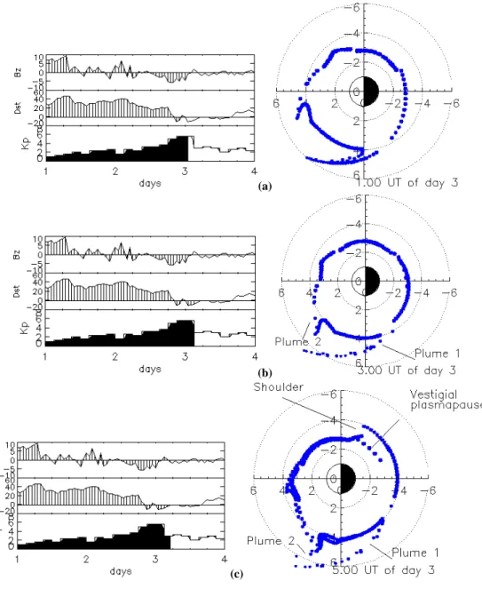
The model predictions are compared with EUV observa-tions from IMAGE. These observaobserva-tions are intensity maps of the 30.4 nm emissions of Helium ions integrated along the line of sight. They are projected in the geomagnetic equa-torial plane in the SM reference system with the program XForm (ftp://euv.lpl.arizona.edu/pub/bavaro/unsupported/), in order to have the same view over the pole as in the sim-ulations. The plasmapause is assumed to be the sharp edge where the brightness of 30.4 nm He+emissions drops dras-tically. To better visualize the plasmapause, we draw a red line corresponding to 40% of the maximum intensity of the image, where the intensity is the logarithm of the luminosity.
3 During a magnetic substorm
Periods of time following an increase in Kp or a magnetic
substorm event are particularly interesting to study because they generally show the development of a so-called plume in the plasmasphere. This kind of plume is often observed in IMAGE observations and follows even moderate increases of Kp(above 3+−4).
3.1 9–10 June 2001
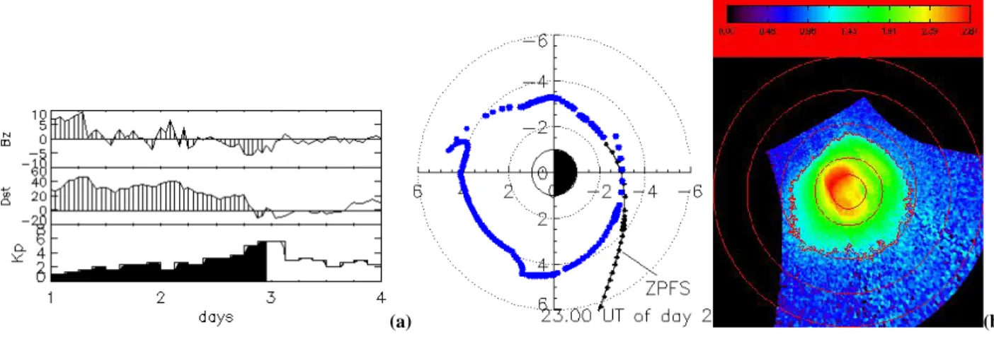
Let us show the example of 9–10 June 2001, for which EUV observations were presented by Spasojevic et al. (2003). The upper panel of Fig. 1a shows Bz, the z component of the
interplanetary magnetic field, the Dst index and the
geomag-netic activity index Kp, observed from 8 June to 10 June
2001. During this period of 3 days, Kp gradually increases
up to 5+and then decreases. Note that during this geomag-netic substorm, the interplanetary maggeomag-netic field turns south-ward during more than 5 h.
The lower panel of Fig. 1a shows the result of the simula-tion on 9 June 2001 at 08:00 UT. Kpis then observed to be
equal to 2+. Due to the rather low value of Kp, the model
predicts a plasmapause quite far from the Earth, around 4 RE.
Because Kp was low and almost constant during the
previ-ous 24 h, the plasmapause is quasi-circular. The circles on the figure correspond to a radial distance of 1, 2, 4 and 6.
The result of the simulation is compared with the plasma-sphere observed by EUV on 9 June 2001 at 08:00 UT, illus-trated in Fig. 1b. The plasmasphere is viewed from a point of view about the North Pole and projected in the geomag-netic equatorial plane. The circles on the figure correspond to a radial distance of 1, 2, 4, 6 and 8 Earth radii. One can see that the plasmapause is indeed quite circular and located near R=4 RE.
Figure 2a illustrates the plasmapause obtained at 16:00 UT, thus 8 h later. Kp has slightly increased, so that
the plasmasphere is eroded in the post-midnight sector above the ZPFS, due to plasma instability. The ZPF surface, illus-trated by the black line in the post-dusk MLT sector, cor-responds to the equatorial cross section, where the effective gravitational acceleration has a zero component parallel to the dipolar magnetic field lines. This surface crosses the
V. Pierrard and J. Cabrera: Plasmapause formation 2637
Figure 1:
Left panel (a): result of the simulation based on the instability mechanism, the E5D
model and the value of Kp on 9 June 2001, 8h00. The plasmapause in the geomagnetic
equatorial plane corresponds to the blue line. The indexes Bz, Dst and Kp observed
during the previous and following days are also displayed. The dotted circles correspond
to L=1, 2, 4 and 6.
Right panel (b): EUV observations on 9 June 2001 at 8h05, projected in the geomagnetic
equatorial plane. The red line corresponds to 40% of the maximum intensity of the image
and permits to visualize the plasmapause. The red circles correspond to L=1, 2, 4, 6 and
8.
a
b
18
(a)Figure 1:
Left panel (a): result of the simulation based on the instability mechanism, the E5D
model and the value of Kp on 9 June 2001, 8h00. The plasmapause in the geomagnetic
equatorial plane corresponds to the blue line. The indexes Bz, Dst and Kp observed
during the previous and following days are also displayed. The dotted circles correspond
to L=1, 2, 4 and 6.
Right panel (b): EUV observations on 9 June 2001 at 8h05, projected in the geomagnetic
equatorial plane. The red line corresponds to 40% of the maximum intensity of the image
and permits to visualize the plasmapause. The red circles correspond to L=1, 2, 4, 6 and
8.
a
b
18
(b)
Fig. 1. (a) Result of the simulation based on the instability mechanism, the E5D model and the value of Kpon 9 June 2001, 08:00. The
plasmapause in the geomagnetic equatorial plane corresponds to the blue line. The indexes Bz, Dst and Kp, observed during the previous
and following days, are also displayed. The dotted circles correspond to L=1, 2, 4 and 6. (b) EUV observations on 9 June 2001 at 08:00 UT, projected in the geomagnetic equatorial plane. The red line corresponds to 40% of the maximum intensity of the image and permits one to visualize the plasmapause. The red circles correspond to L=1, 2, 4, 6 and 8.
Fig. 2: Same as Fig. 1 for 9 June 2001, 16h00 (left panel (a), simulation) and 16h04 UT
(right panel (b), EUV observation). The black line on the left panel corresponds to the
Zero Parallel Force Surface.
a
b
Fig. 3: Same as Fig. 1 for 9 June 2001, 23h00 (left panel (a), simulation) and 23h04 UT
(right panel (b), EUV observation).
a
b
(a)
Fig. 2: Same as Fig. 1 for 9 June 2001, 16h00 (left panel (a), simulation) and 16h04 UT
(right panel (b), EUV observation). The black line on the left panel corresponds to the
Zero Parallel Force Surface.
a
b
Fig. 3: Same as Fig. 1 for 9 June 2001, 23h00 (left panel (a), simulation) and 23h04 UT
(right panel (b), EUV observation).
a
b
19
(b)
Fig. 2. Same as Fig. 1 for 9 June 2001, 16:00 UT ((a), simulation) and 16:04 UT ((b), EUV observation). The black line on the left panel
corresponds to the Zero Parallel Force Surface.
plasmasphere only in the post-midnight sector and only when Kp increases. This is why the plasmasphere is peeled off in
this sector during geomagnetic substorms in the simulations. On Fig. 2b, one can see that the plasmasphere observed by IMAGE at 16:04 is indeed eroded in the post-midnight sector and that the plasmapause is formed closer to the Earth in this sector.
Figure 3a illustrates the plasmapause obtained at 23:00 UT (7 h later), when Kp becomes maximum (5+). Again, the
plasmasphere is peeled off in the post-midnight region due the increase in convection velocity, above the ZPFS illus-trated by the black curve. Since the plasmasphere has ro-tated, the plasmapause is also close to the Earth in the
morn-ing sector. Small structures that will form the plumes begin to appear at the plasmapause in the simulation. The EUV IM-AGE observation in Fig. 3b confirms that the plasmapause forms indeed closer to the Earth in the post-midnight re-gion. But there are substantial differences between the two figures. Whereas the minimum radial expansion is at 02:00– 03:00 LT in the model, it is at 07:00–08:00 LT in the IM-AGE view. The small bump obtained in the simulation in the pre-noon sector is not observed by IMAGE. This bump is, in fact, due to the peeling off process considered in the simula-tion. Combined with the differential rotation, it leads to the development later on of a plume that becomes well visible in the afternoon sector in Figs. 4 a, b and c, corresponding,
2638 V. Pierrard and J. Cabrera: Plasmapause formation
Fig. 2: Same as Fig. 1 for 9 June 2001, 16h00 (left panel (a), simulation) and 16h04 UT
(right panel (b), EUV observation). The black line on the left panel corresponds to the
Zero Parallel Force Surface.
a
b
Fig. 3: Same as Fig. 1 for 9 June 2001, 23h00 (left panel (a), simulation) and 23h04 UT
(right panel (b), EUV observation).
a
b
19
(a)Fig. 2: Same as Fig. 1 for 9 June 2001, 16h00 (left panel (a), simulation) and 16h04 UT
(right panel (b), EUV observation). The black line on the left panel corresponds to the
Zero Parallel Force Surface.
a
b
Fig. 3: Same as Fig. 1 for 9 June 2001, 23h00 (left panel (a), simulation) and 23h04 UT
(right panel (b), EUV observation).
a
b
19
(b)Fig. 3. Same as Fig. 1 for 9 June 2001, 23:00 ((a), simulation) and 23:04 UT ((b), EUV observation).
respectively, to 10 June 2001 at 01:00, 03:00, and 05:00 UT. The plumes in the simulations are shown by the blue dots that extend to large radial distances. The dots correspond to plasma elements located at the plasmapause.
Two different plumes (referred as “Plume 1” and “Plume 2”) developed in the afternoon and dusk sector during this pe-riod of time. In the simulations, plumes develop after plas-maspheric erosion due to differential rotation, i.e. because the plasma convects more slowly around the Earth at large radial distance than closer to the Earth. Several plumes can sometimes develop during a period of time, corresponding to a Kp increase. Such a plasmasphere with two different
plumes has sometimes been observed by EUV.
Moreover, the sudden decrease in Kp at 03:00 UT leads
to the formation of a shoulder in the dawn sector, as seen on Fig. 4c. Indeed, when Kpdecreases, the plasmapause should
extend further away from the Earth, since the ZPFS has then shifted to larger radial distances. Since the refilling process of the flux tubes is slower than the peeling off process and can sometimes take several days, we also draw the “vestigial plasmapause”, which is then closer to the Earth in the dawn LT sector and appears after a Kpdecrease.
Unfortunately, it is not possible to compare the results of the simulation presented in Fig. 4 with EUV observations, since the IMAGE satellite is too close to the Earth to provide any global view of the plasmasphere during this period of time. The EUV observations are regularly interrupted along the orbit of the satellite, so that it is not easy to follow con-tinuously the formation of plumes and their evolution with time. The observations have generally a typical duration of 7 h (with a time resolution of 10 min) out of each 14-h or-bit. Just after an interruption, the satellite is still far from its apogee, so that the observations are not of very good quality, as is the observation on 10 June 2001 at 05:00 UT and this is why it is not shown in the present paper. But it is interesting to note that Plume 2 and the shoulder are already present at that time in the observations. The external edge of the plume is quite irregular at that time, so that Plume 1 can be roughly distinguished.
In Fig. 5a, we show the results of the simulation on 10 June 2001 at 07:00 UT. Plume 1 has become so thin that it has almost disappeared. The blue dots visible in the dusk and midnight sectors are the remains of this Plume 1. Plume 2 is well visible in the dusk LT sector. The shoulder has rotated.
Figure 5b shows the EUV/IMAGE observation at 07:00 UT. Plume 2 is indeed observed in the same LT sec-tor as predicted by our simulations. The presence of a thin Plume 1 is not clear, but not excluded. The shoulder is clearly shown by the observations, but there is a slight delay in MLT compared to the model prediction, as if Kp had in fact
de-creased earlier than in the measurements. Note that Kp is
a three-hour index, and leads to a ±03:00 UT or ±3 MLT indetermination.
The presence of a well-structured shoulder at that time suggests another mechanism than the slow refilling of the plasma flux tubes, since the evaporation process from the ionosphere is generally quite inefficient in night-dawn LT sectors. As a complementary mechanism, interchange can also contribute to the shoulder formation: dips and blobs, trapped below the new ZPFS, rearrange so that the mate-rial internal to the new plasmapause boundary contributes to the shoulder shaped feature of the outer plasmasphere. Small-scale plasma density structures were indeed observed by CLUSTER mainly in the dusk sector during or after ge-omagnetic substorms (Darrouzet et al., 2004). These small-scale density structures, explained with the plasma instabil-ity theory (Lemaire, 1974), are not clearly seen at the same time in the corresponding EUV images, since the EUV in-strument cannot resolve spatial structures with a size smaller than 0.1 RE (Darrouzet at al., 2004). Moreover, small-scale
density structures are difficult to detect by EUV, due to the line of sight integration and to the average lower threshold of the EUV corresponding to 40 electrons/cm3(Goldstein et al., 2004).
A few detached plasma elements were observed in situ in the post-midnight sector by Chappell et al. (1971), but at least some of these large-scale structures can correspond to co-rotating plumes. More recently, the EUV scanner on board
V. Pierrard and J. Cabrera: Plasmapause formation 2639
Fig.4: Simulation of the development of plumes on June 10, 2001 at 1h00 (left panel (a)),
3h00 (right panel (b)) and 5h00 (bottom panel (c)). IMAGE is too close to the Earth to
provide a global view of the plasmasphere during this period of time.
a
b
c
20
(a)
Fig.4: Simulation of the development of plumes on June 10, 2001 at 1h00 (left panel (a)),
3h00 (right panel (b)) and 5h00 (bottom panel (c)). IMAGE is too close to the Earth to
provide a global view of the plasmasphere during this period of time.
a
b
c
20
Fig.4: Simulation of the development of plumes on June 10, 2001 at 1h00 (left panel (a)),
3h00 (right panel (b)) and 5h00 (bottom panel (c)). IMAGE is too close to the Earth to
provide a global view of the plasmasphere during this period of time.
a
b
c
20
(b)
Fig.4: Simulation of the development of plumes on June 10, 2001 at 1h00 (left panel (a)),
3h00 (right panel (b)) and 5h00 (bottom panel (c)). IMAGE is too close to the Earth to
provide a global view of the plasmasphere during this period of time.
a
b
c
20
Fig.4: Simulation of the development of plumes on June 10, 2001 at 1h00 (left panel (a)),
3h00 (right panel (b)) and 5h00 (bottom panel (c)). IMAGE is too close to the Earth to
provide a global view of the plasmasphere during this period of time.
a
b
c
20
(c)Fig.4: Simulation of the development of plumes on June 10, 2001 at 1h00 (left panel (a)),
3h00 (right panel (b)) and 5h00 (bottom panel (c)). IMAGE is too close to the Earth to
provide a global view of the plasmasphere during this period of time.
a
b
c
20
Fig. 4. Simulation of the development of plumes on 10 June 2001 at 01:00 UT (a), 03:00 UT (b) and 05:00 UT (c). IMAGE is too close tothe Earth to provide a global view of the plasmasphere during this period of time.
Planet-B revealed that there is a significant amount of plas-maspheric ions escaping from the duskside outer plasmas-phere toward the magnetosplasmas-phere (Yoshikawa et al., 2000).
Note that the shoulder could also be due to an expansion of the plasmaspheric plasma up to the new plasmapause after the sharp decrease in Kp. In this case, the number density of
the particles inside the inner plasmasphere should be slightly lower than before the formation of the shoulder. The EUV observations of Figs. 6b and 7b show that the shoulder con-tinues to expand outwards even after 07:00 UT. More studies cases would be useful to determine the mechanisms involved in the formation of shoulders.
Later on, Kp remains almost constant and small (<2+).
The simulation shows how the plume and the shoulder
ro-tate with the Earth and evolve. This can be seen in Figs. 6a and 7a, corresponding, respectively, to 10 June 2001, 10:00 and 12:00 UT. EUV observations at 09:57 UT in Fig. 6b and 12:00 in Fig. 7b show that the shoulder moves slowly out-ward. The clearly identifiable plume becomes thinner with time. The rotation seems quite slower in the dusk than in other LT sectors, so that the plume wraps and becomes cap-tured. This process creates a density depletion that is mostly extended in azimuth, as shown in Fig. 7b.
In all EUV figures corresponding to the present case study, we use the threshold 0.40 of the maximum intensity to draw the limit of the plasmasphere. A lower threshold would give a red line a little bit further from the Earth, where the thin plasma depletion shown in Fig. 7b is less indented. The
2640 V. Pierrard and J. Cabrera: Plasmapause formation
Fig. 5: Same as Fig. 1 for 10 June 2001, 7h00 (left panel (a), simulation) and 7h03 UT
(right panel (b), EUV observation).
a
b
b
Fig. 6: Same as Fig. 1 for June 10, 2001, 10h00 (left panel (a), simulation) and 9h57 UT
(right panel (b), EUV observation).
a
b
21
(a)Fig. 5: Same as Fig. 1 for 10 June 2001, 7h00 (left panel (a), simulation) and 7h03 UT
(right panel (b), EUV observation).
a
b
b
Fig. 6: Same as Fig. 1 for June 10, 2001, 10h00 (left panel (a), simulation) and 9h57 UT
(right panel (b), EUV observation).
a
b
21
(b)Fig. 5. Same as Fig. 1 for 10 June 2001, 07:00 UT ((a), simulation) and 07:00 UT ((b), EUV observation).
Fig. 5: Same as Fig. 1 for 10 June 2001, 7h00 (left panel (a), simulation) and 7h03 UT
(right panel (b), EUV observation).
a
b
b
Fig. 6: Same as Fig. 1 for June 10, 2001, 10h00 (left panel (a), simulation) and 9h57 UT
(right panel (b), EUV observation).
a
b
21
(a)
Fig. 5: Same as Fig. 1 for 10 June 2001, 7h00 (left panel (a), simulation) and 7h03 UT
(right panel (b), EUV observation).
a
b
b
Fig. 6: Same as Fig. 1 for June 10, 2001, 10h00 (left panel (a), simulation) and 9h57 UT
(right panel (b), EUV observation).
a
b
21
(b)
Fig. 6. Same as Fig. 1 for 10 June 2001, 10:00 ((a), simulation) and 09:57 UT ((b), EUV observation).
relative intensity threshold procedure provides slightly dif-ferent plasmapause positions than those obtained by the man-ual procedure used by Spasojevic et al. (2003) to determine the plasmapause position.
Note that there is no free parameter (i.e. no ad hoc fetch fitting parameter) used in our simulations to improve the fit with observations. Only the observed values of Kpare used
as input with McIlwain’s E5D and M2 electric and magnetic field models. Of course, it could be possible to improve the results of such model simulations by adding or adjust-ing some parameters, but the goal of the present study is not to obtain the “best fit” with the observations. The goal is to check whether the formation of the plasmapause by an inter-change mechanism does approximately reproduce the overall feature and evolution of the plasmapause observed with the EUV instrument.
3.2 25 June 2000
Another example of plume formation was observed between 25 and 26 June 2000. Figure 8a shows the result of our sim-ulation obtained at 21:00 UT on 25 June. The plasmapause is rather extended, due to the low values of Kp in the
pre-vious hours. The plasmasphere is also quite circular due to the stationarity of Kp during the previous 24 h. The quiet
period was, however, preceded by a substorm the day before, that is why the vestigial plasmapause is also shown closer to the Earth at R=3.8 RE in the afternoon sector. The vestigial
plasmapause corresponds to the inner points. Above this ves-tigial plasmapause, the outer flux tubes of the plasmasphere are supposed to refill up to the external plasmapause.
The EUV observations in Fig. 8b show the quasi-circular plasmasphere at 21:03 on 25 June. The observed plasma-pause is quite close to the Earth and suggests that the outer flux tubes are not yet fully refilled. Note, nevertheless, that
V. Pierrard and J. Cabrera: Plasmapause formation 2641
Fig. 7: Same as Fig. 1 for June 10, 2001, 12h00 (left panel (a), simulation) and 12h00 UT
(right panel (b), EUV observation).
a
b
Fig. 8: Same as Fig. 1 for June 25, 2000, 21h00 (left panel (a), simulation) and 21h03 UT
(right panel (b), EUV observation).
a
b
22
(a)Fig. 7: Same as Fig. 1 for June 10, 2001, 12h00 (left panel (a), simulation) and 12h00 UT
(right panel (b), EUV observation).
a
b
Fig. 8: Same as Fig. 1 for June 25, 2000, 21h00 (left panel (a), simulation) and 21h03 UT
(right panel (b), EUV observation).
a
b
22
Fig. 7: Same as Fig. 1 for June 10, 2001, 12h00 (left panel (a), simulation) and 12h00 UT
(right panel (b), EUV observation).
a
b
Fig. 8: Same as Fig. 1 for June 25, 2000, 21h00 (left panel (a), simulation) and 21h03 UT
(right panel (b), EUV observation).
a
b
22
(b)
Fig. 7. Same as Fig. 1 for 10 June 2001, 12:00 ((a), simulation) and 12:00 UT ((b), EUV observation).
Fig. 7: Same as Fig. 1 for June 10, 2001, 12h00 (left panel (a), simulation) and 12h00 UT
(right panel (b), EUV observation).
a
b
Fig. 8: Same as Fig. 1 for June 25, 2000, 21h00 (left panel (a), simulation) and 21h03 UT
(right panel (b), EUV observation).
a
b
22
(a)
Fig. 7: Same as Fig. 1 for June 10, 2001, 12h00 (left panel (a), simulation) and 12h00 UT
(right panel (b), EUV observation).
a
b
Fig. 8: Same as Fig. 1 for June 25, 2000, 21h00 (left panel (a), simulation) and 21h03 UT
(right panel (b), EUV observation).
a
b
22
(b)
Fig. 8. Same as Fig. 1 for 25 June 2000, 21:00 UT ((a), simulation) and 21:03 UT ((b), EUV observation).
the satellite is located quite close to the Earth at that time, so that the global view of the plasmasphere is restricted.
In the dawn sector, one can see a density depletion that is mostly extended in the radial direction (a “channel”). These kinds of features were discovered in the EUV observations and permit one to measure the rotation velocity of the plas-masphere at different radial distances, which is often lower than co-rotation (Spasojevic et al., 2003). The observed channel can be due to a plume wrapping, as illustrated in the previous case of 10 June 2001, but other origins may be possible.
On 26 June 2000, Kp increases up to 6 during a
geomag-netic substorm and this leads to the formation of a plume in our simulations. We show the development of the plume obtained in the simulation in Figs. 9a and b, at 03:00 and 09:00 UT. The formation of the plume begins in the pre-noon sector in the simulation, but it is only well formed and iden-tifiable as a plume when it reaches the afternoon sector.
Un-fortunately, EUV doesn’t provide any observation during this period since the satellite IMAGE is too close to the Earth to give a global view of the plasmasphere.
In Fig. 10a, the result of the model is shown on 26 June 2000 at 16:00 UT. A nice plume has developed due to the Kpincrease and is now well structured. This plume is clearly
seen in the same LT sector in the EUV image corresponding to the same time, shown in Fig. 10b. The position of the plasmapause is observed to be slightly closer to the Earth than in the simulation. The plasmapause density gradients are very sharp, as is often the case after such events, and the plasmapause position is well defined in the integrated inten-sity plots of EUV.
We have analyzed over ten of such events where Kp
in-creases. Although the results do not fit exactly the obser-vations, our simulations reproduce rather satisfactorily the erosion of the plasmasphere followed by the formation of plumes during geomagnetic substorms. Plumes are always
2642 V. Pierrard and J. Cabrera: Plasmapause formation
Fig. 9: Simulation of the development of the plume on June 26, 2000 at 3h00 (left panel
(a)) and 9h00 (right panel (b)). IMAGE could not give global views of the plasmasphere
during this period of time.
a
b
Fig. 10: Same as Fig. 1 for June 26, 2000, 16h00 (left panel (a), simulation) and 15h56
UT (right panel (b), EUV observation).
a
b
23
(a)
Fig. 9: Simulation of the development of the plume on June 26, 2000 at 3h00 (left panel
(a)) and 9h00 (right panel (b)). IMAGE could not give global views of the plasmasphere
during this period of time.
a
b
Fig. 10: Same as Fig. 1 for June 26, 2000, 16h00 (left panel (a), simulation) and 15h56
UT (right panel (b), EUV observation).
a
b
23
(b)
Fig. 9: Simulation of the development of the plume on June 26, 2000 at 3h00 (left panel
(a)) and 9h00 (right panel (b)). IMAGE could not give global views of the plasmasphere
during this period of time.
a
b
Fig. 10: Same as Fig. 1 for June 26, 2000, 16h00 (left panel (a), simulation) and 15h56
UT (right panel (b), EUV observation).
a
b
23
Fig. 9. Simulation of the development of the plume on 26 June 2000 at 03:00 UT (a) and 09:00 UT (b). IMAGE could not give global views
of the plasmasphere during this period of time.
Fig. 9: Simulation of the development of the plume on June 26, 2000 at 3h00 (left panel
(a)) and 9h00 (right panel (b)). IMAGE could not give global views of the plasmasphere
during this period of time.
a
b
Fig. 10: Same as Fig. 1 for June 26, 2000, 16h00 (left panel (a), simulation) and 15h56
UT (right panel (b), EUV observation).
a
b
23
(a)Fig. 9: Simulation of the development of the plume on June 26, 2000 at 3h00 (left panel
(a)) and 9h00 (right panel (b)). IMAGE could not give global views of the plasmasphere
during this period of time.
a
b
Fig. 10: Same as Fig. 1 for June 26, 2000, 16h00 (left panel (a), simulation) and 15h56
UT (right panel (b), EUV observation).
a
b
23
(b)
Fig. 10. Same as Fig. 1 for 26 June 2000, 16:00 UT ((a), simulation) and 15:56 UT ((b), EUV observation).
formed in the afternoon LT sector a few hours after an in-crease in Kp. Subsequently, the plumes slowly rotate when
the geomagnetic activity decreases.
4 During a geomagnetic storm: 24 May 2000
During magnetic storms, Dst decreases during a main phase
and then recovers over about one day. Kpincreases then
usu-ally up to high values ranging between 7 and 9. For instance, on 24 May 2000, Kp increased up to 8 (see Fig. 11a, upper
panel) and Dstdrops to −130 nT. Although the origin of
V. Pierrard and J. Cabrera: Plasmapause formation
Fig. 11: Same as Fig. 1 for May 24, 2000, 9h00 (left panel (a), simulation) and 9h02 UT
2643(right panel (b), EUV observation). A plume develops in the afternoon sector in the
simulation as in the observations.
a
b
Fig. 12: Same as Fig. 1 for May 2, 2001, 18h00 (left panel (a), simulation) and 17h58 UT
(right panel (b), EUV observation).
a
b
24
(a)
Fig. 11: Same as Fig. 1 for May 24, 2000, 9h00 (left panel (a), simulation) and 9h02 UT
(right panel (b), EUV observation). A plume develops in the afternoon sector in the
simulation as in the observations.
a
b
Fig. 12: Same as Fig. 1 for May 2, 2001, 18h00 (left panel (a), simulation) and 17h58 UT
(right panel (b), EUV observation).
a
b
24
(b)Fig. 11. Same as Fig. 1 for 24 May 2000, 09:00 ((a), simulation) and 09:02 UT ((b), EUV observation). A plume develops in the afternoon
sector in the simulation as in the observations.
Fig. 11: Same as Fig. 1 for May 24, 2000, 9h00 (left panel (a), simulation) and 9h02 UT
(right panel (b), EUV observation). A plume develops in the afternoon sector in the
simulation as in the observations.
a
b
Fig. 12: Same as Fig. 1 for May 2, 2001, 18h00 (left panel (a), simulation) and 17h58 UT
(right panel (b), EUV observation).
a
b
24
(a)
Fig. 11: Same as Fig. 1 for May 24, 2000, 9h00 (left panel (a), simulation) and 9h02 UT
(right panel (b), EUV observation). A plume develops in the afternoon sector in the
simulation as in the observations.
a
b
Fig. 12: Same as Fig. 1 for May 2, 2001, 18h00 (left panel (a), simulation) and 17h58 UT
(right panel (b), EUV observation).
a
b
24
(b)
Fig. 12. Same as Fig. 1 for 2 May 2001, 18:00 ((a), simulation) and 17:58 UT ((b), EUV observation).
of the large increase in Kpalso has the effect to peel off the
plasmasphere in the post-midnight region and to develop a well-defined plume.
Figure 11a shows the result of the simulation at 09:00 UT. A plume is formed due to the increase in Kpand a shoulder
due to the sharp decrease in Kp. Since the increase in Kpis
large, the plasma elements corresponding to the blue dots on Fig. 11a are spaced when the plume is formed. The plasma-pause corresponds to an imaginary line joining these dots. The presence of two different boundaries in afternoon LT sector (one near Earth; one at higher radial distance) means that the plume which formed in the afternoon sector is, in fact, quite thin.
This figure can be compared with the observations, pre-sented in Fig. 11b and also prepre-sented by Burch et al. (2001). The plume is well visible in the same LT sector. A shoulder is also present, although not so distinctly as in our simulations.
The radial distance of the plasmapause corresponds on aver-age, to what is obtained in the simulation. It is only slightly closer to the Earth than during geomagnetic substorms.
5 During a very quiet period: 2 May 2001
When Kp is very low during a long period of time, the
plasmapause is located far from the Earth, since the flux tubes have been refilling for enough time to approach sat-uration. An example of a very quiet and extended period is presented in Fig. 12a by the result of the simulation at 18:30 UT on 2 May 2001, when Kpremained lower than 2−
for over 2 days. The EUV observations at 18:28 UT are illus-trated in Fig. 12b: the plasmasphere is very extended and the gradients in density are very smooth over the whole field of view. There does not appear to be a sharp knee in the plasma density profiles. Thus, the plasmapause position, as drawn
2644 V. Pierrard and J. Cabrera: Plasmapause formation
Fig. 13: Radial distance of the plasmapause observed at 3h00 MLT in the EUV observations for all 4 periods of time presented in this paper. When the Kp index decreases, symbols are red diamonds (◊); they are black crosses (+) when Kp increases. The blue stars represent the plasmapause position found with the instability model for a constant value of Kp. The pink line corresponds to the linear relation found by Moldwin et al. (2002) between L and Kp for average plasmapause crossings observed by CRRES in the dawn LT sector between August 1990 and October 1991.
25 Fig. 13. Radial distance of the plasmapause observed at 03:00 MLT
in the EUV observations for all 4 periods of time presented in this paper. When the Kpindex decreases, symbols are red diamonds ♦;
they are black crosses (+) when Kpincreases. The blue stars
repre-sent the plasmapause position found with the instability model for a constant value of Kp. The pink line corresponds to the linear
rela-tion found by Moldwin et al. (2002) between L and Kpfor average
plasmapause crossings observed by CRRES in the dawn LT sector between August 1990 and October 1991.
by the red line, is very dependent on the adopted threshold value. In this figure, like in the other figures in this paper, the threshold is 40% of the maximum intensity.
Whistler and satellite observations have also shown that after a quiet period of time, the density gradients are gener-ally very smooth. On the contrary, the plasmapause is very sharp after a peeling-off event, when the level of geomag-netic activity increases abruptly!
6 Radial distance of the plasmapause
It is also interesting to perform a statistical study of the radial distance of the plasmapause observed by EUV in the post-midnight sector, where the plasmapause is formed with the mechanism of plasma instability. The plasmapause positions at 03:00 LT are displayed in Fig. 13 as a function of Kp.
The crosses and diamonds represent the radial distance of the plasmapause observed by EUV at 03:00 LT for the 4 periods of time considered in this paper.
Red diamonds are used when the Kpindex decreases
(fol-lowing a geomagnetic storm or substorm); black crosses are used when Kpincreases (following a quiet period). There is
a significant scatter among the experimental results, indicat-ing that the plasmapause also depends on other parameters than Kp, but it is quite clear that the plasmapause position
is located closer to the Earth when Kp is large. This
con-firms many earlier whistler and spacecraft observations. The pink straight line in Fig. 13 corresponds to the linear rela-tion found by Moldwin et al. (2002) between L and Kp for
CRRES data in the dawn LT sector.
This figure also shows that the plasmapause is closer to the Earth when Kp decreases (diamonds) than when Kp
increases (crosses), which indicates that the peeling-off ef-fect takes place when geomagnetic activity is enhancing, and that during the following period of quieting, the plasmapause tends to expand radially outward. As a result of this follow-up radial expansion, the plasma density inside the plasma-sphere is expected to be reduced, as indeed observed since many years through the whistler technique (Carpenter and Lemaire, 1997). The blue stars represent the theoretical plasmapause position predicted by the instability model in case Kpwould have been independent of time.
7 Conclusions and discussion
The following results are obtained from the direct compar-ison between the EUV observations from IMAGE and nu-merical simulations of the plasmapause position determined from the value of Kp using the instability mechanism with
the E5D electric field model:
1. Plumes are produced by our simulations after a moder-ate increase in Kp. They develop in the afternoon
sec-tor. The base of the plume rotates faster than its top during the quieting period following the enhanced mag-netic activity, so that the plume is deformed and wraps in the dusk sector. Plumes are indeed observed by EUV during geomagnetic storms in the same LT sectors; 2. Observed shoulders are produced just at the end of
mag-netic substorms or storms; they generally develop one or two hours before a sharp decrease in Kp;
3. Very steep gradients of density are observed in the post-midnight sector, where the peeling-off effect is the most important, according to the instability scenario and the McIlwain E-field empirical model;
4. For a given value of Kp, the EUV data show that the
plasmapause positions are rather widely scattered about an average value. The plasmapause position is not sim-ply determined by the instantaneous Kp value, but it
also depends on its past history, i.e. if it was increasing or decreasing before the current time. On average, the plasmapause position is a nonlinear function of Kp,
al-though a clear linear trend is found for large values of Kp;
5. The instability theory for the formation of the plasma-pause qualitatively accounts for a range of dynamical plasmaspheric events and observed features;
6. The results of our simulations could be improved by introducing other effects or by adjusting some param-eters in the simulations. For instance, in the present simulations, we use the empirical model of E5D that includes the co-rotation velocity and the convection ve-locity. Nevertheless, some studies have revealed that
V. Pierrard and J. Cabrera: Plasmapause formation 2645 in the range 2<L<4, the plasma frequently rotates at a
rate of 85–90% of the co-rotation (Sandel et al., 2003). The simulations adapted with a lower rotation velocity sometimes give a better agreement with the EUV obser-vations. A plasmaspheric wind in the radial direction can also have some effects.
We present here some typical cases of comparisons be-tween our simulations of the plasmapause formation and EUV observations. Other cases also show a rather good agreement. But of course, these results do not mean that all features observed with EUV can be simulated in detail with the numerical code. Moreover, these results do not exclude that tails and shoulders can also be formed by other proposed mechanisms. The role of the sub-auroral polarization stream (SAPS) in the plume formation and in the sunward transport of plasma from dusk is, for instance, more and more empha-sized in the recent literature (Foster and Vo, 2002; Goldstein et al., 2003; Spasojevic et al., 2004).
It is also clear that the quasi-static E5D electric field model has inherent limitations and is certainly not the ultimate elec-tric field we need for space weather predictions. E5D has a time resolution limited to 3 h, due to its Kp dependence.
Moreover, Liemohn et al. (2004) noted that E5D is good at predicting the plasmapause location in the post-midnight sec-tor, but it is too weak in the noon sector to account for the EUV observations during the recovery phase of the 17 April 2002 magnetic storm.
Despite these limitations, such comparisons and future ad-ditional ones allow us to identify the similarities and the dis-crepancies between the results of the simulations and the ob-servations. This work helps to improve the theory for the formation of the plasmapause, as well as the empirical mod-els of the inner magnetospheric electric field.
Acknowledgements. The authors thank B. Sandel, Lunar and
Plan-etary Laboratory, University of Arizona, Tucson, USA and D. L. Gallagher, NASA, National Space Science and Technology Center, Huntsville, USA for the access to the EUV observations of the satel-lite IMAGE. The authors thank also J. Lemaire for discussions and commenting the manuscript. V. Pierrard thanks the Belgian PPS for the financial support (grant MO/35/010).
Topical Editor T. Pulkkinen thanks P. D´ecr´eau and another ref-eree for their help in evaluating this paper.
References
Burch, J. L., Mende, S. B., Mitchell, D. G., Moore, T. E., Pollock, C. J., Reinisch, B. W., Sandel, B. R., Fuselier, S. A., Gallagher, D. L., Green J. L., Perez, J. D., and Reiff, P. H.: Views of Earth’s Magnetosphere with the IMAGE Satellite, Science, 291, 619– 624, 2001.
Carpenter, D. L. and Anderson, R. R.: An ISEE/whistler model of equatorial electron density in the magnetosphere, J. Geophys. Res., 97(A2), 1097–1108, 1992.
Carpenter, D. L. and Lemaire, J.: Erosion and recovery of the plas-masphere in the plasmapause region, Space Sci. Rev., 80, 153– 179, 1997.
Chappell, C. R., Harris, K. K., and Sharp, G. W.: The dayside of the plasmasphere, J. Geophys. Res., 76, 7632–7647, 1971. Dandouras, I., Pierrard, V., Goldstein, J., Vallat, C., Parks, G. K.,
R`eme, H., Gouillart, C., Sevestre, F., McCarthy, M., Kistler, L. M., Klecker, B., Korth, A., Bavassano-Cattaneo, M. B., Es-coubet, Ph., and Masson, A.: Multipoint observations of ionic structures in the Plasmasphere by CLUSTER-CIS and compar-isons with IMAGE-EUV observations and with Model Simula-tions, accepted for publication in Yosemite 2004 AGU Mono-graph, 2004.
Darrouzet, F., D´ecr´eau, P. M. E., De Keyser, J., Masson, A., Gal-lagher, D. L., Santolik, O., Sandel, B. R., Trotignon, J. G., Rauch, J. L., Le Guirriec, E., Canu, P., Sedgemore, F., Andr´e, M., and Lemaire, J. F.: Density structures inside the plasmasphere: Clus-ter observations, Ann. Geophys., 22, 2577–2585, 2004,
SRef-ID: 1432-0576/ag/2004-22-2577.
Foster, J. C. and H. B. Vo: Average characteristics and activity de-pendence of the subauroral polarization stream, J. Geophys. Res., 107(A12), 1475, doi:10.1029/2002JA009409, 2002.
Goldstein, J., Sandel, B. R., Hairston, M. R., and Reiff, P. H.: Control of plasmaspheric dynamics by both convection and sub-auroral polarization stream, J. Geophys. Res., 30(24), 2243, doi:10.1029/2003GL018390, 2003.
Goldstein, J., Spiro, R. W., and Reiff, P. H., et al.: IMF-driven overshielding electric field and the origin of the plasmaspheric shoulder of 24 May 2000, Geophys. Res. Lett., 16, 66–1:4, doi:10.1029/2001GL014534, 2002.
Goldstein, J., Sandel, B. R., Thomsen M. F., Spasojevic, M., and Reiff, P. H.: Simultaneous remote sensing and in situ obser-vations of plasmaspheric drainage plumes, J. Geophys. Res., 109(A03202), doi:10.1029/2003JA010281, 2004.
Grebowsky, J. M.: Model study of plasmapause motion, J. Geo-phys. Res., 75, 4329–4333, 1970.
Lemaire, J.: The “Roche limit” of ionospheric plasma and the for-mation of the plasmapause, Planet. Space Sci., 22, 757–766, 1974.
Lemaire, J. F.: Frontiers of the plasmasphere (Theoretical aspects), Universit´e Catholique de Louvain, Facult´e des Sciences, Editions Cabay, Louvain-La-Neuve, ISBN-2-87077-310-2, 1985. Lemaire, J. F.: The formation plasmaspheric tails, Phys. Chem.
Earth (C), 25, 1–2, 9, 2000.
Lemaire J. F. and Gringauz, K. I.: With contributions from Car-penter, D. L. and Bassolo, V. (Ed.): The Earth’s plasmasphere, Cambridge University Press, Cambridge, 1998.
Liemohn M. W., Ridley, A. J., Gallagher, D. L., Ober, D. M., and Kozyra J. U.: Dependence of plasmaspheric morphology on the electric field description during the recovery phase of the 17 April 2002 magnetic storm, J. Geophys. Res., 109(A03209), doi:10.1029/2003JA010304, 2004.
McIlwain, C. E.: A Kp dependent equatorial electric field model,
The Physics of Thermal plasma in the magnetosphere, Adv. in Space Res., 6 (3), 187–197, 1986.
Moldwin, M. B., Downward, L., Rassoul, H. K., Amin, R., and An-derson, R. R.: A new model of the location of the plasmapause: CRRES results, J. Geophys. Res., 107, 1339:1–9, 2002. Nishida, A.: Formation of plasmapause, or magnetsopheric plasma
knee, by the combined action of magnetospheric convection and plasma escape from the tail, J. Geophys. Res., 71, 5669–5679, 1966.
Pierrard V. and Lemaire, J.: Development of shoulders and plumes in the frame of the interchange instability mechanism for plasmapause formation, Geophys. Res. Lett., 31, 5(L05809),
2646 V. Pierrard and J. Cabrera: Plasmapause formation doi:10.1029/2003GL018919, 2004.
Sandel B. R., Goldstein, J., Gallagher, D. L., and Spasojevic, M.: Extreme ultraviolet imager observations of the structure and dy-namics of the plasmasphere, Space Sci. Rev., 109, 25–46, 2003. Spasojevic, M., Goldstein, J., Carpenter, D. L., Inan, U. S.,
Mold-win, M. B., and Reinisch, B. W.: Global response of the plas-masphere to a geomagnetic disturbance, J. Geophys. Res., 108, 1340, doi:10.1029/2003JA009987, 2003.
Spasojevic M., Frey, H. U., Thomsen, M. F., Fuselier, S. A., Gary, S. P., Sandel, B. R., and Inan, U. S.: The link between a detached subauroral proton arc and a plasmaspheric plume, Geophys. Res. Lett., 31(L04803), doi:10.1029/2003GL018389, 2004.
Yoshikawa, I., Yamazaki, A., Shiomi, K., Yamashita, K., Takizawa, Y., and Nakamura, M.: Evolution of the outer plasmasphere during low geomagnetic activity observed by the EUV scanner onboard Planet-B, J. Geophys. Res., 105(A12), 27 777–22 789, 2000.