Long-term variation of the temperature of the middle atmosphere at mid-latitude: dynamical and radiative causes

HAL Id: insu-03123430

https://hal-insu.archives-ouvertes.fr/insu-03123430

Submitted on 28 Jan 2021

HAL is a multi-disciplinary open access

archive for the deposit and dissemination of

sci-entific research documents, whether they are

pub-lished or not. The documents may come from

teaching and research institutions in France or

abroad, or from public or private research centers.

L’archive ouverte pluridisciplinaire HAL, est

destinée au dépôt et à la diffusion de documents

scientifiques de niveau recherche, publiés ou non,

émanant des établissements d’enseignement et de

recherche français ou étrangers, des laboratoires

publics ou privés.

Long-term variation of the temperature of the middle

atmosphere at mid-latitude: dynamical and radiative

causes

Marie-Lise Chanin, N. Smirès, Alain Hauchecorne

To cite this version:

Marie-Lise Chanin, N. Smirès, Alain Hauchecorne.

Long-term variation of the temperature

of the middle atmosphere at mid-latitude: dynamical and radiative causes.

Journal of

Geo-physical Research: Atmospheres, American GeoGeo-physical Union, 1987, 92 (D9), pp.10933-10941.

�10.1029/JD092iD09p10933�. �insu-03123430�

JOURNAL OF GEOPHYSICAL RESEARCH, VOL. 92, NO. D9, PAGES 10,933-10,941, SEPTEMBER 20, 1987

LONG-TERM VARIATION OF THE TEMPERATURE OF THE MIDDLE ATMOSPHERE AT MID-LATITUDE' DYNAMICAL AND RADIATIVE CAUSES

M. L. Chanin, N. Smirks, and A. Hauchecorne

Service d'A•ronomie, Centre National de la Recherche Scientifique,

Verri•res-le-Buisson, France

Abstract. Temperature of the middle they have been observed in stratospheric ozone atmosphere has been measured since 1979 at the [Keating et al., 1981] and temperature [Angell

Observatory of Haute-Provence (France, 44øN, 6øE) and Korshover, 1978' Quiroz, 1979]. Furthermore,

using the Rayleigh lidar technique. More than 500 the few observations of solar-related variations

temperature profiles in the height range 35-75 km not only disagree with the models, but they are have been used in that study. The main results far from agreement with each other' they differ are the following' temperature trends of opposite not only in the amplitude of the effect but also

sign have been observed in the mesosphere (-20øK in its sign.

at 65 km) and in the stratosphere (+20øK at The altitude range concerned in this paper

40 km) between 1981 and 1985' but while the trend includes both the upper stratosphere and the

in the stratosphere is only found in winter, the mesosphere. This region has been traditionally tendency in the mesosphere is observed all year studied by rocket techniques, from which most of around. These temperature changes exhibit a the published data have been obtained. Satellite highly significant correlation with the solar data in the stratosphere suffer from possible flux (represented by the radio flux at 10.7 cm) instrument drift and from a too short lifetime in the mesosphere and an equally significant and have not been used for study of long-term

anticorrelation in the winter stratosphere. On variation.

the other hand, the temperature at the 50-km In this study we present the results of a

level does not present any long-term variation. long-term temperature survey performed at middle

These results are interpreted as due to a latitude using a Rayleigh lidar' this technique

superposition of a direct response of the provides absolute temperature profiles unaffected

mesosphere to the increase of the UV flux and a by any instrumental drift. We first summarize the

second effect, mainly present in winter, which results obtained on temperature trends before

affects all height ranges. This effect may or not

presenting the lidar

data and their

interpreta-

be related

to the 11-year solar cycle, but its

tion. We then show how this

interpretation can

height dependence and its sign can only be explain most of the observations.

interpreted by a change in the planetary wave

activity.

Brief Summary

of Observed

Temperature

Trends

and

Introduction

'Their Relationship With ii-Year Solar Cycle

Most studies of long-term trends of the middle

The attempt to detect any possible trend in

the middle atmosphere

structure and composition atmosphere

temperature

have

been

conducted

having

in mind a possible solar cycle relationship. To

has induced a tremendous effort by both modelists

and experimenters. In order to separate

solar-induced variations (whether they are direct or indirect) from a possible anthropogenic effect

in interpreting the observations, different

models have attempted to evaluate the direct

effect of solar UV variations on the compositeion,

mention first the mesosphere, where the results

are the least confusing, we refer to the more

recent and more extensive study by Mohanakumar

[1985]: the analysis concerns the height range

50-80 km and is based on rocket data from four

stations ranging from 81øN to 69øS: Heyss Island

(81øN, 58øE), Volgograd (49øN, 44øE), Thumba

temperature,

and dynamics

of the stratosphere. (8øN, 77øE), and Molodezhnaya

(69øS,

46øE).

A

The results of these models have been strongly

dependent

upon the assumed

amplitude

of the UV- clear positive correlation is observed

between

flux variability' the earlier ones,

based

in part

number

Rz and the mesospheric

temperature

with a

on the estimates

of Heath

and

Thekaekara

[1977], maximum

amplitude

of about

10øK

around 65-70 km

had a tendency to overestimate the solar

for all seasons.

This result is in general

variability. Only the more recent models, which _{agreement (independently of the number of the}

use a more realistic estimate of the UV flux

solar cycle) with the earlier results of Kokin

et

variation, will be used for reference [Brasseur al. [1981] at 81øN, Von Cossart and Taubenheim

and Simon, 1981' Garcia et al., 1984]. The

[1987] at 49øN,

and

Devanarayanan

and

Mohanakumar

predicted

influence

of the 11-year

cycle on the [1985a] at 8øN But surprisingly,

the data

collected by Devanarayanan and Mohanakumar

few degrees at most around the stratopause.

Models taking into account

the direct uV

[1985b] between

28øN and 34øN, during the

response of the atmosphere

underestimate preceding

solar cycle, did not indicate any

definite correlation in the height range

systematically the amplitude of the variations as _{50-65 km.}

In the stratosphere the situation is more

Copyright 1987 by the American Geophysical Union. complex. Until 1982 all of the authors, with the

exception of Kokin et al. [1981], reported a

Paper number 7D0618. positive response of the stratosphere to the 0148-0227/87/007D-0618505.00 solar activity [Schwentek, 1971; Zlotnik and

10•934 Chanin et al.: Temperature Variation in Middle Atmosphere

Roswoda, 1976; Angell and Korshover, 1978, 1983; and to get rid of most of the short-period

Quiroz, 1979; Schwentek and Elling, 1981]; the gravity waves. Under these conditions the

data were all concerned with solar cycle 19 and absolute accuracy is iøK at 70 km since 1985; in

20. The more extensive study, and the one more the early phase of the measurements, the accuracy

often mentioned, is that of Quiroz [1979] who was always better than IøK at 50 km and below.

used a large set of rocket data from seven sites. The period covered by this paper extends from A first disagreement with these results came with 1979 to 1985 and includes 519 temperature the paper of Kokin et al. [1981], who found a profiles. The temporal coverage depends upon negative response in winter at the altitude of meteorological conditions. in the recent years

45 km above Heyss island• Later, Schwentek and and more specifically since 1982, when the

Elling [1984], analyzing the Berlin radiosonde station started to be operated on a routine

data for the period 1970-1982 (cycle 20-21), did basis, an average of more than 100 nights of data not confirm the results obtained for the period is obtained each year.

1958-1971, and they put into doubt their own

results published earlier. More recently, Analysis of the Lidar Temperature Data

Devananayanan and Mohanakumar [1985a, b] found

opposite results at 8øN and 28ø-34N ø. The In order to separate clearly long-term from confusion observed in the stratosphere from the short-term variability, a study of the day-to-day data obtained by rockets was lately tentatively variability was performed successively for each

explained by the fact that a change occurred in year of data. Unless the gap in the series of

1970 in the corrections applied to the rocket data was too large (>10 days), individual data

data; as a consequence, Watson et al., [1986] were interpolated to provide a set of one profile

recommended that those data should not be used to per day. The variance was calculated at each

infer long-term variations. level for each individual profile as the In the lower stratosphere the radiosonde deviation from the 45-day running mean. The

network has been largely used for detecting results were then smoothed with a Blackman window

climatologic trends. A decrease of temperature of to suppress all variation with periods less than the order of 0.3 ø per decade around 20 km has 20 days, which were mostly due to planetary been found on a global basis [Labitzke et al., waves. The yearly maps of variance were shown to 1986; Oehlert, 1986]. They attributed this have the same characteristics from year to year,

cooling to the increase of CO2, as it

was

therefore justifying

the decision to compile

apparently not related to any solar activity several years to provide a mean seasonal effect. More recently, radiosonde data have been variation of the variance. These data were studied to detect local changes which may be already published up to 1984 as part of the lidar

associated with the Antarctic ozone hole, and contribution to the new CIRA model by Chanin et

large changes of temperature have been found to al. [1985]. The more recent results for the

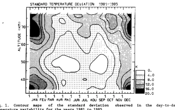
occur locally [Newman and Schoeberl, 1986]. period 1981-1985 are given in Figure 1. Because

of intense planetary wave activity, the winter

Description of the Data Set period corresponds to a much larger variance than

the summer. One also notices a systematic

The experimental data used for this study were difference between the equinoxes, the mesosphere

obtained at the Observatory of Haute-Provence, in autumn being already disturbed with planetary

France (44øN, 6øE) during the period 1979-1985, wave activity. Furthermore, in the winter period

using the Rayleigh lidar technique. The a region of low variability exists around 50 km

measurement technique is based on the between two well-defined maxima situated around

backscattering of a pulsed laser beam by 70-65 and 35-40 km. Those maxima correspond to atmospheric molecules; the temporal analysis of variation of opposite phase associated with the

the echo by time-gating provides the vertical stratospheric warmings and mesospheric coolings.

profile of the atmospheric density. The method is We will come back to that point later in the

described in detail in several publications discussion. But this preliminary study suggests [Hauchecorne and Chanin, 1980; Chanin and that, in order to look for a long-term trend, one Hauchecorne, 1984], and only relevant indications should study separately the data for the will be given here. The downward limit of the different seasons, since, at first thought, the

atmospheric density measurements is imposed by large day-to-day variability in winter could hide

the aerosol upper limit, which is usually 30 km any trend. Thus the data were considered by group

but was raised to 35 km during the E1 Chich6n of 3 months each : December-January-February

posteruption period. The upward limit is given by (DJF) for winter, March-April-May (MAM) for

the sky background level and has been pushed up spring, June-July-August (JJA) for summer, and

from 75 km in 1979 to 95 km since 1985. In order September-October-November (SON) for autumn. The

to use an homogeneous set of data, we chose to reason for separating both equinoxes in the study

limit our study to the height range 35-75 km. was the asymmetry observed in the short-term

The temperature deduced from the density variability.

profile, using the hypothesis of a perfect gas in To get rid of another possible source of

hydrostatic equilibrium, is given in absolute short-term variability, which may come from the value. It does not require any calibration, and solar rotation, we average the data over a month; the data are free of any long-term intrument this method of averaging is more convenient to drift. The data are acquired with good time and use for comparison between successive years than vertical resolutions, which are superfluous when the 27-day average, and we checked to see that it

looking at long-term variation. Time integration did not affect the final results. The behavior of

for the whole period of measurement during the these monthly averaged temperature values as a

same night (-3 hours) and reduction of the height function of time is presented in Figure 2, from

Chanin et al.: Temperature Variation in Middle Atmosphere 10,935

STANDARD TEMPERATURE DEVIATION 1981-:985

I I ',' I ' '1 ' ' I ' ' I ' ' I ' ' I ' ' I ' ' I ' ' I ' ' 'I ' ' I ' ' ' I

Fig. 1. Contour maps of the standard deviation observed in the day-to-day

temperature variability for the years 1981 to 1985.

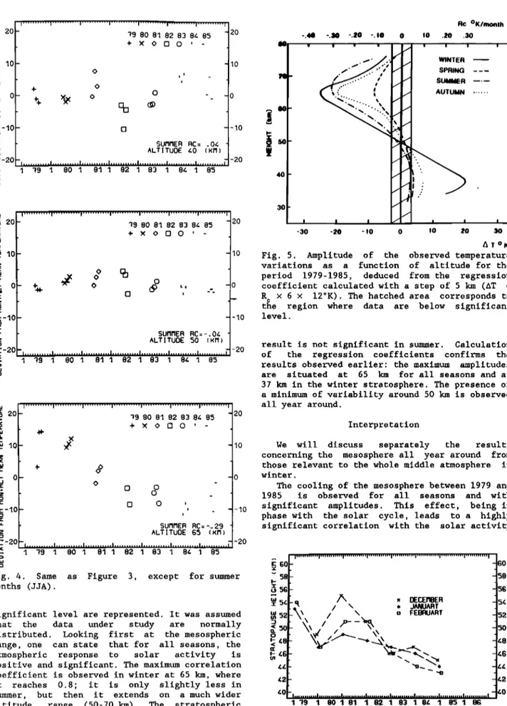
average over 1 year has been calculated and is month is given on each plot of Figures 3 and 4. superimposed on each graph in order to smooth out From this coefficient one can evaluate the the seasonal variation. The monthly mean solar magnitude of the temperature change over the flux at 10.7 cm has been plotted for comparison 6-year period as a function of altitude and on Figure 2, as it will be of use in the season. Those results are presented in Figure 5,

discussion. which summarizes the height distribution and the

Without further analysis several features can seasonal variation of the observed trends.

be readily seen. Two well-defined trends are Several features should be pointed out: in the

visible above and below 50 km, starting around mesosphere, the summer, autumn, and winter

the end of 1981: an increase of 20øK at 40 km and effects are of about the same amplitude, while

a decrease of the same magnitude at 65 km. the amplitude for spring is much smaller.

Independently of the sign, the magnitudes of the Furthermore, the effects for both winter and

observed changes are much larger than predicted autumn are more sharply peaked (at 65 km) than

by models (-IøK). On the other hand, the smoothed for summer and spring, for which the maximum

temperature is observed to be quite stable at extends up to 70 km. In the stratosphere the only

50 km. period for •hich the effect is of the same order

As indicated earlier, the study is performed of magnitude as in the mesosphere is the winter,

separately for each season; furthermore, in order

with a maximum

sharply peaked at 37 km; the

to take into account the seasonal variation of effect in autumn is weaker, while in summer and

the temperature, the quantity which is considered

spring it is barely significant.

is the deviation of each monthly averaged value

The observed opposite variations

in the

from the corresponding monthly mean. This

stratosphere and mesosphere

could induce a change

quantity is plotted as a function of time

in the height of the stratopause. We plotted in

successively for the different altitudes from 35

Figure 6 the average height of the stratopause

to 75 •m, with a step of 5 km, and for each

calculated by fitting

the temperature profiles

season; Figures 3 and 4 show representative

with a parabolic

shape. Even though the

examples

of the different behaviors observed at

scattering of the data is quite large, mainly for

40,

50, and 65 km for winter and summer

the first period 1979-1982, it clearly shows that

conditions. These altitudes are selected because the altitude of the winter stratopause has been

they correspond

to either a maximum

or a minimum going down

during the period 1979-1985.

of variability. The opposite trends in the

mesospheric and stratospheric temperatures are Relationship With Solar Cycle

very well observed in winter; Figure 3 shows

clearly that the changes at both levels only The fact that the changes observed in the

start after the winter of 1981-1982. The absence temperature took place mostly after the start of

of variability at 50 km is confirmed. The the decreasing phase of the solar flux cannot be situation during the summer (Figure 4) is ignored (cf. Figure 2). Even though the data set

slightly different at 65 km, even though the is far too short to establish a solar-induced

decrease of temperature is almost as large as in relationship, we investigate further a winter, but the drop in temperature is already speculative possibility: Figure 2 seems to

visible in 1981. The trends observed at 40 km and indicate that locally the atmosphere is

50 km in summer are below the significant level. responding positively to solar activity in the

The linear regression coefficient (Rc) has mesosphere and negatively in the stratosphere.

10,936 Chanin et al.' Temperature Variation in Middle Atmosphere I ... i ... ! ... i ... i ... I ... i ... 2BO :)4O •0 26O 240 • 20 ,,,, 220

"-' 280

F

• 10

Fig ß 2 . Monthly mean of the temperature measured J

by lidar between 40 and 65 km and monthly mean of z

the 10.7 cm solar flux during the period

•o

1979-1985. A running mean over a year is o

superimposed on each set of data.

• -20

activity which may influence the middle

atmosphere behavior would be the UV flux around

There was no question of limiting our period of observation, which was already quite short; therefore we decided to use the 10.7-cm radio flux, which has been shown to be reasonably well correlated with the solar UV flux, when looking

for long-term variation [London et al., 1984].

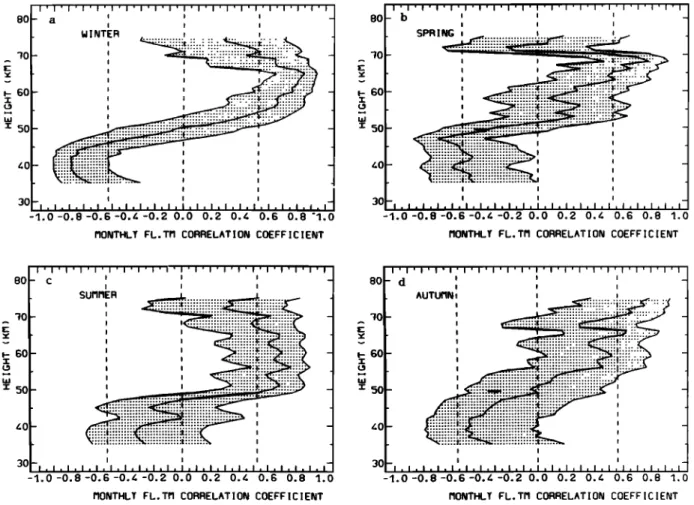
The correlation coefficients have been

calculated for the four seasons and are presented

in Figure 7. The 95% confidence limit and the 99%

1 ... I ... I ... I ... I ... I ... I ... - ':/9 80 81 82 83 84 85 + X 0 r-I 0 ' - - ! o o o WINTER RC: . 25 ALT!TUDE 40 (KFI) , ... , ... , ... ; ... , ... , ... , ... I t9 I 80 I 81 I 82 I 83 I 8/-. I 85 1 - 20 10 0 -10 -20 I ... I ... I ... I ... l ... I ... I ... - t9 80 81 82 83 84 85 20 + X 0 O ' 10 0 0

•

o

_•

_qh

_o

o

_

INTER

Re=

.01

-+

Xx

¾

o

200 nm. At the time when this study was Fig. 3. Temperature deviation from the monthly performed, no such data set was available for the average of the individual monthly mean values for

whole period of 1979 to 1985' the SME data the period 1979-1985, as a function of time. The

started to be available in October 1981. The individual points are given for the three winter

Solar Backscattered Ultraviolet (SBUV) data were months (DJF) of each year at three different only available until 1983 (D.F. Heath, private altitude levels 40, 50, and 65 km. The value of communication ; 1986) and the index based on the the regression coefficient R is given in degrees C

Chanin et al.' Temperature Variation in Middle Atmosphere 10,937 ß 20 '" 10 0 o ,,- -10 o o ,_ -20 uJ ß 20 '" 10 •- 0 ,- -10 o o • -20 1 ... I ... I ... I ... I ... I ... I ... - 79 80 81 82 83 84 85 + X 0 [] 0 ' - 0 i - .4.. 0 0 - . [] SUMMER RC= .04 ALTITUDE 40 (KM) -i ... i ... i ... i ... i ... i ... i ... i I 79 I 80 I 81 I 82 I 83 I 84 I 85 1 -20 10 -0 -10 -20 1 ... I ... I ... I ... I ... ! ... I ... _ 79 80 81 82 83 84 85 + X O [] O ' - 1 Rc øK/monlh -30 -20 -I0 0 I0 20 30 A T OK

-•0 Fig. 5. Amplitude of the observed temperature

variations as a function of altitude for the

O

•

period 1979-1985, deduced

from the regression

- •

O

•)

•,,

-•

0

coefficient

calculated

with a step of 5 km (AT =

t•e region where data are below significant

- -10 level. SUMMER RC:-.04 ALTITUOE 50 (KM) I ... I ... I ... 1 ... I ... I ... I ... , 0 I '39 i 80 I 81 I 82 I 83 I 84 I 85 z _J z o s- z: -10 o z o ,_ -20

result is not significant in summer. Calculation

of the regression coefficients confirms the

results observed earlier: the maximum amplitudes

are situated at 65 km for all seasons and at

37 km in the winter stratosphere. The presence of

a minimum of variability around 50 km is observed

all year around.

n o o [] o Interpretation SUMMER RC:-,.29 ALTITUDE G5 (KM) We wi l 1 discuss •n•r•t•l v th• r•,,] •

concerning the mesosphere all year around from

those relevant to the whole middle atmosphere in

0 winter.

The cooling of the mesosphere between 1979 and 1985 is observed for all seasons and with

significant amplitudes. This effect, being in

phase with the solar cycle, leads to a highly

significant correlation with the solar activity

I,,,,,,,,,,,I ... I ... I ... I ... I ... I ... •,1

I '39 I 80 I 81 1 $2 1 83 1 84 1 85

Fig. 4. Same as Figure 3, except for summer

months (JJA).

-2O

significant level are represented. It was assumed

that the data under study are normally

distributed. Looking first at the mesospheric

range, one can state that for all seasons, the

atmospheric response to solar activity is

positive and significant. The maximum correlation coefficient is observed in winter at 65 km, where

it reaches 0.8; it is only slightly less in

summer, but then it extends on a much wider

altitude range (50-70 km). The stratospheric

behavior is drastically different: whereas the

• 60 - • . o 5(; - '-' ,/• - -,-54 R x DECEMBER ,... / \ o JANUART .

:n

52•-•\ /

\

o FEBRUARI'

g [ '•,• •/..•.•

x

x.

-

negative correlation is very significant in Fig. 6. Mean stratopause height as a function of winter and slightly less during equinoxes, the years for the three winter months.

10,938 Chanin et al.' Temperature Variation in Middle Atmosphere 8O 3O •- 60 T 50 4O 30-- I'l'l'l'l' I 'l'l'l"l'l'-l' I' I'1'!'1'1'1'1'1 I I I - • I i i WINTER , , , • ...::::::•i!iii:'!.:::i!•" I I _ I I _ I•l•l•l,l,l,l,l,l,l,l,l,l,l,l,l,l,l,l,j•l .0-0.8-0.6-0.•-0.2 0.0 0.2 0.• 0.6 0.8 '1.0 MONTHLY FL. TI9 CORRELAT I ON COEFF I C [ENT

8O 30 •- 60 -r 50 40 3O

MONTHLY FL. TI9 CORRELAT I ON COEFF I C I ENT

80 J AUTU•N• 30 - ..:iiii!iiiiiii!i!ii!i'::-

• '

t

::::::::iiiiiiii::'i!!.:::t::iii!i:"

Fig. 7. Correlation coefficient (with _+95% confidence limits) between the monthly mean values of temperature and solar flux at 10.7 cm for (a) winter (DJF)' (b) spring

(M_AM)' (c) summer (JJA)' and (d) autumn (SON). The significant level of 99% is

indicated by the extreme vertical dotted lines.

maximizing around 65-70 km. Such a response of

the mesosphere to variation of the US/ solar flux

is mostly the result of UV absorption by

molecular oxygen around 200 nm and is expected to

decrease with decreasing altitude, as a result of

the smaller variability of the UV flux at the

longer wavelengths which penetrate deeper into

the atmosphere. This is in agreement with the

decrease of the effect from 65 to 50 km, as

observed in Figure 5. The presence of a maximum

of variability around 70 km can be explained by the fact that around that altitude 20% of the

total heating is due to the Lyman • radiation,

whose variability is much larger than in the

200-nm range [Brasseur et al., 1986]. However, if

the sensitivity to solar radiation is observed at

the altitude where it is expected to occur, the

observed amplitudes are much larger than those

calculated by the models.

Furthermore, the response to solar UV should

be the strongest in summer. If the seasonal

variation reflects the variation of the absorbed

UV flux at mid-latitude, then we would expect a

minimum in the winter and intermediate response

during the equinoxes. The amplitude of the summer

effect (ATma

x =-21øK)

is, in fact, observed to

be larger than during spring (ATma X -- -9øK). On

the other hand, both the winter and autumn

effects (ATma

x -- -25øK and -19øK, respectively)

are much larger than expected and do not present

the same height dependance. We interpret the

large values found in winter and autumn as due to

the superposition of two separate effects of

different nature, the weaker effect being the

direct influence of the solar UV variation just

mentioned.

The second effect, mainly observed in winter,

leads to a response of 18øK in the stratosphere

and close to 20øK in the mesosphere (if one

subtracts from the observed value the expected

radiative response of a few degrees K). This

behavior is displayed in Figure 5, with two

maxima of similar amplitude but opposite signs

sharply peaked around 65 km and 35 km, with a minimum at 50 km. This feature is identical to the one we have described in the short-term temperature variability in winter, under the

influence of planetary waves, and displayed in

Figure 1 (even though the opposite sign between

stratospheric and mesospheric temperature

deviation does not appear on this figure, since

the quantity represented is the square root of

the variance). We also noticed in Figure 1 that

the upper mesosphere is quite disturbed in autumn

and this may explain why the long-term behavior

of the temperature in autumn is so similar in

amplitude and height distribution to the winter

one in the mesosphere, while it differs in the

stratosphere.

Chanin et al.' Temperature Variation in Middle Atmosphere 10•939

Chanin, Planetary waves-mean flow interaction in whole solar cycle. It is worth mentioning that in

the middle atmosphere' modelization and comparison this model a strong depletion of O 3 is predicted

with lidar observations, submitted to Annales to occur around 70 km' this decrease in O 3 should

Geophysicae, 1987) that the variability be reflected by a increase in temperature at the

represented in Figure 1 is clearly related to same altitude, which is not present, probably

planetary wave activity and can be understood because of the simplified cooling parametrization

completely in terms of planetary wave propagation. (Newtonian cooling) used in the model. This

So we conclude that the long-term variability discrepancy between observation and models should

observed in wintertime is being induced by be investigated further.

planetary waves. Furthermore, the highly In the stratosphere the radiative effect is so

significant correlation with the solar cycle in small compared to the dynamical ones that the

both the stratosphere and the mesosphere in winter comparison should exclude all the data obtained

may give a strong indication that the atmospheric during winter and even autumn. Then a large part

response to solar flux variation involves an of the discrepancies observed in the experimental

indirect mechanism producing a change in planetary results vanish (except for Zlotnik and Rozwoda

wave activity, only seen in winter when planetary [1976], who report of a 15øK amplitude in summer

waves can propagate upwards in the middle between 1964 and 1971 at 40 km). For the other

atmosphere. authors the amplitudes observed in summer in the

A very important consequence of a long-term

stratosphere are of a few degrees K and, when

change in planetary wave activity, whether or not measurable, they indicate a positive correlation

it is induced by the solar variability,

is that

with the solar activity.

However, most of the

the observed trends will be strongly latitudinal

recent data (Angell

and Korshover [1983]'

dependent and their

local amplitudes may differ

Schwentek

and Elling [1984]' and that reported in

largely from what is observed on a zonal mean.

this paper) indicate that the effect is below the

significant level. This result is not in

Discussion

disagreement

with the models which predict,

at

The results presented

earlier are now compared the maximum,

an amplitude of 2øK at the tropics

with other observations and with model and less than iøK at middle latitudes [Garcia et

expectation. We will

focus the

discussion

al., 1984].

•

successively on the two different causes of

None of

the previously mentioned models

variability' radiation and dynamics.

include a

possible dynamical solar-induced

The direct response

of the atmosphere to UV

mechanism, even though the

influence

of

irradiance variability has been observed to reach

solar-induced dynamics has been proposed and

a maximum

in the mesosphere

around 65-70 km (see

discussed by several authors [Hines, 1974' Bates,

earlier discussion). This result is in agreement

1977' Chandra, 1985, 1986]. In fact,

the models

with

results published earlier

[Mohanakumar, used for prediction

are two-dimensional models

1985' Von Cossart and Taubenheim, 1987], even

which cannot represent

the

planetary

wave

though their results obtained for the whole year

interactions'

anyhow, modelists are

still

have maximum

amplitudes of 12øK and 6øK,

uncertain about what indirect mechanism

has to be

introduced in the models. The mechanism proposed

respectively, compared with our yearly average

value of 18øK. Such a discrepancy in amplitude

by Hines [1974] assumes some change in the

may

be lowered if the data were all treated by

reflection or absorption of planetary waves

under

season' but the important fact is that the maxima solar-disturbed conditions and is expected to be

are localized around the same altitude. It should more relevant to middle and high latitudes in

be noted that the different results obtained in winter. Such a statement is in agreement with our

the two successive

papers of Devahanarayan

and

results. Significant effects in

the middle

Mohanakumar

[1985a, b] can now

be understood, as

atmosphere temperature ozone and winds were

they refer to different altitude ranges,

with the

predicted

by the detailed calculations

of Callis

second one being close to the minimum

of

et al. [1985], but they have not been confirmed

variability.

on long term variation. Observational

evidence

of

Neither the height distribution nor the

solar variability effects on planetary wave

amplitude

of these results have

been

predicted

by

activity have been, until now, limited to the

the models. In a recent paper, Brasscur

et al.

time scale of the solar rotation period. In the

lower stratosphere, Ebel et al. [1986] reported

[1987], presenting the middle atmosphere response

to solar activity, limit the model

calculation to

significant results indicating 27- and 13.5-day

pressure below 0.1 mbar

(-62 km), as the

periods

coherent with the 10.7-cm

flux between

radiative scheme

has not been developed to take

the 50- and 10-mbar levels. The winter results

into account the mesosphere.

Anyhow,

and from

reported in this paper are the first evidence of

simplified calculations, they estimate that the

the long term effect of planetary wave activity

positive correlation of the temperature with

in the upper stratosphere

and mesosphere.

solar activity should

peak around

70 km, with an

This interpretation could explain part of the

amplitude

of 0.25øK

per 1% of solar variation at

confusion

in the already published

results. The

205 nm. This would correspond

to about 2.5øK at

disagreement

mentioned earlier in the sign and

the most if using the extreme values of UV

amplitude of the

results

of

solar-induced

variability

given by SBUV [Lean, 1986]. This

variations of stratospheric temperature may be

amplitude is far below the observed ones and it

understood if a large fraction of this variation

may indicate some

missing heating mechanism in

is linked to the planetary wave activity.

There

the model. The same conclusion can be drawn for is a priori no reason to have a positive response

the Garcia et al. [1984] Rodel' the sensitivity in the mesosphere and a negative one in the

of the temperature to a change in the solar flux stratosphere, as in the case reported here, which

increases with altitude in the mesosphere, but could only be characteristic of a specific site

10,940 Chanin et al.' Temperature Variation in Middle Atmosphere

situation would be occurring elsewhere and/or

scope of this paper and the answer will

require

during other periods. The stratospheric winter analysis of longer series of data.

temperature at Berlin may have exhibited

different causes of variation

during successive

Acknowledgments. The authors are grateful

to

decades, as reported by Schwentek [1971] (-20øK the technical staff of the lidar team for their

at 35 km) and later

in $chwentek and Elling

help in operating the station, in particular,

to

[1984] (<+2øK at 35 km). Recently, Mohanakumar

et

J.P. Schneider and F. Syda, who collected the

a!. [1987] have pointed out a different

behavior

data. They also acknowledge

the helpful

comments

between eastern and western hemispheres, the

of H. Le Texier on the manuscript. This work was

trends at the tropics being exactly opposite. The

supported by CNRS

and DRET.

amplitude (30øK) and phase of the effect observed

by Kokin et al. [1981] in the winter

polar

References

of dynamics.

Angell,

J.K.,

and K. Korshover, Recent

We suggest that the large dispersion in the _{the western hemisphere, J. Atmos..Sci, 35,} amplitudes and signs of the observations is real _{1758-1764, 1978.}

and can be interpreted as due to planetary wave Angell, J.K.,

and K. Korshover, Global

variability. Such effects observed locally would _{temperature variations in the troposphere and}

very likely not be seen

on a zonal mean'

this may

stratosphere

1958-1982,

Mon.

Weather

Rev., 11,

trigger a different way to look at satellite

901-921, 1983.

data.

Bates, J. R., Dynamics

of stationary ultra-long

Hpwever,

the period of observation

on which

waves

in middle latitudes, Q. J. R. Meteorol.

the results reported here are based is too short

Soc., 103, 397-430, 1977.

to insure the relationship of this dynamical Brasseur,

G., and P.C. Simon, Stratospheric

change

with solar activity, and the possibility

chemical

and thermal response

to long-term in

of

a trend of different origin has to be

solar UV irradiance, J. Geophys.

Res., 8--6,

considered. Since other important geophysical 7343-7362, 1981.

phenomena

have occurred in the same time range,

Brasseur, G., A. de Rudder, G. M. Keating, and

one may assume that

the temperature trend

M.C. Pitts, Response

of middle atmosphere to

observed by lidar is due to a change of planetary short term solar ultraviolet variations, 2,

wave activity

triggered by other causes. This

Theory, J. Geophys. Res., 92, 903-914, 1987.

could be related to the statement made by Mahlman

Callis, L. B., J. C. Alperr, and M. A. Geller, An

and Fels [1986], in an attempt to explain the

assessment

of thermal wind and planetary wave

Antarctic ozone depletion, that "sometime

after

changes

in the middle and lower atmosphere

due

1979,

there must have been a substantial

to 11-year UV flux variations, J. Geophys.

reduction

of the wintertime planetary

scale

Res., 9--0, 2273-2282, 1985.

disturbance activity." This statement, made for a Chandra, S., Solar-induced oscillations in the

local situation in the southern

hemisphere, may

stratosphere' Myth or reality?, 3. Geophys.

be valid

in the northern hemisphere, but it is

Res., 9-0, 2331-2339, 1985.

clear that more inquiry need to be carried out to

Chandra, S., The solar and dynamically induced

investigate this possibility.

oscillations in the stratosphere, 3. Geophys.

Conclusion

The study of the temperature trend observed

over France (44øN, 6øE) between 1979 and 1985

indicates an increase of temperature in the

stratosphere and a large decrease in the

Res., 91, 2719-2734, 1986.

Chanin, M.L., A. Hauchecorne, and N. Smires,

Contribution to the CIRA model from ground

based lidar, Handbook for MAP Vol. 16,

pp. 305-314, Middle Atmosphere Program,

University of Illinois, Urbana, 1985.

mesosphere, mostly since early 1982. The Chan n, M. L., and A. Hauchecorne, Lidar studies

amplitude of the observed effect is much larger of temperature and density using Rayleigh

than predicted from photochemical models. The scattering, Handbook for MAP, Vol. 13,

seasonal variation of the trend and its height pp. 87-98, Middle Atmosphere Program,

distribution suggest that the observed variation University of Illinois, Urbana, 1984.

is due to a superposition of two effects: a Devanarayanan, S., and K. Mohanakumar, Sunspot direct response of the middle atmosphere to the cycle and thermal structure of equatorial change in UV irradiance as a function of solar middle atmosphere, J. Geophys, Res., 90, 5357- cycle which affects the whole mesosphere, with a 5362, 1985a.

strong maximum in summer around 70 km, and an Devanarayanan, S., and K. Mohanakumar, Solar and effect of dynamical nature occurring mainly in geomagnetic activities and mid-latitude middle winter and having all the characteristics of the atmospheric temperature, Ann. Geophys.

variability induced by planetary waves. We Gauthier Villars, 1985b.

suggest that a change in the planetary wave Ebel, A., M. Dameris, H. Hass, A.H. Manson, activity is responsible for the long-term C.E. Meek, and K. Petzoldt, Vertical change variation observed in winter. We cannot conclude of the response to solar activity oscillations

if the coupling between those two effects could with periods around 13 and 27 days. in the enhance the direct response to UV irradiance middle atmosphere, Ann. Geophys. Gauthier

variation which is found to be much larger than Villars, 3, 271-280, 1986.

predicted, but their superposition has an obvious Garcia, R., S. Solomon, R.G. Roble, and consequence on the spatial and temporal diversity D.W. Rush, Numerical response of the middle of the expected observations. Whether the atmosphere to the 11-year solar cycle, Planet. dynamically induced variation is or is not Space Sci,, 3__2, 411-423, 1984.