HAL Id: hal-02391321
https://hal.archives-ouvertes.fr/hal-02391321
Submitted on 3 Dec 2019
HAL is a multi-disciplinary open access
archive for the deposit and dissemination of
sci-entific research documents, whether they are
pub-lished or not. The documents may come from
teaching and research institutions in France or
abroad, or from public or private research centers.
L’archive ouverte pluridisciplinaire HAL, est
destinée au dépôt et à la diffusion de documents
scientifiques de niveau recherche, publiés ou non,
émanant des établissements d’enseignement et de
recherche français ou étrangers, des laboratoires
publics ou privés.
formation in their vicinities
M. Samal, L. Deharveng, Annie Zavagno, L. Anderson, S. Molinari, D. Russeil
To cite this version:
M. Samal, L. Deharveng, Annie Zavagno, L. Anderson, S. Molinari, et al.. Bipolar H II regions: II.
Morphologies and star formation in their vicinities. Astronomy & Astrophysics, 2018, 617, pp.A67.
�10.1051/0004-6361/201833015�. �hal-02391321�
Astronomy
&
Astrophysics
https://doi.org/10.1051/0004-6361/201833015
© ESO 2018
Bipolar H
II
regions
II. Morphologies and star formation in their vicinities
M. R. Samal
1,2, L. Deharveng
1, A. Zavagno
1, L. D. Anderson
3,4,5, S. Molinari
6, and D. Russeil
11Aix-Marseille Université, CNRS, LAM, Laboratoire d’Astrophysique de Marseille, Marseille, France
e-mail: [email protected]
2Graduate Institute of Astronomy, National Central University 300, Jhongli City, Taoyuan County 32001, Taiwan 3Department of Physics & Astronomy, West Virginia University, Morgantown, WV 26506, USA
4Center for Gravitational Waves and Cosmology, West Virginia University, Chestnut Ridge Research Building, Morgantown,
WV 26505, USA
5Adjunct Astronomer at the Green Bank Observatory, PO Box 2, Green Bank, WV 24944, USA 6INAF-Istituto Fisica Spazio Interplanetario, Via Fosso del Cavaliere 100, 00133 Roma, Italy
Received 13 March 2018 / Accepted 5 May 2018
ABSTRACT
Aims. We aim to identify bipolar Galactic HIIregions and to understand their parental cloud structures, morphologies, evolution, and
impact on the formation of new generations of stars.
Methods. We use the Spitzer-GLIMPSE, Spitzer-MIPSGAL, and Herschel-Hi-GAL surveys to identify bipolar HIIregions and to
examine their morphologies. We search for their exciting star(s) using NIR data from the 2MASS, UKIDSS, and VISTA surveys. Massive molecular clumps are detected near these bipolar nebulae, and we estimate their temperatures, column densities, masses, and densities. We locate Class 0/I young stellar objects (YSOs) in their vicinities using the Spitzer and Herschel-PACS emission.
Results. Numerical simulations suggest bipolar HIIregions form and evolve in a two-dimensional flat- or sheet-like molecular cloud.
We identified 16 bipolar nebulae in a zone of the Galactic plane between ` ± 60◦ and |b| < 1◦. This small number, when compared
with the 1377 bubble HIIregions in the same area, suggests that most HIIregions form and evolve in a three-dimensional medium. We present the catalogue of the 16 bipolar nebulae and a detailed investigation for six of these. Our results suggest that these regions formed in dense and flat structures that contain filaments. We find that bipolar HIIregions have massive clumps in their surroundings. The most compact and massive clumps are always located at the waist of the bipolar nebula, adjacent to the ionised gas. These massive clumps are dense, with a mean density in the range of 105cm−3to several 106cm−3in their centres. Luminous Class 0/I sources of
several thousand solar luminosities, many of which have associated maser emission, are embedded inside these clumps. We suggest that most, if not all, massive 0/I YSO formation has probably been triggered by the expansion of the central bipolar nebula, but the processes involved are still unknown. Modelling of such nebula is needed to understand the star formation processes at play.
Key words. HIIregions – dust, extinction – stars: formation
1. Introduction
Long before the Herschel era, molecular clouds were known to exhibit rather complex geometries, including smaller substruc-tures such as sheets and filaments (Schneider & Elmegreen 1979;
de Geus et al. 1990;Mizuno et al. 1995;Goldsmith et al. 2008;
Myers 2009). The unprecedented coverage and sensitivity of
the Herschel observations have shown that filaments and fila-mentary structures (e.g.André et al. 2010;Molinari et al. 2010b;
Wang et al. 2015) are closely tied to the star formation process as young protostars, and that bound prestellar cores are prefer-entially located within the dense filaments (Könyves et al. 2015;
Marsh et al. 2016).
A growing body of evidence indicates that interstellar sheets and filaments play a vital role in the star formation process (e.g.
André et al. 2014; Anathpindika & Freundlich 2015), includ-ing the formation of massive stars (e.g.Hill et al. 2011;Motte et al. 2018). Once a massive star forms, it photoionises its sur-roundings, forming an HIIregion. While still embedded in their natal molecular clouds, HIIregions remain small and are
clas-sified as ultra-compact (UC: linear size < 0.1 pc) or compact
(0.1–1 pc). Classical HII regions (size > 1 pc) correspond
to a more evolved stage. Our understanding of the evolution and physics of HII regions comes mostly from studies that
assume spherical symmetry. Classical HII regions can also
show cometary and bipolar morphologies, although the latter is observed only in a few cases (e.g.Bally et al. 1983;Minier et al. 2013). The formation and evolution of spherical (e.g.Strömgren 1939; Kahn & Dyson 1965; Yorke 1986; Dyson & Williams 1997;Raga et al. 2012; Tremblin et al. 2014) and cometary or blister HIIregions (e.g.Tenorio-Tagle 1979;Franco et al. 1990; Henney et al. 2005;Arthur & Hoare 2006;Steggles et al. 2017) have been relatively well-studied analytically and numerically.
To date, little numerical work has been devoted to the mod-elling and simulation of bipolar HIIregions, primarily because no adequate attention has been paid to the identification and characterisation of such nebulae. In fact the only numerical work that reproduces the observed morphology of bipolar HII
regions is done by Bodenheimer et al. (1979), who present a two-dimensional (2D) hydrodynamic simulation following the evolution of an HIIregion excited by a star lying in the
symme-try plane of a flat homogeneous molecular cloud surrounded by a A67, page 1 of43
low-density medium. Recently,Wareing et al.(2017) using three-dimensional (3D) magnetohydrodynamic simulations found that when a massive star evolves in a sheet-like molecular cloud formed through the action of the thermal instability, the bubble that forms has a bipolar structure and a ring of swept-up mate-rial (see also,Wareing et al. 2018). Therefore, investigation of bipolar HIIregions will add more insight into the nature of the
molecular clouds in which they reside and the nature of clouds in general (see discussion inAnderson et al. 2011).
HIIregions can trigger a new generation of star formation in their surroundings, either by sweeping ambient clouds into dense shells or by compressing nearby dense clouds into bound clumps/cores. In both cases, dense material eventually fragments to form new stars (for details, see the discussion inDeharveng et al. 2010), a process known as “triggering”. Prior work on triggering has focused exclusively on the winds and radiation from high-mass stars, and their impact on the surrounding cloud of uniform or power-law radial density profile (e.g. Whitworth et al. 1994;Hosokawa & Inutsuka 2005;Dale et al. 2007). For example,Dale et al.(2007), simulate the evolution of a spheri-cal, uniform molecular cloud with an ionising source at its centre and find that the shell driven by the HIIregion fragments to form
numerous self-gravitating objects that would form stars. Obser-vational evidence of this process has been found at the edges of several HIIregions in our Galaxy (e.g.Zavagno et al. 2010; Deharveng et al. 2012; Samal et al. 2014; Bernard et al. 2016;
Liu et al. 2016), although disentangling true triggered stars from the spontaneously formed ones is still a subject of concern as the structure of the molecular clouds into which the HIIregion
expands is often fractal and turbulent (see discussion inWalch et al. 2015; Dale et al. 2015). If it was true that bipolar HII
regions form in a flat- or sheet-like filamentary molecular cloud, then one would expect the evolution and subsequent impact of the expanding HIIregion to be different from the spherical one.
Numerical simulations byFukuda & Hanawa(2000) suggest that HII region expansion near a filamentary molecular cloud can
generate sequential waves of star-forming cores along the long axis of the filament on either side of the HIIregion.
In our previous work (Deharveng et al. 2015, hereafter Paper I) we presented multi-wavelength observations towards two bipolar HIIregions. Based on the morphological
compari-son of the ionised gas of the HIIregion (which is often extended more than a few parsecs due to the effects of stellar feedback) and dense cold gas of the parental cloud, along with the veloc-ity difference between ionised and molecular gas, we suggested that bipolar HIIregions form in dense, flat, or sheet-like
struc-tures that contain filaments. In Paper I, we showed that due to the presence of dense filaments, bipolar HII regions can
eas-ily be mistaken for dual-bubble HII regions whose lobes are in contact when observed with Spitzer IRAC bands (e.g. see Sect. 3.1 of Paper I), or for cometary HIIregions when observed at optical bands. Because of the high sensitivity and sub-parsec resolution, large-scale far-infrared (FIR) images from the Hi-Gal survey (Molinari et al. 2010a) allow us to study the cold dust properties of such regions over large scales. Analyses of column-density maps derived from Herschel observations have clearly shown the presence of cold dense filaments of high column den-sity in bipolar HII regions that bisect their ionised lobes. Our results show that the parental cloud structure is important for the bipolar morphology of the HIIregion. We note that, while many
spherical or irregularly shaped classical HII regions or
bub-bles have been identified in our Galaxy (e.g.,Churchwell et al. 2006, 2007; Deharveng et al. 2010; Simpson et al. 2012), the observations of classical bipolar HII regions are still scarce;
although our work has laid the foundations for the identifica-tion and investigaidentifica-tion of a few more classical bipolar HIIregions
very recently (e.g.Xu et al. 2017;Panwar et al. 2017;Eswaraiah et al. 2017).
In this paper, we extend our study to six more bipolar HII
regions in a continuation of our efforts to understand their cloud structure, morphology, evolution, and effect on the star forma-tion processes in the parental cloud. The paper is organised as follows: Sect. 2 gives a summary of the observations used to identify candidate bipolar HIIregions. These observations and the data reduction procedures are fully discussed in Paper I. Using the Spitzer Galactic Legacy Infrared Mid-Plane Survey Extraordinaire (GLIMPSE) and MIPS Inner Galactic Plane Sur-vey (MIPSGAL) surSur-veys, and the Herschel infrared Galactic Plane Survey (Hi-GAL), we have identified 16 candidate bipo-lar HII regions in a zone of the Galactic plane in the zone
` ± 60◦and |b| < 1◦. The catalogue of all the 16 candidate bipolar
HIIregions is given in Sect.3. Six of these regions are
stud-ied in detail in this work and are presented in the Appendices. The other regions are the subject of a future paper. Section3
also presents the overall morphology and physical conditions of the various components of interstellar medium (ISM) asso-ciated to bipolar HIIregions, and discusses the general nature
and properties of the stars, protostars, and dust clumps found in these regions. Section4discusses star formation in the vicinity of bipolar HIIregions, especially in the context of triggered star formation. We give our conclusions in Sect.5.
2. Methodology
As explained in Paper I, in bipolar HII regions, the 8.0 µm
emission is mostly due to the emission from polycyclic aro-matic hydrocarbons (PAHs), which fluoresce in the immediate vicinity of the ionisation fronts (IFs). At 8.0 µm, these regions present two lobes separated by a narrow waist. At 24 µm, they are bright in the central region; this emission is due to very small grains located inside the ionised region and out of thermal equilibrium (Pavlyuchenkov et al. 2013). We use Spitzer images for identifying bipolar HIIregions. Figure1shows an example
of a bipolar HII region as seen by Spitzer (see also Fig. 4 of
Paper I). We then use Herschel images to identify possible cold filaments by making Herschel column density and temperature maps. We subsequently check each bipolar HII region for the presence of radio continuum emission (using the NRAO VLA Sky Survey (NVSS), Sydney University Molonglo Sky Survey (SUMSS), and VLA Galactic Plane Survey (VGPS) surveys) to confirm the existence of a central HIIregion. Further, to study
the star-formation around the bipolar HII regions, we explore
their stellar, protostellar, and dense clump components using data from the Two Micron All Sky Survey (2MASS), UKIRT Infrared Deep Sky Survey (UKIDSS), and Visible and Infrared Survey Telescope for Astronomy (VISTA), Spitzer, and Herschel surveys (details about these datasets are given in Paper I).
In the following, we briefly outline our methodology for identifying and studying various components of the bipolar HII
regions. Further details can be found in Paper I.
2.1. Creation of dust temperature and column density maps We create dust temperature and column density maps using the same procedure detailed in Sect. 4.1 of Paper I. Briefly, we use the Herschel Hi-GAL images at 160, 250, 350, and 500 µm, which are smoothed and regridded to the resolution (∼3700) and pixel size (11.500) of the 500 µm map. The spectral
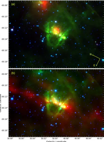
Fig. 1.Morphology of a bipolar HIIregion in the Spitzer bands. Red is
the MIPSGAL image at 24 µm, green is the GLIMPSE image at 8.0 µm, and blue is the GLIMPSE image at 4.5 µm.
energy distribution (SED) of each pixel is then fitted by a single-temperature modified black-body model. No background emission is subtracted from the images prior to the SED fitting. Thus, the temperature maps represent the mean temperature for all material along the line of sight, weighted by the intensity of the emission. The dust opacities adopted for the SED fitting are κν = 35.2, 14.4, 7.3, and 3.6 cm2g−1 at 160, 250, 350, and
500 µm, respectively (see Table 1 ofDeharveng et al. 2012, and discussions therein). Uncertainties on derived dust temperatures are on the order of 2 K, mainly due to the uncertainty in the dust opacities (see discussion in Paper I).
We use the temperature maps to obtain high-resolution col-umn density maps. We regrid the temperature maps to the resolution of the 250 µm data (1800), then estimate the column
density using the intensity of the 250 µm map, the temperature from the regridded temperature map, and Eq. (2) of Paper I. We assume that the regridded temperature does not differ strongly from the one that would be obtained if all the maps had the resolution of the 250 µm observations.
We stress that the column density of a structure can depend upon its size. For example, if the size of a structure (a clump, a core, a filament) is smaller than 1800, then this structure is
smoothed out in our maps and its peak column density is under-estimated; this effect can be important for distant regions1 (see
also discussions inBaldeschi et al. 2017). 2.2. Characterisation of dust clumps
As in Paper I, for each region we only discuss the highest column density structures. We estimate the mass of the central region of such structures by integrating the column density in an aperture following the level at the column density peak’s half intensity. Although this approach is more suitable for compact clumps, it is interesting for two reasons: 1) if the clump can be approximated
1 Consider, for example, a core and a clump that can be modelled as
Gaussians of FWHM 0.1 and 0.5 pc, respectively. At 1, 2, and 5 kpc the peak column density of the core will be reduced by factors of 0.57, 0.25, and 0.05 due to the smoothing by the beam. At 1, 2, 5, and 8 kpc the peak column density of the clump will be reduced by factors of 0.97, 0.89, 0.57, and 0.34.
by an elliptical Gaussian of uniform temperature, its total mass is twice the mass measured using an aperture following the level at half the peak’s value; and 2) the derived mass is not depen-dent on the beam size, which therefore allows us to compare the masses (and mean density) of clumps at different distances and angular sizes. We estimate the mean volume density in the central regions of the clumps, using their mass and beam decon-volved size obtained for the aperture following the level at half the maximum value, assuming a spherical morphology and a homogeneous medium.
While estimating the parameters of the dense structures, we have subtracted a background column density value, which we estimate from regions close to the structures. This is done to minimise the effects of emission along the line of sight.
2.3. Search for ionised region and associated exciting star or cluster
We use Hα maps (from the SuperCOSMOS survey) and radio-continuum maps (from the NVSS, VGPS, and SUMSS surveys) to search for emission from the ionised gas in the central region of the bipolar HIIregions. We then search for the exciting stars
within the central ionised region of each bipolar nebula. The best way to identify O- and early B-type stars is through spec-trophotometry, but these data do not exist for most of the bipolar nebulae in our sample. We therefore use two other methods:
(i) When the distance to the bipolar nebula is known but the exciting star is not (possibly due to high extinction), we use the radio continuum flux of the HIIregion to estimate
the likely spectral type of the probable ionising star. Using Eq. (1) inSimpson & Rubin (1990), and assuming an elec-tron temperature of 8000 K for the HII region and a ratio
He+/H+ = 0.05, we estimate the ionising photon flux, and
spectral type adopting the calibration ofMartins et al.(2005) for O stars and ofSmith et al.(2002) for early B stars. Here we assume that the exciting star is single and that no ionising photons are absorbed in the ionised region or leaked out into the interstellar medium (ISM).
(ii) When the distance to the HII region is known and the
exciting cluster is visible, we use the near-infrared (NIR) cat-alogues to identify the exciting star (see Fig. 3 of Paper I). The exciting cluster can be undetectable in the NIR if it is hidden behind dense filamentary cloud located along the line of sight, at the waist of the nebula. The spectral types of massive stars derived using NIR data can be uncertain, par-ticularly if the stars have excess emission in the NIR bands. To minimise the effect of excess emission, we mostly use J-band luminosity of the potential sources. We use the abso-lute magnitudes and colours ofMartins & Plez (2006) to characterise O-type stars. For less massive stars, we use the data table ofPecaut & Mamajek (2013). When possible, we use both the above criteria to determine the distance to the bipolar HII regions (e.g. see discussion in the Sect. 6.1 of
Paper I).
2.4. Classification and characterisation of young stellar objects
In this work, we are interested in tracing recent star formation around bipolar HIIregions. We therefore use the following indi-cators to search for Class 0, Class I, and flat-spectrum young stellar objects (YSOs) in their vicinities:
– [3.6]–[4.5] vs. [5.8]–[8.0] colour–colour diagram (Megeath
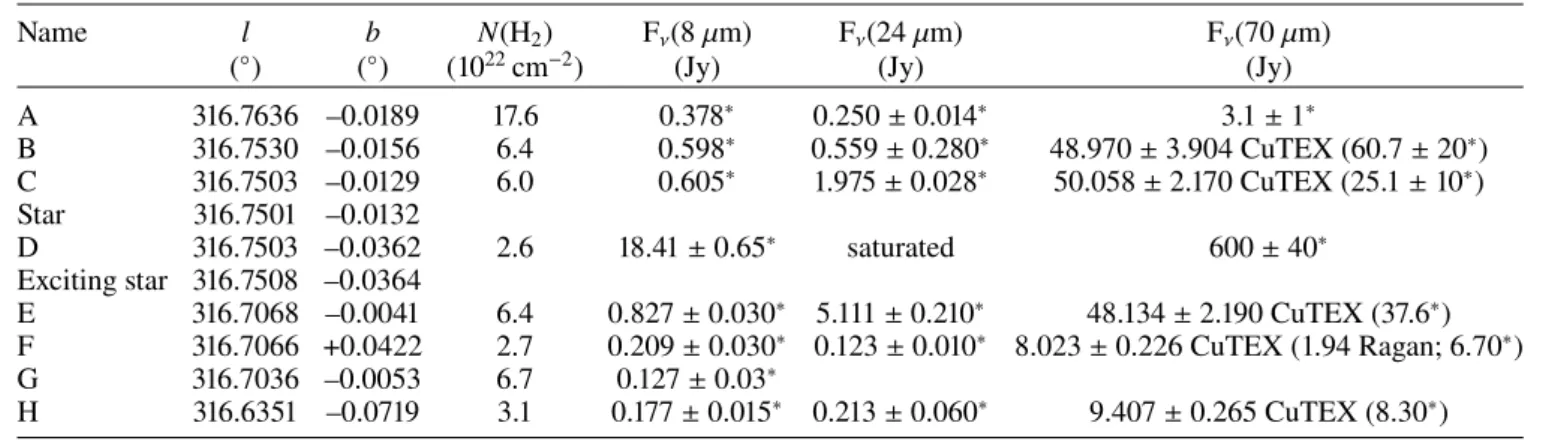
Fig. 2.Unsharp-masked images of G049.99–00.13 at 70, 24, and 8 µm.
catalogue. We use this diagram mainly to identify candidate Class I YSOs, and also to understand the evolutionary sta-tus of some of the bright sources that coincide positionally with the dense structures of the bipolar fields. We note that this IRAC colour–colour diagram was first established for sources corrected for extinction (e.g. seeAllen et al. 2004), which is not the case for the bipolar HIIregions presented
here. As a consequence of the high extinction, Class II YSOs in the IRAC colour–colour diagram can be found in the area generally attributed to Class I YSOs.
– We use 24 µm data from the Spitzer-MIPSGAL catalogue to confirm this first classification. To better distinguish between Class I, flat-spectrum, and Class II YSOs, we use the colour [8.0]–[24], which is less affected by extinction compared to IRAC colours. Class I sources have [8.0]–[24] ≥ 3.9, Class II have [8.0]–[24] ≤ 3.2, and flat-spectrum sources of uncertain nature between Class I and Class II lie in between. We sug-gest that the identification and classification of those IRAC sources that have no 24 µm measurements are likely more uncertain (more details can be found in Paper I).
– We use Herschel 70 µm data to search for Class 0 sources. In the Orion complex,Stutz et al.(2013) found 18 sources that are detected only at wavelengths ≥70 µm, but that have characteristics of early Class 0 sources. A Class 0 object could have a 24 µm counterpart, but not an NIR one. Since a strong correlation between the bolometric luminosity and the 70 µm flux has been found for protostars (Dunham et al. 2008), when possible we also use the Herschel 70 µm flux to estimate luminosity of the YSOs (for details see Paper I, Sect. 4.3).
We note that evolved stars, such as asymptotic giant branch (AGB) stars, can also be found at the same locations as Class I/II YSOs in colour-based criteria. We expect that contamination of our YSO sample with AGB stars is minimal, because most AGB stars will still be found in the colour-space of Class III YSOs compared to the Class II/I YSOs. For example, in the Serpens cloud, 62% of the Class III sources and 5% of the Class II sources were found to be background AGB stars when examined through spectroscopic observations byOliveira et al.(2009), and a similar conclusion is reached byRomero et al.(2012).
A few interesting sources are missing in the GLIMPSE and MIPSGAL catalogues, and we add these to our catalogues manually. These are mostly sources located in the direction of the bright photon-dominated region (PDRs) surrounding HII
regions, and therefore evaded automated detection. We mea-sure the fluxes of these sources using point-spread function (PSF) fitting or aperture photometry. The latter is applied in the case of isolated sources superimposed on a relatively uniform
background. Our measurements are calibrated using isolated point sources in the field of the bipolar nebula (details are given inDeharveng et al. 2012).
2.5. Creation of unsharp-masked images to unveil faint structures
We create unsharp-masked images by subtracting median-filtered images from the original ones. We generally use a filter window size of 5 × 5 pixels. Unsharp-masked images (shown in Fig.2) are used to:
– show the limits of the ionised region, and especially the lim-its of the lobes. The lobes may be faint and this emission is enhanced in the unsharp-masked images (see 70 µm image of Fig.2);
– allow for the detection of faint point sources, partly hidden by a bright nebular background emission (see 24 and 8 µm images of Fig.2);
– understand the dynamics of the ionised gas. Unsharp-masked images, especially at 8 µm, often display filaments originating from the waist of the nebula, perpendicular to the parental filament (see 8 µm image of Fig.2). We suggest that these filaments result from the high-pressure ionised material flowing from the high-density central region present at the waist of the nebulae. This ionised flow carves the surrounding inhomogeneous molecular material.
3. Results
In the following, we present a catalogue of the identified bipolar HIIregions, describe their global morphologies, and discuss the nature of the identified stellar and protostellar sources and dust clumps.
3.1. Catalogue of candidate bipolar HIIregions
Using the methodology described in Sect.2, we identify 16 bipo-lar HIIregions in the zone of the Galactic plane between ` ± 60◦
and |b| < 1◦ (240 square degrees). Table1 presents the
candi-date bipolar HIIregions. Column 1 gives their names (mainly
the name of the central radio HIIregions), Cols. 2 and 3 give
their central coordinates, Col. 4 their distances, Col. 5 the spec-tral type of their exciting stars if estimated or known, and Col. 6 contains some comments on individual HIIregions.
The morphology and various components of star-formation of the bipolar nebulae G319.88 + 00.79 and G010.32–00.15 were discussed in Paper I, whereas G049.99–00.13, G316.80–00.05, G320.25 + 00.44, G338.93–00.06, G339.59–00.12, and
Table 1.Candidate bipolar nebulae.
Name l b Distance Exciting star Comments [◦] [◦] [kpc] G004.40+ 00.11 004.404 +00.109 14.7 G008.14+ 00.23 008.138 +00.231 3.2 G010.32–00.14 010.317 –00.136 1.75 O5V–O6V Paper I G018.66–00.06 018.660 –00.059 3.8 G025.38–00.18 025.380 –00.181 5.2 G049.99–00.13 049.998 –00.125 7.94 O7V AppendixA G051.61–00.36 051.610 –00.357 5.3 G316.80–00.05 316.808 –00.037 2.8 O4V AppendixB G319.88+ 00.79 319.874 +00.770 2.6 O7V–O8V Paper I G320.25+ 00.44 320.247 +00.443 2.1 O8.5V–O9V AppendixC G330.04–00.06 330.039 –00.057 2.6 G331.26–00.19 331.266 –00.193 5.3 G338.93–00.06 338.929 –00.063 3.1 O7V–O7.5V AppendixD G339.59–00.12 339.578 –00.124 2.8 O7.5V AppendixE G342.07+ 00.42 342.085 +00.423 4.7 O5.5V–O6V AppendixF G356.35+ 00.22 356.351 +00.224 G342.07 + 00.42 are fully discussed in the Appendices of this work. Details concerning the remaining regions will be the subject of a future paper.
3.2. The global morphology of the bipolar HIIregions
Based on our findings (discussed in Appendices), Fig.3shows a schematic global view of a star forming complex associated with a bipolar HIIregion. In general, the bipolar HIIregions are
com-posed of a parental filament or sheet, bisected by a central region of ionised gas, with two ionised lobes oriented perpendicular to the parental filament. In the following, we discuss our findings on the global morphology and physical condition of individual components of the ISM associated with the bipolar HIIregions. 3.2.1. The parental filament or sheet
Parental filaments are detected by Herschel-SPIRE (250– 500 µm), as they contain cold dust. As an illustration, see the temperature map of G319.88+00.79, an almost perfect bipolar nebula (Paper I, Fig. 7); the parental filament is cold, with a min-imum temperature of 13.4 K (the dust in the PDRs surrounding the two ionised lobes is warmer, with a maximum temperature of 23.2 K). The best examples of parental filaments are found in the G008.14+00.23, G018.66–00.06, G049.99–00.13, G051.61– 00.36, G316.790–0.045, G319.88+00.79, and G320.25+00.44 fields. All such regions have: i) cold dust in the filament far from the ionised region, with a temperature in the range 14–17 K; and ii) warmer dust in the PDR surrounding the ionised gas, with a temperature generally higher than 20 K.
We note that what we see as filament (e.g. Paper I, Fig. 7) is the projection in the plane of the sky of a thee-dimensional universe. Therefore, what appears as filamentary structures – what we refer to as the parental filaments – may be dense sheets of material viewed nearly edge-on (we stress that it is this configuration in theBodenheimer et al.(1979) simulation; Fig. 1 of Paper I). In this case, if the line of sight is slightly inclined with respect to the plane of the sheet, we expect to see the dense material at the waist of the bipolar nebula forming a torus. At 8 µm, the foreground side of the torus may be seen in absorption, whereas at SPIRE wavelengths an almost complete
Fig. 3.Overall morphology of a bipolar HIIregion and its environment. Pink highlights for the ionised gas, blue the molecular material, and grey shows PAH emission at 8.0 µm. Various sources are also represented. The two lobes are, in general, well traced at 8.0 µm; a wavelength band is dominated by the emission of PAHs located in the PDR surrounding the ionised gas. There is a dense filament, observed as a cold elongated high-column-density feature at the centre of the lobes. This structure appears in emission at Herschel-SPIRE wavelengths and in absorption at 8 and 24 µm.
torus should be observed in emission (if the angular resolution allows us to separate the two sides of the waist). The eccentricity of the elliptical structure gives the inclination of the line of sight with respect to the plane of the dense sheet (assuming a circular waist). Three of the presented bipolar nebulae have this configuration: G010.32–00.14 (inclination angle ∼37◦;
Paper I), G319.88+00.79 (inclination angle ∼32◦; Fig. 6 in
Paper I), and G338.93–00.06 (inclination angle ∼13◦; Fig.D.4).
For the three other nebulae studied in detail here, the follow-ing configuration is hinted at: G004.40+ 00.11, G320.25 + 00.44, and G342.07+00.42. Nine regions are clearly seen edge-on: G331.26–00.19. G008.14+ 00.23, G018.66–00.06, G025.38–00.18, G049.99–00.13, G051.61–00.36, G316.80– 00.05, G330.04–00.06, and G339.50–00.12.
The parental filaments appear as high-column-density struc-tures, with column densities higher than 1.5 × 1022cm−2 in
the presented regions2. We estimate the volume density in
the parental filaments from the zone of the filaments that is not affected by the HII regions. Such results are uncertain
because we do not know for sure whether the filaments are two-dimensional sheets or one-two-dimensional cylinders. We obtain a range for the mean density in the filaments by assuming both of these geometries. For example, in G316 (AppendixB) the den-sity is in the range 1.5–8 × 104cm−3, in G319 (Paper I) it is in
the range 1.6–8.0 × 104cm−3, and in G320 (AppendixC) it is
in the range 0.51–2.8 × 104cm−3.
3.2.2. The ionised central region
Since the column density is in general high in the central direc-tion of the bipolar HII regions, optical Hα emission is often
weak or undetectable, but free-free radio-continuum emission from the ionised gas is observed. In most cases, the ionised gas fills the central region and the two lobes. For example, Fig.4shows the NVSS radio emission of the bipolar HIIregion G008.14+00.23. The radio emission is elongated along the two lobes. Good agreement between the radio emission and the 24 µm emission in the central region can also be seen. The 24 µm emission is saturated in the direction of the peak of the radio emission. We find that these characteristics are common to most nebulae (Bania et al. 2010;Deharveng et al. 2012).
When we have radio continuum data with enough angular resolution (e.g. from the Multi-Array Galactic Plane Imaging Survey (MAGPIS) survey; Helfand et al. 2006), we often see that the emission is brighter in some zones around the waist of the nebulae; there, it comes from the dense ionised layers bor-dering the dense molecular condensations present at the waist. This is clearly the case in the bipolar HIIregions G010.32–00.14
(Paper I) and G316.80–00.05 (AppendixB). 3.2.3. The ionised lobes
The shape and extent of the lobes depend on the structure of the neutral medium surrounding the dense parental structure. We can trace the lobes using 8.0 µm emission, which borders the IFs. For most bipolar nebulae, the two lobes are of unequal size, which could be due to the combination of the difference in the density of the medium located on each side of the parental fil-ament and projection effects. The lobes can be characterised as being: i) small and closed (ionisation bounded) if expanding in a high-density medium, or ii) large if expanding in a low-density medium. It may even be open if the density of the surrounding medium is low, as in G010.32–00.15 (Paper I, Figs. 11 and 12).
Sometimes, we see several lobes of different sizes and/or ori-entations on the same side of the parental filament. We assume this is due to the fact that the IF expands more rapidly in some
2 This is possibly not characteristic of all bipolar HIIregion complexes
as the presence of a detectable parental filament is one of our selection criteria.
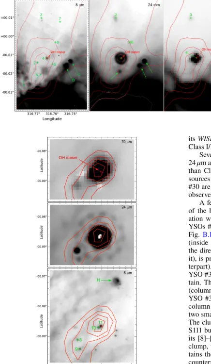
Fig. 4. Radio-continuum emission of G008.14+00.23. The Spitzer
24 µm (saturated in the centre) image (panel a) and the Herschel 70 µm image (panel b) over-plotted with 1.4 GHz contours from the NVSS survey (contour levels of 0.01, 0.05, 0.1, 0.5, 1.0, 1.5, 1.25, and 1.5 Jy beam−1). Panel c: colour composite image; red highlights the
radio emission at 20 cm from MAGPIS survey (in logarithmic units), green shows the 8 µm emission, and blue shows the unsharp 70 µm emission (to highlight the borders of the ionised lobes). The white con-tours indicate the NVSS radio emission (contour levels of 0.1, 0.5, and 1.0 Jy beam−1).
low-density channels, although we cannot ignore the possibil-ity of a burst of ionisation waves from the central massive stars. One example is G008.14+00.23, which has one small closed lobe and one larger faint lobe on the same side. Some regions show distorted lobes when the IF limiting the lobe meets a pre-existing dense condensation during its expansion; see for example Sh 201 of Deharveng et al. (2012) and its analogue in G342.07+00.42 (southern lobe, Fig.A.1) or G316.80–00.05 (southern lobe, Fig.B.1).
The dust in the PDRs bordering the ionised lobes is warm; generally warmer than 20 K and as high as 22–23 K. The G008.14+ 00.23 field illustrates this point as a dust temperature contour level of 20.75 K follows the border of the large northern lobe (Fig.5). The G316.80–00.05 field offers another example (Fig. B.3). Another characteristic of all our regions is that the warm dust is found in zones emitting at 8.0 µm (e.g. see Fig.B.3c or Fig.F.5c).
Sometimes the column density maps show the presence of molecular material surrounding the ionised lobes. Compared to the parental filaments, the column density is not usually high
Fig. 5.Large northern lobe of G008.14+00.23. The image is of Spitzer
8.0 µm data; the emission of the northern lobe has been enhanced using a logarithmic scaling. The green contour corresponds to a dust tem-perature of 20.75 K; it follows the PDR bordering the northern lobe (green arrow). The dashed red curve shows the position of the parental filament.
in these structures, in the range 1–3 × 1022cm−2 (background
subtracted). This is observed for example around the two small lobes of G008.14+00.23, around the bottom lobe of G049.99–00.13, and around the western lobe of G320.25+00.44. The best example, however, is found around the eastern lobe of G338.93–00.06 (Fig.D.3). We suggest that we are dealing with neutral material collected during the expansion of the lobes. 3.3. The global nature of central stars, YSOs, and clumps Figure3 gives a schematic of the various sources observed in the vicinity of the bipolar HIIregions: the exciting star or
clus-ter, YSOs, and clumps. Below we describe the global nature and properties of such sources.
3.3.1. The exciting central star or cluster
The identification of the stellar sources (e.g. the exciting star or cluster) allows for an estimate of the distance to the HIIregion;
G010.32–00.15 from Paper I illustrates this point. Prior to our study, the distance to this region was very uncertain, in the range of 2–19 kpc for kinematic distances. The spectral type of the exciting star is known, determined byBik et al.(2005). UKIDSS images of the region show the exciting cluster. Using NIR data of the exciting cluster we estimated its distance to be 1.75 kpc, close to the near kinematic distance.
The exciting star or cluster is expected to lie at the centre of the HIIregion. The region G319.88+00.79 presents an
exem-plary case of a central exciting cluster (Fig. 5 in Paper I); the cluster lies at the exact centre of the waist, at the centre of the elliptical ring. In this work, we have identified the most-likely exciting star (except for G316.80–00.05) in the central regions of the bipolar nebulae; in most cases, we do not see a cluster around them. In bipolar bubbles, this central region is gener-ally found in the direction of the parental filament, and therefore may be strongly affected by extinction. This is one of the possi-ble reasons for not being apossi-ble to identify the exciting cluster in most of the HIIregions. For example, we searched for the excit-ing cluster of G320.25+00.14 and G316.80–00.05, but we were not able to conclusively identify them. Similarly, we do not see any stellar cluster in the central region of G004.40+00.11 and G008.14+00.23.
Fig. 6.Identified Class I YSOs in the field of bipolar nebulae, using two
indicators. The underlying diagram is that of the region G316.80–00.05 (Fig.B.9), although the diagram of any other region could have been used. The colours give the nature of these sources according to their [8]–[24] colours. Green, blue, and black circles identify Class I, flat-spectrum, and Class II YSOs, respectively. Black “X” sources are for probable evolved stars. Small red dots are for sources of unknown nature because their 24 µm magnitude is unknown. The extinction law is that ofIndebetouw et al.(2005).
3.3.2. The evolutionary status of the YSOs
We use two different indicators to identify YSOs: GLIMPSE [3.6]–[4.5] vs. [5.8]–[8.0] colours and [8]–[24] colours. As underlined in Sect.2.4, the GLIMPSE [3.6]–[4.5] vs. [5.8]–[8.0] diagram is sensitive to the extinction, whereas the [8]–[24] colour is less sensitive. In Fig. 6, we compare the results obtained with the above two indicators. We are interested only in sources located in or close to the zone defined for Class I sources in the GLIMPSE colour–colour diagrams. Figure 6
shows the results obtained for 84 GLIMPSE Class-I sources with [8]–[24] colour, located in the fields of G010.32–00.14, G018.66–00.06, G049.99–00.13, G316.80–00.05, G319.88+ 00.79, G320.25+ 00.44, G338.93–00.06, and G339.59–00.12. Based on their [8]–[24] colours, they have been classified into different evolutionary stages and are shown in different colours in Fig. 6. The small red dots in the Class I zone are for sources of unknown nature; they have no 24 µm measure-ments, because they are either saturated or not detected at 24 µm. Of the IRAC-identified Class I YSOs that have 24 µm detections, we find that 28 are Class I (the two indicators agree), 25 are flat-spectrum, and 12 are Class II based on their [8]–[24] colours. This analysis shows the difficulty in disen-tangling Class I and Class II YSOs based on GLIMPSE data only, and thus the need for high-resolution longer-wavelength observations. Nonetheless, we can say that roughly 80% of the IRAC-classified Class I sources should be protostellar (i.e. Class I and spectrum). The lifetime of Class I and flat-spectrum sources are of the order 105yr; therefore, the presence
of such sources suggests recent star formation activity in the region.
Fig. 7.Mass of the clumps associated with
bipo-lar nebulae, observed either around their waists or along the parental filaments.
Fig. 8.Mean volume density of the clumps associated with bipolar nebulae, observed either around their waists or along the parental filaments.
The black circles indicate clumps containing a source more luminous than 1000 L . The red line on the low-density side indicates the range of
densities estimated for the parental structures.
3.3.3. Location and properties of molecular clumps
Massive clumps are always present at the waist of the nebulae; they are part of the parental structure. The clumps found adjacent to the ionised regions are always the most massive, compact, and dense structures in the vicinity. We do not compare their peak column densities as these values depend on their angular sizes as compared to the resolution of the 250 µm observations. We do, however, compare their mass and mean volume densities of the central regions assuming that shape of the clumps is Gaussian in nature, and therefore their total mass is twice that of the central regions (see discussion in Sect.2.2).
Figure7shows the masses of these clumps, which lie in the range 200 M –1400 M . We observe no relationship between the
mass of the clumps and ionising source of the central nebulae. We suggest instead that the observed mass of the clumps strongly depends on the density and structure of the parental clouds, star-formation activity within the clumps, and/or the age of the central bipolar nebulae (if formed by collect-and-collapse-like process, then older sources are expected to collect more material; see discussion inDeharveng et al. 2010).
Figure 8 displays the mean density of the central regions of the clumps. The density can be as high as a few 106cm−3.
Globally, the density of clumps containing a luminous source (massive YSOs or ultra-compact (UC) HII regions) is higher
than that of clumps devoid of luminous sources. It therefore seems that for these regions massive stars form in dense clumps rather than in massive ones.
Infrared dark clouds (IRDCs) are often described as the loca-tions where star formation occurs. Based on Spitzer 8 µm opacity maps, Peretto & Fuller (2009) identified over 50 000 single-peaked IRDC fragments in our Galaxy, in the region of Galactic longitude and latitude 10◦ < |l| < 65◦ and |b| < 1◦. Many of
the massive and dense clumps inside which massive stars are forming are not reported as IRDC fragments by Peretto & Fuller(2009). Such clumps are not seen in absorption at Spitzer
wavelengths due to their locations near to HIIregions and their
PDRs, and therefore they are hidden by the bright emission of the PDRs. Many examples can be found:
– In the G010.32–00.14 (Paper I) field, three massive clumps (C1, C2, and C3 of mass 180, 223, and 330 M , respectively)
lie at the waist of nebula and are not IRDCs; they contain MYSOs (maser sources) of high luminosity (>1600 L ).
– In the G320.25+00.44 field (Appendix C), the most mas-sive (∼280 M ) clump, C1, has not been identified as an
IRDC despite being a strong absorption feature at 8.0 µm. It contains a source with a luminosity ∼1700 L .
– In the G339.58–00.12 field (Appendix E), two massive clumps (C1 of mass 550 M and C2 of mass 360 M ; see
Fig.E.4) are located at the waist of the nebula. C1 contains a MYSO of luminosity ∼2400 L which is not an IRDC, and
the IRDC detected in the vicinity of C2 (which contains a young cluster of 15 000 L ) lies far from the column density
peak.
We suggest in the field of HIIregions that Spitzer-based IRDC
fragments are not likely to be the best sites to search for massive star formation.
4. Star formation near bipolar HIIregions
This section discusses various components of the recent star-formation observed around the bipolar HII regions, and the possible existence of triggered star-formation in these regions. 4.1. Bright-rimmed clumps at the waist
Clumps located at the waist of bipolar nebulae are often sur-rounded by bright rims (BRs) that are bright at 8.0 µm. The BRs are observed on the clump-side adjacent to the ionised region. A Class I YSO is often located inside the clump, not towards its centre, but just behind the bright rim and very close to it.
Fig. 9.Star formation in two clumps located at the waist of G004.40+00.11. The stellar content of the clumps is shown by 4.5 µm (panel a), 8.0 µm
(panel b), and 70 µm (panel c) images. The over-plotted red contours are of column density (levels of 1.5, 1.0, 0.75, 0.5, 0.25 × 1023cm−2) and the
green contours are of 70 µm emission (levels of 20 000, 15 000, 10 000 MJy sr−1). Panel d: composite colour image with 70 µm emission in red, an
unsharp image of the 8.0 µm emission highlighting the bright rim bordering clump C2 in green, and 4.5 µm emission in blue. The orange arrows point to the two YSOs emitting at 70 µm. The green contours are of 70 µm emission.
We describe two such cases are as follows. The best example is from the bipolar nebula G316.80–00.05 (Fig.B.7). Two clumps, C1 and C2, are located close to the eastern waist of the neb-ula. The C1 clump (mass ∼ 1360 M , density ∼ 7.4 × 105cm−3)
is bordered by a BR on its face turned towards the ionised region. This BR is also a dense ionised layer (it displays arc-like radio emission). Behind the BR, at ∼0.03 pc in projection, lies a hydroxyl (OH), water (H2O), and methanol (CH3OH) maser
that is also coincident with an EGO with jets. This is therefore a Class I YSO. The luminosity of this source is estimated to be ∼26 000 L . The resolution of the radio emission does not allow
us to separate the emission of the BR and that of the massive YSOs forming nearby.
The bipolar nebula G004.40+00.11 is another example that has bright rim clumps. Two clumps, C1 and C2, are located at the northern extremity of the waist. Each clump contains a YSO (see Fig.9). The C2 clump is located adjacent to the HIIregion.
It is warm and surrounded by a bright rim. Wide-field Infrared Survey Explorer (WISE;Wright et al. 2010) photometry suggests that the source embedded in C2 is a Class I YSO. The 4.5 µm image shows the presence of faint extended emission close to the YSO; we suggest that it is likely due an outflow activity such as those found in EGOs (e.g.Cyganowski et al. 2008). It lies very close to the bright rim (∼2.006 in projection).
In some other regions, the YSO is rather far from the BR, but not in the very centre of the clump. One example is the G010.32–00.14 bipolar HIIregion (Paper I, Fig. 23). The central clumps, C2 and C3, are bordered on their side facing the exciting cluster by BRs observed both at 8.0 µm and at radio wavelengths
(in the MAGPIS survey images). They contain massive young sources. For example, C1 contains a massive Class I YSO of high luminosity (4600 L ; associated with a methanol maser), while
C2 contains a UC HIIregion. These two sources do not lie at
the centre of the clumps. Another example is the G338.93–00.06 region, which has an elliptic waist (AppendixD) with a bright clump (C1: mass ∼275 M , density ∼2.7 × 106cm−3) bordered
by a BR. Behind the BR, at about 0.1 pc in projection (at equal distance between the BR and the column density peak) lies an IR source associated with a methanol maser. This source is bright at 70 µm, with a luminosity of ∼4500 L .
4.2. Possible second-generation young clusters
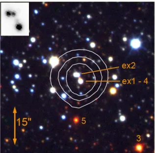
Young clusters (small groups of Class I YSOs or IR point sources as opposed to isolated point sources) are observed in the follow-ing two regions. Firstly, the G339.59–00.12 field (AppendixE). Two massive and dense clumps, C1 and C2, are observed at the waist of the nebula (see Fig. E.4). Massive-star forma-tion is observed in each of them. The C1 clump (mass ∼ 550 M , density ∼6.2 × 105cm−3; Fig.10) contains a small group
of Class I and flat-spectrum YSOs (at least 4 Class I), an EGO, and a methanol maser. Secondly, the G342.07+00.42 field (AppendixF). Two massive and dense clumps, C1 and C2, are observed at the waist of the nebula (see Fig.F.4). The C1 clump (mass ∼ 1030 M , density ∼ 2.9 × 105cm−3) lies on the west
side of the waist. On VISTA images, a tight cluster seems to be embedded in C1 (Fig.11). The clump contains a UC HIIregion
Fig. 10.Colour composite image showing the second-generation cluster
of G339.59–00.12. The image is made with Spitzer 8.0 µm (red), 4.5 µm (green), and VISTA Ks (blue) data. The red contours are for column
densities of 0.5 × 10²³and 1.0 × 1023cm−2.
Fig. 11.Colour composite image showing the second-generation
clus-ter of G342.07+00.42. The image is made with VISTA J- (blue), H- (green), and K-band (red) images. The red contours are for column densities of 0.5 × 10²³, 1.0 × 10²³, and 1.5 × 1023cm−2. The two orange
arrows point to probable candidate exciting stars.
Since UC HII regions and masers trace very early phases
(≤105yr) of star formation. We suggest that these clusters are
likely second-generation clusters of the field. 4.3. Small diffuse regions
Small diffuse regions of extended 8.0, 24, and 70 µm emission are often observed in the vicinity of bipolar nebulae. These extended regions are much smaller in size compared to the bipolar HII regions (e.g. 0.25 vs. 3.8 pc for region D in the
field of G316.80–0.05). A star is often present in the centre of these regions. Based on these stars’ brightnesses and the lack of detected free-free emission from ionised gas, the stars may be of spectral type B. For example, in the field of G049.99–00.13
(AppendixA), three such regions are present. Two regions are located along the parental filament, in a condensation adjacent to the ionised region, and behind a bright rim; they are there-fore likely associated with the bipolar nebula. In G339.59–00.12 (AppendixE), four small regions are present. Two of them con-tains stars. In the field of G316.80–00.05 (AppendixB), seven such regions are observed.
We suggest that these presumed B-type stars heat the dust and excite PAHs in their surroundings. We would require deep high-resolution radio observations to determine if the stars are massive enough to ionise their surroundings and form UC HII regions. Only in the case of G010.32–00.14 (Paper I;
MAGPIS observations) we know the presence of a UC HII
region.
We have no information on the evolutionary status of most of these regions. At longer wavelengths these sources are extended, and therefore we cannot conclusively say whether they are of the same generation as the exciting stars of the bipolar nebulae or if they represent second-generation massive stars. Only in the case of the UC HIIregion in G010.32–00.14 we suggest that we are
looking at a second-generation massive source, as it is embed-ded inside a clump compressed by the adjacent central nebula. Spectroscopic observations would reveal the true nature of these sources.
4.4. Triggered star formation
In the studied regions, several observational signatures point to star formation triggered by the central expanding bipolar HII
regions.
The most massive clumps in all our fields are without excep-tion adjacent to the central ionised region. We cannot exclude that a few of them were pre-existing along the parental filament or in the parental sheet, but we regard it as probable that all of them were pre-existing as very low. How did these clumps form? We suggest that they formed from collected material as the ionised region expanded into the dense material of the parental filament or sheet. The morphology of the G010.32–00.14 com-plex (Paper I) is consistent with this interpretation, as there are five massive clumps surrounding the waist of the bipolar neb-ula. Again, we regard the probability of finding five pre-existing clumps surrounding an HII region and reached by the IF at
the same time as very low. A similar situation is observed in G338.93–00.06 where four condensations are distributed along the waist of the nebula (Fig.D.3).
We know that a very early phase of star formation is at work in these clumps because Class 0/I sources, often associated with class II methanol masers, are detected in the direction of these clumps. In a few cases, we observe these sources close to the IF. This suggests that they form in the high-density compressed layer bordering the IF. High-angular-resolution molecular obser-vations would allow us to better determine the morphology of the clumps in the vicinity of the IF.
We note that this type of star formation, that we believe was triggered by the expansion of central HII region, leads
to the formation of luminous (and therefore probably massive) sources (see Fig.8). One extreme example is the UC HIIregion
embedded in clump C3 in the G010.32–00.14 field. Another extreme case is the source embedded in the C1 clump in the G316.804–400.05 field, which has a luminosity of ∼26 000 L
and is observed very close to the IF. The central bipolar HII
regions in these two cases have the highest excitation degree of the sample (they are ionised by O4–O6 stars).
In a few cases, we observe collected material surrounding the lobes, but no stars are forming there3. The column density
of this material is rather low, of the order of a few 1021cm−2,
much lower than that of the parental filamentary structure. This is probably the reason why no star formation is observed there.
We also observe star formation in pre-existing clumps reached by the IF limiting the lobes (C6 on the border of the bottom lobe in G010.32–00.14 and C5 on the border of the right lobe in G338.93–00.06; each shows star formation presently at work). In these cases, we do not know if star formation has been triggered by the compression of the clump by the high pressure ionised gas, or if star formation was already at work before the compression.
5. Conclusions
In this work, we studied six bipolar HIIregions at NIR,
mid-infrared (MIR), FIR, and radio wavelengths to determine their morphologies, parental cloud structures, and their impact on star formation in their vicinities. Our main conclusions are:
1. Massive clumps are present at the waist of bipolar HII
regions, adjacent to the ionised gas in all cases. They are massive, with several hundred solar masses in their cen-tral regions. High densities are found there, higher than 105cm−3, and up to several 106cm−3.
2. Massive Class I YSOs are frequently associated with masers in these clumps. The more luminous ones lie in the densest clumps. Some clumps also contain small clusters of Class I YSOs.
3. The massive YSOs are generally not located – in projection – at the centres of the clumps, but instead are found near the bright rims bordering the clumps on their faces towards the ionised gas. In some cases, they lie very close to the IF, prob-ably in or close to the layer of compressed material bordering the IF.
4. Star formation also occurs in some pre-existing condensa-tions reached by the IF during the expansion of the ionised lobes.
5. Points 1, 2, and 3 show that star formation has likely been triggered by the expansion of the central bipolar HIIregions.
As most of the massive YSOs are found at the waist of bipolar regions, this implies that recent star formation is mainly occurring in the material collected from the dense parental structures and not from the lower-density surround-ing medium (therefore from material collected in the dense parental structure, and not in the material collected around the lobes).
We have covered the area located between longitude –60◦ and
+60◦, latitude –1◦ and+1◦. This area contains about 1377 large
bubble HII regions (Simpson et al. 2012). By eye, we have
only identified 16 bipolar HII regions; even if this number is
underestimated by a large factor (mainly because we identify mostly bipolar HII regions seen edge-on) it is several hundred
times smaller than the number of bubble HII regions identi-fied by Simpson et al. (2012). This suggests that most of the bubble HII regions in our Galaxy are probably not formed in
two-dimensional, flat or sheet-like clouds.
The cloud structure that is at the origin of the bubble HII
regions remains to be understood. Modelling and numerical simulations of bipolar HIIregions are missing, although a very
3 A possible exception is the G338.93–00.06 field where two compact
sources are observed on the border of the left lobe, but we do not know whether or not they are associated with the bipolar nebula.
recent model byWhitworth et al.(2018) suggests that bipolar HII
regions can be created at the interface resulting from collisions between two clouds. More high-resolution simulations following the formation and evolution of an HIIregion excited by a
mas-sive star formed in a two-dimensional parental structure or inside a filament would shed light on their origin.
We also need to follow the formation of dense and massive clumps at the waist of the nebula, and the formation of massive sources inside these clumps. High-resolution molecular obser-vations of clumps with ALMA may help to understand exactly where star formation occurs, in the compressed layer adjacent to the IF as these first observations seem to indicate, or more embedded inside the clump.
Acknowledgements.We thank the anonymous referee for helpful and
construc-tive comments. The authors would first like to thank the Herschel Hi-GAL team for their continuing work on the survey. Observations were obtained with the Herschel-PACS and Herschel-SPIRE photometers. PACS was developed by a consortium of institutes led by MPE (Germany), including UVIE (Austria); KU Leuven, CSL, IMEC (Belgium); CEA, LAM (France); MPIA (Germany); INAF-IFSI/OAA/OAP/OAT, LENS, SISSA (Italy); IAC (Spain). This development was supported by the funding agencies BMVIT (Austria), ESA-PRODEX (Belgium), CEA/CNES (France), DLR (Germany), ASI/INAF (Italy), and CICYT/MCYT (Spain). SPIRE has been developed by a consortium of institutes led by Cardiff Univ. (UK) and including Univ. Lethbridge (Canada); NAOC (PR China); CEA, LAM (France); IFSI, Univ. Padua (Italy); IAC (Spain); Stockholm Observatory (Sweden); Imperial College London, RAL, UCL-MSSL, UKATC, Univ. Sussex (UK); Caltech, JPL, NHSC, Univ. Colorado (USA). This development was sup-ported by national funding agencies: CSA (Canada); NAOC (PR China); CEA, CNES, CNRS (France); ASI (Italy); MCINN (Spain); SNSB (Sweden); STFC and UKSA (UK); and NASA (USA). This paper uses data form VISTA Vari-ables in the Vía Láctea survey, obtained with VIRCAM/VISTA at the ESO Paranal Observatory. The VVV Survey is supported by BASAL Center for Astrophysics and Associated Technologies CATA PFB-06, by the Ministry of Economy, Development, and Tourism’s Millennium Science Initiative through grant IC12009, awarded to The Millennium Institute of Astrophysics (MAS). This publication makes use of data from The UKIRT Infrared Deep Sky Survey or UKIDSS which is a next generation near-infrared sky survey using the wide field camera (WFCAM) on the United Kingdom Infrared Telescope on Mauna Kea. This publication also made use of data products from the Two Micron All Sky Survey (a joint project of the University of Massachusetts and the Infrared Processing and Analysis Center / California Institute of Technology, funded by NASA and NSF. This paper also uses data observations made with the Spitzer Space Telescope (operated by the Jet Propulsion Laboratory, California Institute of Technology under a contract with NASA). We thank the French Space Agency (CNES) for financial support.
References
Acker, A., Chopinet, M., Pottash, S. R., & Stenholm, B. 1987,A&AS, 71, 163
Allen, L. E., Calvet, N., D’Alessio, P., et al. 2004,ApJS, 154, 363
Anathpindika, S., & Freundlich, J. 2015,PASA, 32, e007
Anderson, L. D., Bania, T. M., Balser, D. S., & Rood, R. T. 2011,ApJS, 194, 32
Anderson, L. D., Bania, T. M., Balser, D. S., & Rood, R. T. 2012,ApJ, 754, 62
Anderson, L. D., Bania, T. M., Balser, D.S., et al. 2014,ApJS, 212, 1
Anderson, L. D., Hough, L. A., Wenger, T. V., et al. 2015,ApJ, 810, 42
André, P., Men’shchikov, A., Bontemps, S., et al. 2010,A&A, 518, L102
André, P., Di Francesco, J., Ward-Thompson, D., et al. 2014,Protostars and
Planets VI(Arizona: University of Arizona Press), 27 Arthur, S. J., & Hoare, M. G. 2006,ApJS, 165, 283
Arzoumanian, D., Andrè, Ph., Didelon, P., et al. 2010,A&A, 529, L6
Avedisova, V. S., & Kondratenko, G. I. 1984,Ninfo, 56, 59
Baldeschi, A., Molinari, S., Elia, D., Pezzuto, S., & Schisano, E. 2017,MNRAS, 472, 1778
Bally, J., Snell, R. L., & Predmore, R. 1983,ApJ, 272, 154
Bania, T. M., Anderson, L. D., Balser, D. S., & Rood, R. T. 2010, ApJ,
718, L106
Beaumont, C. N., & Williams, J. P. 2010,ApJ, 709, 791
Bernard, A., Neichel, B., Samal, M. R., et al. 2016,A&A, 592, A77
Bica, E., Dutra, C. M., Soares, J., & Barbuy, B. 2003,A&A, 404, 223
Bieging, J. H., Peters, W. L., & Kang, M. 2010,ApJS, 191, 232
Bik, A., Kaper, L., Hanson, M. M., & Smits, M. 2005,A&A, 440, 121
Breen, S. L., Ellingsen, S. P., Caswell, J. L., & Lewis, B. E. 2010,MNRAS, 401, 2219
Bronfman, L., Nyman, L.-A., & May, J. 1996,A&AS, 115, 81
Busfield, A. L., Purcell, C. R., Hoare, M. G., et al. 2006,MNRAS, 366, 1096
Carey, S. J., Noriega-Crespo, A., Mizuno, D. R., et al. 2009,PASP, 121, 76
Caswell, J. L. 1996,MNRAS, 279, 79
Caswell, J. L. 1998,MNRAS, 297, 215
Caswell, J. L. 2001,MNRAS, 326, 805
Caswell, J. L., & Haynes, R. F. 1987,A&A, 171, 261
Caswell, J. L., Batchelor, R. A., Forster, J. R., & Wellington, K. J. 1989,Austr. J. Phys., 42, 331
Caswell, J. L., Vaile, R. A., Ellingsen, S. P., et al. 1995a,MNRAS, 272, 96
Caswell, J. L., Vaile, R. A., Ellingsen, S. P., & Norris, R. P. 1995b,MNRAS, 274, 1126
Chen, X., Ellingsen, S. P., Shen, Z.-Q., et al. 2011,ApJS, 196, 9
Churchwell, E., Povich, M. S., Allen, D., et al. 2006,ApJ, 649, 7597
Churchwell, E., Watson, D. F., Povich, M. S., et al. 2007,ApJ, 670, 428
Culverhouse, T., Ade, P., Bock, J., et al. 2011,ApJS, 195, 8
Cyganowski, C. J., Whitney, B. A., Holden, E., et al. 2008,AJ, 136, 2391
Cyganowski, C. J., Koda, J., Rosolowsky, E., et al. 2013,ApJ, 764, 61
Dale, J. E., Bonnell, I. A., & Whitworth, A. P. 2007,MNRAS, 375, 1291
Dale, J. E., Haworth, T. J., & Bressert, E. 2015,MNRAS, 450, 1199
Deharveng, L., Schuller, F., Anderson, L. D., et al. 2010,A&A, 523, A6
Deharveng, L., Zavagno, A., Anderson, L. D., et al. 2012,A&A, 546, A74
Deharveng, L., Zavagno, A., Samal, M.R., et al. 2015,A&A, 582, A1(Paper I) de Geus, E. J., Bronfman, L., & Thaddeus, P. 1990,A&A, 231, 137
Dobashi, K. 2011,PASJ, 63, 1
Dunham, M. M., Crapsi, A., Evans, N. J., et al. 2008,ApJS, 179, 249
Dutra, C., & Bica, E. 2002,A&A, 383, 631
Dutra, C. M., Bica, E., Soares, J., & Barbuy, B. 2003,A&A, 400, 533
Dyson, J. E., & Williams, D. A. 1997, inThe Physics of the Interstellar Medium, 2nd ed.(Bristol: Institute of Physics Publishing)
Ellsworth-Bowers, T. P., Rosolowsky, E., Glenn, J., et al. 2015,ApJ, 799, 29
Eswaraiah, C., Lai, S.-P., Chen, W.-P., et al. 2017,ApJ, 850, 195
Fontani, F., Cesaroni, R., & Furuya, R. S. 2010,A&A, 517, A56
Foster, J. B., Jackson, J. M., Barnes, P. J., et al. 2011,ApJS, 197, 25
Foster, J. B., Rathborne, J. M., Sanhueza, P., et al. 2013,PASA, 30, e038
Franco, J., Tenorio-Tagle, G., & Bodenheimer, P. 1990,ApJ, 349, 126
Fukuda, N., & Hanawa, T. 2000,ApJ, 533, 911
Gardner, F. F., & Whiteoak, J. B. 1978,MNRAS, 183, 711
Georgelin, Y. M., Boulesteix, J., Georgelin, Y. P., et al. 1987,A&A, 174, 257
Georgelin, Y. M., Russeil, D., Marcelin, M., et al. 1996,A&AS, 120, 41
Goedhart, S., Gaylard, M. J., & van der Walt, D. J. 2004,MNRAS, 355, 553
Goldsmith, P. F., Heyer, M., Narayanan, G., et al. 2008,ApJ, 680, 428
Green, J. A., & McClure-Griffiths, N. M. 2011,MNRAS, 417, 2500
Green, J. A., Caswell, J. L., Fuller, G. A., et al. 2010,MNRAS, 409, 913
Gvaramadze, V. V., Kniazev, A. Y., & Fabrika, S. 2010,MNRAS, 405, 1047
Hartley, M., Tritton, S. B., Manchester, R. N., et al. 1986,A&AS, 63, 27
Helfand, D. J., Becker, R. H., White, R. L., Fallon, A., & Tuttle, S. 2006,AJ, 131, 2525
Henney, W. J., Arthur, S. J., & García-Díaz, M. T. 2005,ApJ, 627, 813
Hill, T., Motte, F., Didelon, P., et al. 2011,A&A, 533, A94
Hosokawa, T., & Inutsuka, S.-I. 2005,ApJ, 623, 917
Huang, M., Bania, T. M., Bolatto, A., et al. 1999,ApJ, 517, 282
Hughes, V. A., & MacLeod, G. C. 1994,ApJ, 427, 857
Indebetouw, R., Mathis, J. S., Babler, B. L., et al. 2005,ApJ, 619, 931
Jackson, J. M., Finn, S. C., Rathborne, J. M., et al. 2008,ApJ, 680, 349
Jackson, J. M., Rathborne, J. M., Foster, J. B., et al. 2013,PASA, 30, e057
Kahn, F. D., & Dyson, J. E. 1965,ARA&A, 3, 47
Kang, M., Bieging, J. H., Povich, M. S., & Lee, Y. 2009,ApJ, 706, 83
Koenig, X. P., Leisawitz, D. T., Benford, D. J., et al. 2012,ApJ, 744, 130
Könyves, V., André, P., Men’shchikov, A., et al. 2015,A&A, 584, A91
Kothes, R., & Dougherty, S. 2007,A&A, 468, 993
Kothes, R., & Dougherty, S. 2008,Rev. Mex. Astron. Astrof., 33, 163
Kuchar, T. A., & Clark, F. O. 1997,ApJ, 488, 224
Lawrence, A., Warren, S. J., Almaini, O., et al. 2007,MNRAS, 379, 1599
Lee, E. J., Murray, N., & Rahman, M. 2012,ApJ, 752, 146
Liu, H.-L., Li, J.-Z., Wu, Y., et al. 2016,ApJ, 818, 95
Lockman, F. J. 1989,ApJS, 71, 469
Longmore, S. N., Burton, M. G., Barnes, P. J., et al. 2007, MNRAS,
379, 535
Martins, F., & Plez, B. 2006,A&A, 457, 637
Martins, F., Schaerer, D., & Hillier, D. J. 2005,A&A, 436, 1049
Marsh, K. A., Kirk, J. M., André, P., et al. 2016,MNRAS, 459, 342
Mc Gee, R. X., & Newton, L. M. 1981,MNRAS, 196, 889
Megeath, S. T., Allen, L. E., Gutermuth, R. A., et al. 2004,ApJS, 154, 367
Mercer, E. P., Clemens, D. P., Meade, M. R., et al. 2005,ApJ, 635, 560
Minier, V., Tremblin, P., Hill, T., et al. 2013,A&A, 550, A50
Minniti, D., Lucas, P. W., Emerson, J. P., et al. 2010,New Astron., 15, 433
Mizuno, A., Onishi, T., Yonekura, Y., et al. 1995,ApJ, 445, L161
Molinari, S., Swinyard, B., Bally, J., et al. 2010a,PASP, 122, 314
Molinari, S., Swinyard, B., Bally, J., et al. 2010b,A&A, 518, L100
Molinari, S., Schisano, E., Faustini, F., et al. 2011,A&A, 530, A133
Motte, F., Bontemps, S., & Louvet, F. 2018,ARA&A, in press
Myers, P. C. 2009,ApJ, 700, 1609
Nowak, M., Flagey, N., & Noriega-Crespo, A. 2014,ApJ, 796, 116
Oliveira, I., Merín, B., Pontoppidan, K. M., et al. 2009,ApJ, 691, 672
Otrupek, R. E., Hartley, M., & Wang, J.-S. 2000,PASA, 17, 92
Panwar, N., Samal, M. R., Pandey, A. K., et al. 2017,MNRAS, 468, 2684
Parker, Q. A., Phillipps, S., Pierce, M. J., et al. 2005,MNRAS, 362, 689
Pavlyuchenkov, Y. N., Kirsanova, M. S., & Wiebe, D. S. 2013,Astron. Rep.,
57, 573
Pecaut, M. J., & Mamajek, E. E. 2013,ApJS, 208, 9
Pecaut, M. J., Mamajek, E. E., & Bubar, E. J. 2012,ApJ, 746, 154
Peretto, N., & Fuller, G.A. 2009,A&A, 505, 405
Raga, A. C., Cantó, J., & Rodríguez, L. F. 2012,MNRAS, 419, L39
Ragan, S., Henning, T., Krause, O., et al. 2012,A&A, 547, A49
Rieke, G. H., & Lebofsky, M. J., & Low, F. J. 1985,AJ, 90, 900
Robitaille, T. P., Meade, M. R., Babler, B. L., et al. 2008,AJ, 136, 2413
Rodgers, A. W., Campbell, C. T., & Whiteoak, J. B. 1960,MNRAS, 121, 103
Romero, G. A., Schreiber, M. R., Cieza, L. A., et al. 2012,ApJ, 749, 79
Samal, M. R., Zavagno, A., Deharveng, L., et al. 2014,A&A, 566, A122
Schneider, S., & Elmegreen, B. G. 1979,ApJS, 41, 87
Schutte, A. J., van der Walt, D. J., Gaylard, M. J., & MacLeod, G. C. 1993,
MNRAS, 261, 783
Shaver, P. A., Retallack, D. S., Wamsteker, W., & Danks, A. C. 1981,A&A, 102, 225
Simpson, J. P., & Rubin, R. H. 1990,ApJ, 354, 165
Simpson, R. J., Povich, M. S., Kendrew, S., et al. 2012, MNRAS, 424,
2442
Smith, L.J., Norris, R. P. F., & Crowther, P. A. 2002,MNRAS, 337, 1309
Skrutskie, M. F., Cutri, R. M., Stiening, R., et al. 2006,AJ, 131, 1163
Steggles, H. G., Hoare, M. G., & Pittard, J. M. 2017,MNRAS, 466, 4573
Strömgren, B. 1939,ApJ, 89, 526
Stutz, A. M., Tobin, J. J., Stanke, T., et al. 2013,ApJ, 767, 36
Tenorio-Tagle, G. 1979,A&A, 71, 59
Tremblin, P., Anderson, L. D., Didelon, P., et al. 2014,A&A, 568, A4
Tu, X., & Wang, Z.-X. 2013,Res. Astron. Astrophys., 13, 323
Urquhart, J. S., Busfield, A. L., Hoare, M. G., et al. 2007,A&A, 461, 11
Vig, S., Ghosh, S. K., Ojha, D. K., & Verma, R.P. 2007,A&A, 463, 175
Vilas-Boas, J. W. S., & Abraham, Z. 2000,A&A, 355, 1115
Walch, S., Whitworth, A. P., Bisbas, T. G., Hubber, D. A., & Wünsch, R. 2015,
MNRAS, 452, 2794
Walsh, A. J., Hyland, A. R., Robinson, G., & Burton, M.G. 1997,MNRAS,
291, 261
Walsh, A. J., Burton, M. G., Hyland, A. R., & Robinson, G. 1998,MNRAS,
301, 640
Wang, S., Gao, J., Jiang, B. W., et al. 2013,ApJ, 773, 30
Wang, K., Testi, L., Ginsburg, A., et al. 2015,MNRAS, 450, 4043
Wareing, C. J., Pittard, J. M., & Falle, S. A. E. G. 2017,MNRAS, 465, 2757
Wareing, C. J., Pittard, J. M., Wright, N. J., & Falle, S. A. E. G. 2018,MNRAS, 475, 3598
Whiteoak, J. B., Otrupcek, R. E., & Rennie, C. J. 1982,PASAu, 4, 434
Whitworth, A. P., Bhattal, A. S., Chapman, S. J., Disney, M. J., & Turner, J. A.
1994,MNRAS, 268, 291
Whitworth, A., Lomax, O., Balfour, S., et al. 2018,PASJ, 70, S.55
Wilson, T. L., Mezger, P. G., Gardner, F. F., & Milne, D. K. 1970a,A&A, 6, 364
Wilson, T. L., Mezger, P. G., Gardner, F. F., & Milne, D. K. 1970b,A&A, 6, 384
Wray, J.D. 1966, PhD dissertation, Northwestern University, IL, USA Wright, E. L., Eisenhardt, P. R. M., Mainzer, A. K., et al. 2010,AJ, 140, 1868
Xu, J.-L., Yu, N., Zhang, C.-P., & Liu, X.-L. 2017,Ap&SS, 362, 175
Yorke, H. W. 1986,ARA&A, 24, 49


![Fig. B.9. Colour–colour diagram, [3.6]–[4.5] vs. [5.8]–[8.0], for all Spitzer-GLIMPSE sources with measurements in the four bands, and situated within 10 0 from the radio peak of the G316.80–00.05 field](https://thumb-eu.123doks.com/thumbv2/123doknet/14771789.591604/22.892.79.417.543.902/colour-colour-diagram-spitzer-glimpse-sources-measurements-situated.webp)

![Figure C.8 shows the [3.6]–[4.5] vs. [5.8]–[8.0] diagram for the point sources in the field of G320.25+00.44](https://thumb-eu.123doks.com/thumbv2/123doknet/14771789.591604/29.892.64.428.548.842/figure-c-shows-vs-diagram-point-sources-field.webp)