HAL Id: hal-02608484
https://hal.inrae.fr/hal-02608484
Submitted on 16 May 2020
HAL is a multi-disciplinary open access
archive for the deposit and dissemination of
sci-entific research documents, whether they are
pub-lished or not. The documents may come from
teaching and research institutions in France or
abroad, or from public or private research centers.
L’archive ouverte pluridisciplinaire HAL, est
destinée au dépôt et à la diffusion de documents
scientifiques de niveau recherche, publiés ou non,
émanant des établissements d’enseignement et de
recherche français ou étrangers, des laboratoires
publics ou privés.
river confluences
S. Pouchoulin, Emilie Mignot, N. Riviere, Jérôme Le Coz
To cite this version:
S. Pouchoulin, Emilie Mignot, N. Riviere, Jérôme Le Coz. Numerical simulations on mixing of passive
scalars in river confluences. RiverFlow 2018, Sep 2018, Lyon, France. pp.8. �hal-02608484�
Numerical simulations on mixing of passive
scalars in river confluences
Sébastien Pouchoulin1,*, Emmanuel Mignot1, Nicolas Rivière1 and Jérôme Le Coz2 1LMFA, Université de Lyon, INSA de Lyon, France
2IRSTEA, UR RIVERLY, Lyon-Villeurbanne, France
Abstract. The study deals with the mixing of passive scalars (such as
pollutants) in open-channel confluences when the two inflows exhibit different concentrations. The dispersion of such passive scalars is investigated through the analysis of the processes enhancing the mixing in the confluence in order to estimate the length for complete mixing Lm in the
downstream branch. The aim of this study is then to establish a correlation between this length for complete mixing Lm and characteristics of the
confluence, namely its angle and two hydrodynamic parameters that are the momentum ratio M* of the inflows and the width-to-depth ratio of the downstream branch b/h. In this work, the flow in the confluence is numerically simulated by RANS calculation coupled with the advection-diffusion equation at field scale, i.e. with Reynolds and Froude numbers corresponding to real rivers (Re = 107 and Fr=0.1). The role of other
parameters such as bed discordance or bed forms... is not addressed here. The numerical results highlight that the mixing in the confluence and its downstream branch, is enhanced by the presence of secondary currents that are themselves strongly affected by the characteristics of the confluence. The results aim at getting an operative empirical law linking the geometric and hydrodynamic parameters of the confluence with Lm.
1. Introduction
River confluences are the place where two (or more) rivers converge into a single one. Often, the incoming rivers do not exhibit the same characteristics: their waters do not come from the same sources, they do not flow through the same territories and so their temperature, concentration in sediments or other particles usually differ. The mixing of those different rivers takes place at the confluence, and in its downstream branch. The mixing is governed by complex hydrodynamics processes [1] that permit the spreading of the scalars present in one of the upstream rivers into the downstream branch. Two opposite situations can occur: i) in case of a non-efficient mixing, a high concentration of effluent remains on long distances along one of the two banks, ii) in case of rapid mixing, the total volume of water in the downstream branch becomes quickly polluted but with lower concentrations [2]. In term of
sediments, a non-efficient mixing will induce asymmetric deposits, with very different levels of pollutions at some locations [3].
Environmental consequences due to an increase of pollutant loads in natural flows are now largely admitted and have led to an increasing environmental protection for rivers. Water resources managers are in particular much concerned by the dispersion and mixing of pollutants introduced into rivers, in order not to threat human health and ecosystems. In this context, there is a need for numerical codes applicable to different situations of pollution and different hydrodynamic conditions. Today, among the main limits for the calculation of pollutant dispersion in the operational 1-D models used by river managers is their ability to predict the mixing efficiency at river confluences. In particular, they lack information regarding the required distance (downstream of the confluence) to obtain an efficient dilution of the waters from both tributaries. Field measurements in confluences [4] have defined a specific parameter: the so-called downstream length “for perfect mixing”, Lm, which varies
from a few times to more than a hundred times the width of the river. The reasons for such variability are still not well understood. Whereas the literature from the field gives interesting information about mixing at different scales, the understanding of the key factors influencing the mixing in confluences now requires experiments in controlled conditions, as presented in this study.
In the last decade, 3D numerical methods have shown their ability to fairly compute the hydrodynamics of the flow in open-channel confluences [5], [6], [7], [1]. However detailed databases of passive scalar concentration within such confluences and downstream branches is lacking in the literature and thus does not permit to validate the 3D numerical codes, either advanced (LES or DES) or more operational codes (RANS) regarding their capacity to fairly reproduce the mixing processes. Mixing processes in confluences are governed by the local hydrodynamics, which is itself governed by large scale three-dimensional secondary flow structures. Even for an idealized 90° angle subcritical confluence with rectangular channel cross-sections of equal widths, the flow pattern comprises [8], [9], [1]: i) a recirculation region with low velocities near the bank of the downstream branch, ii) a contraction zone with a flow acceleration on the side of the recirculation region, iii) a mixing-layer at the interface between the two incoming flows and iv) downstream secondary currents. The mixing capacity of a confluence thus strongly depends on the characteristics of these large structures that exchange fluid from one flow region to another and that are, for a given junction geometry, strongly dependant on the momentum ratio M* of the two inflows [10]. The present paper aims at quantifying the mixing in confluences by quantifying the length for complete mixing Lm, which is the length downstream the confluence at which we can
consider the two inflows are completely mixed. In a first part, the numerical methodology and the parameters of the study are presented along with corresponding choices and caveats. Second, the quantification and characterization of the mixing in the confluence are described. Third, the results for the different processes and the length for complete mixing Lm are
presented.
2. Parametric study of mixing downstream the confluence
2.1. Dimensional analysis
Mixing in confluences is influenced by several parameters. On the one hand, the geometry of the confluence such as the width of the tributaries and the downstream river, the water depth in the different branches, bed forms [5], the angle of the confluence α. Hydrodynamic parameters also affect the efficiency of mixing in confluences such as the ratio of density
between the two tributaries (due to different compositions or temperatures), the Reynolds and Froude numbers, the discharge ratio between the two tributaries.
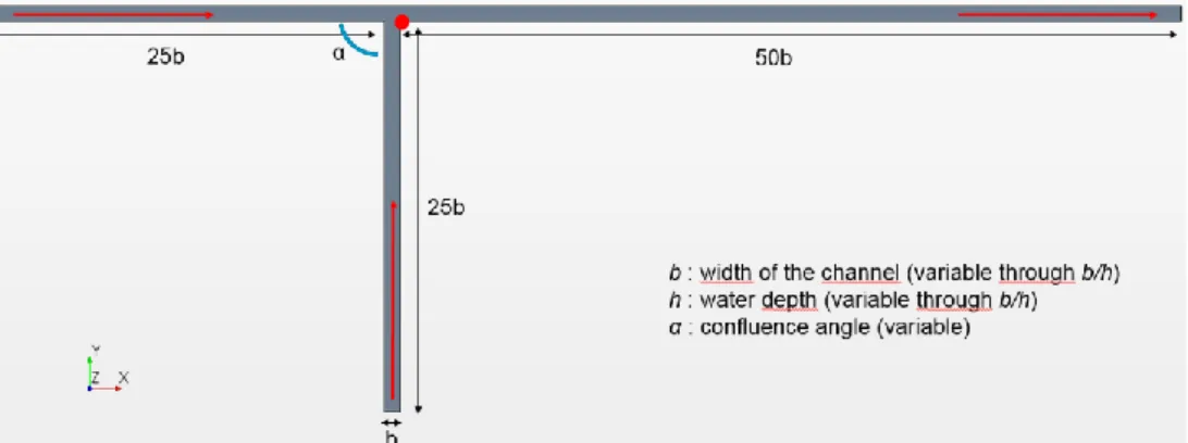
Here we consider ideal cases where the three branches of the confluence (upstream branch indicated u, lateral branch indicated l and downstream branch indicated d) have rectangular cross-sections with identical widths (b) and water depths (h). The simulated confluence is horizontal with plane, smooth and coincident beds. The confluence angle α between the two tributaries and the aspect ratio b/h, defined as the ratio between the width and the height of the cross-section, are thus the only two varying geometrical parameters considered for the study. The third tested parameter is the inflow momentum ratio, M*, defined as the ratio of the momentum of the tributary and of the main inflow. In our case, the momentum ratio M* is simply equal to the square of the volume flow rates ratio:
𝑀𝑀∗= 𝑚𝑚𝑙𝑙𝑢𝑢𝑙𝑙 𝑚𝑚𝑢𝑢𝑢𝑢𝑢𝑢= 𝜌𝜌𝑄𝑄𝑙𝑙∆𝑡𝑡×𝑢𝑢𝑙𝑙 𝜌𝜌𝑄𝑄𝑢𝑢∆𝑡𝑡×𝑢𝑢𝑢𝑢= 𝑢𝑢𝑙𝑙𝑢𝑢𝑙𝑙×𝑆𝑆 𝑢𝑢𝑢𝑢𝑢𝑢𝑢𝑢×𝑆𝑆= 𝑢𝑢𝑙𝑙2 𝑢𝑢𝑢𝑢2 = 𝑄𝑄𝑙𝑙2 𝑄𝑄𝑢𝑢2 (1)
The parametrical study consists in varying each one of these 3 parameters (b/h, α, M*) while keeping the other two constant, to analyse their individual role on the processes enhancing the mixing and to quantify their influence on the length for complete mixing Lm. In our study,
the confluence angle α varies from 30° to 90°; the aspect ratio b/h varies from 1 (typical of a sewer) to 50 (typical of very shallow flows, for example big rivers in Amazonia during the dry season); finally, the momentum ratio varies from 0.1 (very low tributary flow) to 9 (dominant tributary). Note that for each calculation the Reynolds and Froude numbers in the downstream branch are kept constant: Re=107 and Fr=0.1, to be representative of field scales.
Table 1. Values of the numerical parameters for 3D simulations on Star-CCM+ ©
Non-dimensional parameter Values interval Number of cases (values)
aspect ratio b/h [1; 50] 5 (1; 2.5; 5; 10; 50)
momentum ratio M* [0.111; 9] 5 (0.111; 0.25; 1; 4; 9)
confluence angle α [30°; 90°] 3 (30; 60; 90) total number : 75 calculations 2.2. Numerical model
The reference for the downstream axis is the downstream corner of the confluence, indicated with a red point on Fig.1. The distances are made non-dimensional using the width of the channel b, which is the same for all the branches of the confluence. The two inlets have a length of 25b and the downstream branch has a length of 50b, which permits to describe the mixing downstream of the confluence correctly.
The flow and mixing at the confluence are computed numerically using the commercial software of Computational Fluid Dynamics (CFD) Star-CCM+ ©, solving RANS equations coupled with the advection-diffusion equation. The turbulence model used is the Reynolds Stress Model (RSM). The passive scalar properties correspond to a chemical pollution: the molecular Schmidt number is high (666). The turbulent Schmidt number is fixed to 0.15, in agreement with previous comparisons in terms of dispersion with an experimental study with similar geometry at smaller scale by [13]. The mixing of the two inflows is analysed by setting the dimensionless concentration of passive scalar at 1 in one inflow and at 0 in the other.
Fig. 1. Geometry of the confluence for an angle of 90°. The flow direction is indicated with red arrows. As the Froude number is lower than 0.3, we use a rigid lid assumption [7] for the free surface. The boundary condition at the entrance of each branch is a fully-developed velocity profile obtained within a straight channel in another numerical simulation for the same discharge and geometry. The downstream boundary condition at the outlet is a hydrostatic pressure distribution.
The mesh is uniform for the whole domain of calculation, with cubic cells whose dimensions depend on the width of the channel b. The characteristic dimension of the basic cells is chosen to ensure two conditions: at least 10 cells along the vertical axis (of height h) and about 10 million cells (±20%) for the whole domain. The near-wall zones are meshed finer than the core of the domain, to ensure wall y+ values ranging between 50 and 100 and the flow at the wall is computed using a classical wall function.
3. Outputs
3.1. Definition of Lm
A classical criterion (called C1 in the sequel) to consider that the mixing is effectively
achieved is that the concentration variations within a cross-section are lower to ±5% of the downstream uniform concentration cm [12]. The strategy to obtain the length for complete
mixing Lm is then to count the number of cells whose concentration is out of the range
[0.95cm; 1.05cm], with cm the mean concentration in the downstream branch. This calculation
is performed at sections located at every channel width from 10b to 50b downstream of the confluence and every half-width from abscissa 0 to 10b. The spatial resolution for Lm thus
equals about 1b. Another available criterion (C2), to evaluate the length for perfect mixing
Lm is the calculation, for each cross-section defined previously, of the standard deviation of
the concentration in passive scalar [13]. The more the fluids are mixed, the lower is the standard deviation. In consequence, the standard deviation decreases when going downstream. We consider the complete mixing is achieved if C2<2%. Without loss of
generality, the length for perfect mixing Lm is localized in the following using the criterion
C2, which is independent from the final downstream concentration cm.
3.2. Quantification of secondary flows
To quantify the hydrodynamics influencing the mixing, especially the secondary currents, we calculate the intensity of secondary flow Is in a given cross-section of the downstream branch,
as defined by [14] for bend studies:
𝐼𝐼𝑠𝑠 =𝑅𝑅1 ℎ
2𝑈𝑈2∬ (𝑉𝑉2 𝑏𝑏 ℎ
0 0 + 𝑊𝑊2)𝑑𝑑𝑑𝑑𝑑𝑑𝑑𝑑 (2)
where Rh is the hydraulic radius of the cross-section, U the mean streamwise velocity, V and
W the local time-averaged transverse and vertical components of the velocity respectively. The higher the intensity of secondary flow is, the higher the transverse or vertical velocities are; thus Is represents the magnitude of the secondary flows.
4. Results
4.1. Flow description
Mixing in confluences is the result of hydrodynamic structures forming downstream of the confluence. The most effective flow structure for mixing appears to be the secondary currents in the downstream branch [1], see Fig.2. Under specific hydraulic conditions, it takes the form of a helical cell [1], which, near the confluence, promotes a macroscopic movement of the flow, strongly enhancing the mixing of the two inflows. The helical cell can be seen as the combination of the movement of the tributary flow toward the opposite bank near the free surface and then plugging along this bank, and the movement of the upstream flow to the tributary bank near the bottom and then going up along this bank. As the strength of this cell increases, the mixing efficiency also increases. However, due to viscous dissipation, this helical cell is only present close to the confluence and disappears more or less rapidly when moving downstream.
Fig. 2. Mean transverse velocity field (V and W components), with streamlines at x=b. The
lateral tributary comes from the left of the figure and the flow goes out the plan of the figure. The helical cell (centre) is preponderant for mixing. On the left, the low velocity zone is the recirculation zone. Case shown: angle α=90°, aspect ratio b/h=2.5 and momentum ratio M*=9
4.2. Impact of the confluence parameters on Lm and Is
The results show that Lm/b varies from about 10 to 200, depending on the confluence and
inflow characteristics. For the cases where the aspect ratio b/h=50, the length for complete mixing is too high (several hundred times the width of the channel) to be calculated with the method described before (the calculation domain would need to be extended). Thus, the results presented here are for aspect ratio b/h equal or lower than 10.
Fig.3 shows that for a large confluence angle (90°), the larger the momentum ratio M*, the shorter the length for complete mixing Lm, as long as the aspect ratio b/h is equal or lower
with M* (mostly for M*>1). The figure also shows the influence of the aspect ratio: as b/h increases, Lm/b increases. For shallower flows (b/h=10), the helical cell does not occupy the
whole cross-section, so the mixing is mainly due to transverse turbulent diffusion and the length for complete mixing strongly increases.
Fig. 3. Length for complete mixing with a confluence angle of 90°
For low confluence angles α, it is interesting to note that the maximum length for complete mixing Lm is reached for M*=1, whatever the aspect ratio. The shape of the curves in Fig.4
thus differs from those in Fig.3. Indeed, the helical cell is less strong as the angle is too low to initiate an important secondary flow for M*>1. Consequently, the mixing is mostly due to transverse turbulent diffusion only and so the length for complete mixing Lm is much higher
than for a larger confluence angle (Lm up to 200b).
Note that the lengths for complete mixing presented in figures 3 and 4 have been evaluated based on criterion C2; the use of criterion C1 leads to slightly longer Lm values, but the trends
are the same.
Fig. 4. Length for complete mixing with a confluence angle of 30°
0 50 100 150 200 0.1 1 10 Lm /b M* (LOG SCALE) b/h=1 b/h=2,5 b/h=5 b/h=10 0 50 100 150 200 0.1 1 10 Lm /b M* (LOG SCALE) b/h=1 b/h=2,5 b/h=5 b/h=10 6
with M* (mostly for M*>1). The figure also shows the influence of the aspect ratio: as b/h increases, Lm/b increases. For shallower flows (b/h=10), the helical cell does not occupy the
whole cross-section, so the mixing is mainly due to transverse turbulent diffusion and the length for complete mixing strongly increases.
Fig. 3. Length for complete mixing with a confluence angle of 90°
For low confluence angles α, it is interesting to note that the maximum length for complete mixing Lm is reached for M*=1, whatever the aspect ratio. The shape of the curves in Fig.4
thus differs from those in Fig.3. Indeed, the helical cell is less strong as the angle is too low to initiate an important secondary flow for M*>1. Consequently, the mixing is mostly due to transverse turbulent diffusion only and so the length for complete mixing Lm is much higher
than for a larger confluence angle (Lm up to 200b).
Note that the lengths for complete mixing presented in figures 3 and 4 have been evaluated based on criterion C2; the use of criterion C1 leads to slightly longer Lm values, but the trends
are the same.
0 50 100 150 200 0.1 1 10 Lm /b M* (LOG SCALE) b/h=1 b/h=2,5 b/h=5 b/h=10 0 50 100 150 200 0.1 1 10 Lm /b M* (LOG SCALE) b/h=1 b/h=2,5 b/h=5 b/h=10 4.3. Helical cell
For a given flow configuration, the intensity of secondary circulation Is reaches its maximum
at the cross-section where the magnitude of transverse and vertical velocities are maximum, i.e. where the intensity of the helical cell is also maximum. Fig. 5 shows that this cross-section is located a few channel widths downstream of the confluence (x/b~2). This indicator Is thus permits to follow the streamwise evolution of the helical cell strength.
Fig. 5. Intensity of secondary circulation (Is, left axis, closed symbols) and evolution of the standard
deviation of concentration in passive scalar (right axis, open symbols). Cases b/h=1, M*=9
From the figure 5, we observe the dominancy of secondary currents (higher Is values) in the first sections downstream of the confluence, whereas the mixing is controlled by transverse diffusion further from the confluence. Moreover, the influence of the angle of the confluence is very strong. Is decreases as the angle of the confluence decreases. Nevertheless, even for low angles (30°), a helical cell appears downstream of the confluence even if its intensity is much lower than for larger angles.
Fig.5 shows that the intensity of mixing (decrease of the standard deviation) is clearly linked to the secondary currents. Standard deviation decreases more rapidly in presence of strong secondary currents, and then decreases more gently when it is driven by transverse diffusion. As a result, the length for complete mixing in strongly influenced by the intensity of secondary circulation as depicted by the values for the cases shown above with the criterion C2 are shown in Table 2.
Table 2. Lm for cases b/h=1 and M*=9
Angle α 30° 60° 90°
Lm/b 38 20 9
The same analysis as Fig.5 but with M* instead of α (not shown here) leads to the following conclusion: Is increases with M*, whatever the angle or the aspect ratio. To conclude, we can
say that the intensity of the helical cell Is is directly linked to the transverse momentum
coming from the lateral tributary: Is increases as the discharge (so also M*) or the angle
increases. 0 0.05 0.1 0.15 0.2 0.25 0.3 0.35 0.4 0.45 0.5 0 0.005 0.01 0.015 0.02 0.025 0.03 0 2 4 6 8 10 C2 Is x/b 30° Is 60° Is 90° Is 30° C2 60° C2 90° C2 C2 criterion
5. Conclusion
The study has shown that mixing in confluences strongly depends on the hydrodynamic and geometric parameters of the inflows. Numerical simulations are able to fairly compute the hydrodynamics and the passive scalar mixing in complex flows such as confluences; it permits to multiply the number of cases and thus to set a parametric study of passive scalar mixing in confluences. Secondary flows developing downstream of the confluence have a helical shape that intermingles the two upstream flows. The intensity of this helical cell is directly linked to the length for complete mixing Lm, which varies from 10b to more than
200b, depending on the parameters of the confluence. The aspect ratio is the considered parameter which has the more impact of the length for complete mixing. A major result is that for a low angle of confluence, which is the most common case in the nature, with inflows of equal width and depth, the length for complete mixing is maximum when the two inflows have the same discharge.
Sébastien Pouchoulin held a doctoral fellowship from la Région Auvergne Rhône Alpes. The study was supported by OTHU (Oberservatoire de Terrain en Hydrologie Urbaine).
References
1. A. Shakibainia, M. R. M. Tabatabai, A. R. Zarrati, Can. J. Civ. Eng. 37: 772-781 (2010) 2. M. Launay, J. Le Coz, B. Camenen, C. Walter, H. Angot, G. Dramais, J-B. Faure, M.
Coquery, J. Hydro-environment Research 9,1,120-132 (2015) 3. M. Launay, PhD thesis (2014)
4. S.N. Lane, D.R. Parsons, J.L. Best, O. Orfeo, R.A. Kostaschuk, R.J. Hardy, J. Geophy. Research, vol.113 (2008)
5. P.M. Biron, A.S. Ramamurthy, F. Asce, S. Han, J. Hydraul. Eng. 130(3): 243-253 (2004) 6. K.F. Bradbrook, S.N. Lane, K.S. Richards, Am. Geophy. U. 36,9 : 2731-2746 (2000) 7. L. Schindfessel, S. Creelle, T. De Mulder, Water 7,4724-4751 (2015)
8. L.J. Weber, E. D. Schumate, N. Mawer, J. Hydraul. Eng., 127(5), 340-350 (2001) 9. E. Mignot, H. Bonakdari, P. Knothe, G. Lipeme-Kouyi, A. Bessette, N. Rivière, J-L.
Bertrand-Krajewski, Water Sci. Tech., 66(6),132-1332 (2012)
10. B.L. Rhoads, S.T. Kenworthy, Geomorphology, 11(4), 273-293 (1995) 11. C. Gualtieri, A. Angeloudis, F. Bombardelli, S. Jha, T. Stoesser, Fluids (2017)
12. H. B. Fischer, E. J. List, R. C. Y. Koh, J. Imberger, N. H. Brooks, Academic Press (1979) 13. A. Dalmon, E. Mignot, N. Rivière, G. Lipeme-Kouyi, A. Momplot, C. Gonzalez, C.
Escauriaza, Congrès Français de Mécanique (2015)
14. K. Sudo, M. Sumida, H. Hibara, Exp. Fluids 30,246-252 (2001)