HAL Id: insu-02426287
https://hal-insu.archives-ouvertes.fr/insu-02426287
Submitted on 10 Jul 2020
HAL is a multi-disciplinary open access
archive for the deposit and dissemination of
sci-entific research documents, whether they are
pub-lished or not. The documents may come from
teaching and research institutions in France or
abroad, or from public or private research centers.
L’archive ouverte pluridisciplinaire HAL, est
destinée au dépôt et à la diffusion de documents
scientifiques de niveau recherche, publiés ou non,
émanant des établissements d’enseignement et de
recherche français ou étrangers, des laboratoires
publics ou privés.
records with ground-based DOAS networks: the role of
measurement and comparison uncertainties
Steven Compernolle, Tiji Verhoelst, Gaia Pinardi, Jose Granville, Daan
Hubert, Arno Keppens, Sander Niemeijer, Bruno Rino, Alkis Bais, Steffen
Beirle, et al.
To cite this version:
Steven Compernolle, Tiji Verhoelst, Gaia Pinardi, Jose Granville, Daan Hubert, et al.. Validation of
Aura-OMI QA4ECV NO2 climate data records with ground-based DOAS networks: the role of
mea-surement and comparison uncertainties. Atmospheric Chemistry and Physics, European Geosciences
Union, 2020, 20 (13), pp.8017-8045. �10.5194/acp-20-8017-2020�. �insu-02426287�
https://doi.org/10.5194/acp-20-8017-2020 © Author(s) 2020. This work is distributed under the Creative Commons Attribution 4.0 License.
Validation of Aura-OMI QA4ECV NO
2
climate data records with
ground-based DOAS networks: the role of measurement and
comparison uncertainties
Steven Compernolle1, Tijl Verhoelst1, Gaia Pinardi1, José Granville1, Daan Hubert1, Arno Keppens1,
Sander Niemeijer2, Bruno Rino2, Alkis Bais3, Steffen Beirle4, Folkert Boersma5,8, John P. Burrows6,
Isabelle De Smedt1, Henk Eskes5, Florence Goutail7, François Hendrick1, Alba Lorente8, Andrea Pazmino7,
Ankie Piters5, Enno Peters6, Jean-Pierre Pommereau7, Julia Remmers4, Andreas Richter6, Jos van Geffen5,
Michel Van Roozendael1, Thomas Wagner4, and Jean-Christopher Lambert1
1Royal Belgian Institute for Space Aeronomy (BIRA-IASB), Uccle, Belgium
2s[&]t Corporation, Delft, the Netherlands
3Aristotle University of Thessaloniki, Laboratory of Atmospheric Physics (AUTH), Thessaloniki, Greece
4Max Planck Institute for Chemistry (MPIC), Mainz, Germany
5Royal Netherlands Meteorological Institute (KNMI), De Bilt, the Netherlands
6Institute of Environmental Physics, University of Bremen (IUP-B), Bremen, Germany
7Laboratoire Atmosphères, Milieux, Observations Spatiales, CNRS, Guyancourt, France
8Wageningen University, Meteorology and Air Quality Group, Wageningen, the Netherlands
Correspondence: Steven Compernolle ([email protected]) Received: 27 September 2019 – Discussion started: 2 January 2020
Revised: 30 April 2020 – Accepted: 24 May 2020 – Published: 10 July 2020
Abstract. The QA4ECV (Quality Assurance for Essential Climate Variables) version 1.1 stratospheric and tropospheric
NO2 vertical column density (VCD) climate data records
(CDRs) from the OMI (Ozone Monitoring Instrument) satel-lite sensor are validated using NDACC (Network for the Detection of Atmospheric Composition Change) zenith-scattered light differential optical absorption spectroscopy (ZSL-DOAS) and multi-axis DOAS (MAX-DOAS) data as a reference. The QA4ECV OMI stratospheric VCDs have
a small bias of ∼ 0.2 Pmolec. cm−2 (5 %–10 %) and a
dis-persion of 0.2 to 1 Pmolec. cm−2 with respect to the
ZSL-DOAS measurements. QA4ECV tropospheric VCD obser-vations from OMI are restricted to near-cloud-free scenes, leading to a negative sampling bias (with respect to the unrestricted scene ensemble) of a few peta molecules per
square centimetre (Pmolec. cm−2) up to −10 Pmolec. cm−2
(−40 %) in one extreme high-pollution case. The QA4ECV OMI tropospheric VCD has a negative bias with respect to
the MAX-DOAS data (−1 to −4 Pmolec. cm−2), which is
a feature also found for the OMI OMNO2 standard data
product. The tropospheric VCD discrepancies between satel-lite measurements and ground-based data greatly exceed the combined measurement uncertainties. Depending on the site, part of the discrepancy can be attributed to a combination of comparison errors (notably horizontal smoothing differ-ence error), measurement/retrieval errors related to clouds and aerosols, and the difference in vertical smoothing and a priori profile assumptions.
1 Introduction
Nitrogen oxides (NOx=NO2+NO) play a significant role
in the atmosphere, as they catalyse tropospheric ozone for-mation via a suite of chemical reactions, impact the oxidiz-ing capacity of the atmosphere and, thus, influence the atmo-spheric burdens of major pollutants like methane and carbon monoxide (Seinfeld and Pandis, 1997). In addition, they are responsible for secondary aerosol formation (Sillman et al., 1990). Fossil fuel combustion is the dominant source of the
global NOx emission budget (∼ 50 %), followed by
natu-ral emissions from soils, lightning and open vegetation fires
(Delmas et al., 1997). High ozone, aerosol and NOx have
adverse effects on human health (Hoek et al., 2013; World Health Organization, 2013), and the recommended limits from the European Union (EU) and the World Health Or-ganization (WHO) are often exceeded, especially in densely populated and industrialized regions (European Environment
Agency, 2018). Therefore, emissions of NOx have been the
main target of abatement strategies worldwide (e.g. the
Pro-tocol of Gothenburg, 1999). The effects of NOxemissions on
climate are complex and are currently not fully understood.
On the one hand, emissions of NOx result in an increase in
ozone and, thus, a net warming (as ozone is a greenhouse gas); on the other hand, they lead to a decrease in methane abundances at longer timescales and, therefore, to a cooling effect (Myhre et al., 2013). Due to their indirect impact on radiative forcing and potential affect on climate (Shindell
et al., 2009), NOx has been identified as an “Essential
Cli-mate Variable” (ECV) precursor by the Global CliCli-mate
Ob-serving System (GCOS; GCOS, 2016). NOx is also present
in the stratosphere (Noxon, 1979), where it contributes to the catalytic destruction of ozone (Crutzen, 1970).
Observations from satellite nadir-viewing sensors are
es-sential for mapping the global multiyear picture of the NOx
distribution and trend. However, the quality of these data sets needs to be carefully assessed using ground-based measure-ments at different sites (see e.g. Petritoli et al., 2004; Pinardi et al., 2014; Heue et al., 2005; Brinksma et al., 2008; Celar-ier et al., 2008, for validations on GOME, Global Ozone Monitoring Experiment; GOME-2, Global Ozone Monitor-ing Experiment-2; SCIAMACHY, ScannMonitor-ing ImagMonitor-ing Ab-sorption Spectrometer for Atmospheric Chartography; and OMI, Ozone Monitoring Instrument data). A limitation often encountered is that uncertainties in satellite and/or based data are not adequately characterized, and the ground-based data sets are generally not harmonized across net-works.
The EU Seventh Framework Programme (FP7) QA4ECV (Quality Assurance for Essential Climate Variables) project (http://www.qa4ecv.eu, last access: 20 April 2020) demon-strated how reliable and traceable quality information can be provided for satellite and ground-based measurements of cli-mate and air quality parameters. Here, we highlight three of its achievements:
1. The development of a quality assurance framework for climate data records (CDRs; Nightingale et al., 2018), covering aspects such as product traceability, uncer-tainty description, validation and documentation, fol-lowing international standards (QA4EO, 2019; Joint Committee for Guides in Metrology, 2008, 2012). Among its components are a generic validation protocol (Compernolle et al., 2018, building upon Keppens et al., 2015), a compilation of recommended terminology for
CDR quality assessment (Compernolle and Lambert, 2017; Compernolle et al., 2018) and a validation server (Compernolle et al., 2016; Rino et al., 2017); the lat-ter is a prototype for the operational validation servers for S5P-MPC (Sentinel-5P Mission Performance Cen-ter) and CAMS (Copernicus Atmosphere Monitoring Service).
2. The establishment of multi-decadal CDRs for six ECVs following the guidelines of the quality assurance
frame-work; among them are the QA4ECV NO2 (Lorente
et al., 2017; Zara et al., 2018; Boersma et al., 2018) and the HCHO (De Smedt et al., 2018) version 1.1 satellite products, which are available for several sensors.
3. The development of an NO2 and HCHO long-term
ground-based data set for 10 MAX-DOAS instruments, harmonized with respect to measurement protocol and data format and with an extensive uncertainty charac-terization (Hendrick et al., 2016; Richter et al., 2016). A general across-community issue in the geophysical valida-tion of satellite data sets with respect to ground-based refer-ence measurements is the additional uncertainty that appears when comparing data sets characterized by different tempo-ral/spatial/vertical sampling and smoothing properties (Loew et al., 2017). This is especially critical for short-lived tropo-spheric gases (Richter et al., 2013b). This issue was the focus of the EU Horizon 2020 GAIA-CLIM (Gap Analysis for In-tegrated Atmospheric ECV CLImate Monitoring; Verhoelst et al., 2015; Verhoelst and Lambert, 2016) project.
In this work, we report a comprehensive validation of
the QA4ECV NO2 version 1.1 data product on the OMI
sensor using the ground-based measurements acquired by DOAS (differential optical absorption spectroscopy) UV–Vis instrument networks developed in the context of the Net-work for the Detection of Atmospheric Composition Change (NDACC) as a reference. Zenith-scattered light DOAS (ZSL-DOAS) data obtained routinely as part of NDACC moni-toring activities are used to validate the stratospheric verti-cal column density (VCD), while multi-axis DOAS (MAX-DOAS) data, either from NDACC or further harmonized within the QA4ECV project, are used to validate the
tropo-spheric VCD. We focus on how well the ex ante1
uncertain-ties and comparison errors explain the observed discrepan-cies, making use of the framework and methodology devel-oped within the QA4ECV and GAIA-CLIM projects.
This paper is structured as follows. In Sect. 2, the satellite and reference data sets are described. Section 3.1 provides details about the validation methodology. In Sect. 3.2, we
outline how the quality screening of QA4ECV OMI NO2,
1An ex ante quantity does not rely on a statistical comparison
with external data (von Clarmann, 2006). This is to be contrasted with ex post quantities like the mean difference of satellite data vs. reference data.
notably the exclusion of cloudy scenes, leads to
underesti-mated early afternoon tropospheric NO2VCDs. Section 3.3
presents the comparison of the QA4ECV OMI stratospheric
NO2 VCD with ZSL-DOAS. In Sect. 3.4, the satellite
tro-pospheric VCD is compared with measurements from 10 MAX-DOAS instruments. The differences are analysed in relation to the uncertainties and the comparison errors. Po-tential causes of the discrepancies (e.g. horizontal smooth-ing difference error, low-lysmooth-ing clouds or aerosols, and profile shape uncertainty) and attempts to resolve the discrepancies are then discussed. Finally, the conclusions are formulated in Sect. 4.
2 Description of the data sets
2.1 Satellite data
2.1.1 QA4ECV OMI NO2
The QA4ECV NO2 OMI version 1.1 data product is
re-trieved from Level 1 UV–Vis spectral measurements (OMI-Aura_L1-OML1BRVG radiance files) from the Dutch– Finnish UV–Vis nadir-viewing OMI (Ozone Monitoring In-strument) spectrometer on NASA’s Earth Observing System Aura (EOS-Aura) polar satellite. The nominal footprint of
the OMI ground pixels is 24 × 13 km2(across × along track)
at nadir to 165 × 13 km2at the edges of the 2600 km swath,
and the ascending node local time is 13:42 LT. For more de-tails on the instrument, see Levelt et al. (2006). The data product provides a Level 2 (L2) tropospheric, stratospheric
and total NO2VCD.
The QA4ECV algorithm includes the following steps:
(i) retrieving the total slant column density (SCD) Ns using
differential optical absorption spectroscopy (DOAS), (ii)
es-timating the stratospheric SCD Ns,stratfrom data assimilation
using the TM5 (Tracer Model, version 5) chemistry trans-port model (CTM), (iii) obtaining the tropospheric contribu-tion by subtraccontribu-tion and (iv) calculating the tropospheric air
mass factors (AMFs) Mtropby converting the SCD to a VCD
Nv,trop(see Table 1). The retrieval equation is as follows:
Nv,trop=
Ns−Ns,strat
Mtrop
(1) More information can be found in the “Product Specification
Document for the QA4ECV NO2ECV precursor product”
(Boersma et al., 2017b) and in Zara et al. (2018) and Boersma et al. (2018). A preliminary evaluation of the data indicated
that QA4ECV NO2values are 5 %–20 % lower than the
ear-lier version of the OMI NO2 data product, DOMINO v2,
over polluted regions, and that they agree slightly better with
MAX-DOAS NO2 VCD measurements in Tai’an (China)
and De Bilt (the Netherlands) than the DOMINO v2 VCDs (Lorente et al., 2017; Lorente Delgado, 2019).
The data product files contain a comprehensive amount of metadata. For each pixel, the satellite data product
pro-vides a total ex ante uncertainty on the retrieved tropospheric
VCD as well as a breakdown of the uncertainty uSAT into
an ex ante uncertainty budget with the following uncertainty
source components: uncertainty in total SCD uSAT,Ns;
strato-spheric SCD uSAT,Ns,strat; and tropospheric AMF uSAT,Mtrop,
which contains contributions from uncertainties in surface
albedo uSAT,As, cloud fraction (CF) uSAT,fcl, cloud pressure
uSAT,pcl and a priori profile shape uSAT,Sa; and an
albedo-CF cross-term, with cAs,fcl representing the error correlation
coefficient between both properties (Boersma et al., 2018, Sect. 6).
u2SAT=u2SAT,Ns+u2SAT,Ns,strat+u2SAT,Mtrop u2SAT,M trop=u 2 SAT,As+u 2 SAT,fcl+u 2 SAT,pcl+u 2 SAT,Sa +2cAs,fcluSAT,AsuSAT,fcl (2)
Furthermore, the satellite data files provide several relevant instrument parameters, influence quantities (e.g. cloud frac-tion, surface albedo and terrain height), intermediate quanti-ties (e.g. SCD, AMF and stratospheric SCD) and the column
averaging kernel aSAT, which relates the retrieved VCD to the
true profile. The a priori NO2profiles (simulated with TM5)
are not stored in the data files. If users have to adapt a
(mea-sured or modelled) profile xhat a high vertical resolution to
the vertical sensitivity of the satellite, they can apply Eq. (11) from Eskes and Boersma (2003):
aSAT·xh=xh,sm, (3)
where the a priori profile xSAT,a is not explicit. The
depen-dence of the retrieval on xSAT,a is already implicit via the
averaging kernel aSAT.
However, the reference data in the current work are col-umn retrievals or profile retrievals with a limited vertical res-olution and are based on an a priori profile that is different from the satellite retrieval. Before smoothing, satellite and reference retrievals should be adjusted such that they use the same a priori profile (Rodgers and Connor, 2003); therefore, knowledge of the satellite a priori profile is relevant. These can be derived from the TM5-MP data files (Huijnen et al., 2010; Williams et al., 2017), which are available upon re-quest (see Boersma et al., 2017b, for contact details), by spa-tially interpolating the profiles to the location of the satellite ground pixel.
In this work, we considered data from 2004 up to and in-cluding 2016 for the tropospheric VCD and up to and includ-ing 2017 for the stratospheric VCD.
2.1.2 OMI STREAM stratospheric NO2
The Stratospheric Estimation Algorithm From Mainz (STREAM; Beirle et al., 2016) was included as an alternative
stratospheric estimation scheme in the QA4ECV NO2data
files. In STREAM, the estimate of stratospheric columns is based on satellite observations with a negligible tropospheric
contribution, i.e. generally over regions with low
tropo-spheric NO2levels, and for satellite pixels with high clouds,
where the tropospheric column is shielded. The stratospheric field is then smoothed and interpolated globally, assuming
that the spatial pattern of stratospheric NO2does not feature
strong gradients.
2.1.3 NASA OMNO2 data product
Although not the main focus of this work, we do include
NASA’s OMI NO2 data – OMNO2 version 3.1 (Bucsela
et al., 2016; Krotkov et al., 2017) – as a benchmark com-parison of an alternative retrieval product with QA4ECV
MAX-DOAS. Like QA4ECV OMI NO2, OMNO2 is also
based on the DOAS approach, although nearly all retrieval steps are different between the QA4ECV and NASA OMI
NO2 algorithms (Table 1). A detailed comparison of the
QA4ECV and NASA fitting approaches showed small
dif-ferences between NO2SCDs (Zara et al., 2018); thus,
differ-ences between the spectral fitting approaches only explain a small part of the differences in the tropospheric VCDs. The stratospheric correction approach differs between the two al-gorithms. Although the QA4ECV and NASA stratospheric SCDs have not been compared directly, previous evalua-tions suggest that differences between the approaches typi-cally lead to small but spatially widespread differences of up
to 0.5–1.0 × 10¹⁵molec. cm−2 in tropospheric VCDs. This
leaves differences between the tropospheric AMF calcula-tions (and especially the prior information used in their cal-culations) as the most likely explanation for the lower NASA
values compared with QA4ECV NO2VCDs (e.g. Goldberg
et al., 2017).
2.2 Ground-based data
2.2.1 Zenith-scattered light DOAS
The ZSL-DOAS data are part of the Network for the Detection of Atmospheric Composition Change (NDACC; De Mazière et al., 2018, see also http://www.ndaccdemo. org/, last access: 22 April 2020), which is a major contributor to the WMO’s Global Atmospheric Watch. A significant part of the multi-decadal ZSL-DOAS data is provided by the Sys-tème d’Analyse par Observation Zénithale (SAOZ; see Pom-mereau and Goutail, 1988) subnetwork from the IPSL At-mospheres Laboratory (LATMOS), using SAOZ instrumen-tation in automated data acquisition mode and with fast data delivery.
Zenith-sky measurements are performed during twilight at sunrise and sunset. Due to this measurement geometry with a long optical path in the stratosphere, the measured
col-umn is about 14 times more sensitive to stratospheric NO2
than to tropospheric NO2(Solomon et al., 1987). Moreover,
it allows for usable measurements to also be made during cloudy conditions. Processing followed the NDACC standard
operation procedure (http://ndacc-uvvis-wg.aeronomie.be/ tools/NDACC_UVVIS-WG_NO2settings_v4.pdf, last ac-cess: 22 April 2020), as implemented, for instance, in the LATMOS_v3 SAOZ processing. From slant column inter-comparisons, Vandaele et al. (2005) deduce an uncertainty of about 4 %–7 %, but this excludes the uncertainty on the AMF required to convert the slant to vertical columns. Ionov et al. (2008) estimate a total uncertainty on the vertical columns of 21 %, but this is probably an overestimation for the most recent processing, as Bognar et al. (2019) now suggest a 13 % total uncertainty. A visualization of the geographical distribution of the instruments is provided in Fig. 1. More details about the particular co-location scheme, considering the large horizontal smoothing of these measurements and the photochemical adjustment required to convert twilight measurements to satellite overpass times, are provided in Sect. 3.1.
2.2.2 Multi-axis DOAS
The tropospheric NO2VCD data used as a reference are a
long-term record of MAX-DOAS (multi-axis DOAS) mea-surements from 10 instruments, reprocessed by different teams for the QA4ECV project (see Table 2). MAX-DOAS instruments measure scattered sunlight under different view-ing elevations from the horizon to the zenith (Platt and Stutz, 2008). The observed light travels a long path (the length is dependent on the elevation angle) in the lower tropo-sphere, while the stratospheric contribution is removed by a reference zenith measurement. Two different MAX-DOAS data processing methods were used for the current validation study, QA4ECV MAX-DOAS and bePRO (Belgian Profil-ing) MAX-DOAS (Clémer et al., 2010), with the latter being part of NDACC.
Thanks to an extensive harmonization effort within
the QA4ECV project, reference QA4ECV
MAX-DOAS data sets were produced by the different teams for all 10 instruments. These data sets are available
at http://uv-vis.aeronomie.be/groundbased/QA4ECV_
MAXDOAS/index.php (last access: 22 April 2020).
This effort was based on a four-step approach (see http://uv-vis.aeronomie.be/groundbased/QA4ECV_
MAXDOAS/QA4ECV_MAXDOAS_readme_website.pdf, last access: 22 April 2020; Hendrick et al., 2016; Richter et al., 2016; Peters et al., 2017), including (i) the establish-ment of recommendations for DOAS analysis settings from
an intercomparison of NO2slant column densities retrieved
from common spectra, (ii) the development of NO2 AMF
look-up tables (LUTs) to harmonize the conversion of SCDs into VCDs, (iii) the establishment of a first harmonized error budget and (iv) the generation of MAX-DOAS data files in the Generic Earth Observation Metadata Standard (GEOMS) as a common format. It is worth noting that as only SCDs measured at a relatively high elevation angle
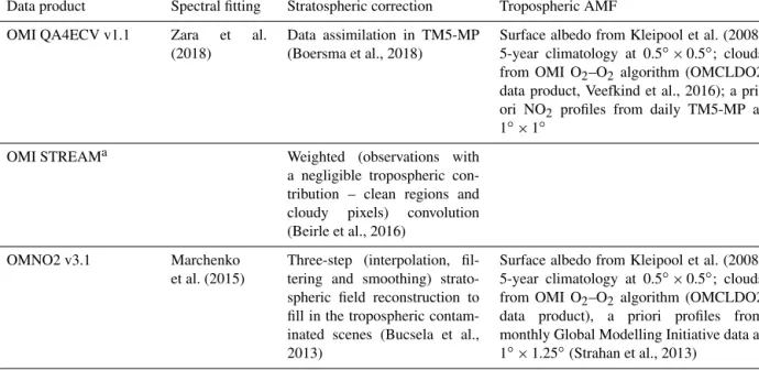
Table 1. The OMI satellite data products considered in this work.
Data product Spectral fitting Stratospheric correction Tropospheric AMF OMI QA4ECV v1.1 Zara et al.
(2018)
Data assimilation in TM5-MP (Boersma et al., 2018)
Surface albedo from Kleipool et al. (2008) 5-year climatology at 0.5◦×0.5◦; clouds from OMI O2–O2 algorithm (OMCLDO2
data product, Veefkind et al., 2016); a pri-ori NO2 profiles from daily TM5-MP at 1◦×1◦
OMI STREAMa Weighted (observations with a negligible tropospheric con-tribution – clean regions and cloudy pixels) convolution (Beirle et al., 2016)
OMNO2 v3.1 Marchenko et al. (2015)
Three-step (interpolation, fil-tering and smoothing) strato-spheric field reconstruction to fill in the tropospheric contam-inated scenes (Bucsela et al., 2013)
Surface albedo from Kleipool et al. (2008) 5-year climatology at 0.5◦×0.5◦; clouds from OMI O2–O2 algorithm (OMCLDO2
data product), a priori profiles from monthly Global Modelling Initiative data at 1◦×1.25◦(Strahan et al., 2013)
aOMI STREAM stratospheric VCD is contained in the OMI QA4ECV v1.1 data files.
Figure 1. Global distribution of the ZSL-DOAS instruments used in this study. Red markers indicate SAOZ instruments, and blue markers indicate other NDACC ZSL-DOAS instruments.
and a priori profile shape on the retrieval in this QA4ECV approach, the horizontal location of the centre of the effec-tively probed air mass is close to the instrument location
(typically within 1 km). The NO2AMF LUTs are produced
using the bePRO/LIDORT radiative transfer suite (Clémer et al., 2010; Spurr, 2008). This tool uses the following
input (among others): a set of NO2 vertical profile shapes,
vertical averaging kernel LUTs, geometry parameters (e.g. solar angles and viewing angles) and aerosol optical density (AOD) vertical profile shapes. Column averaging kernel LUTs were calculated based on the Eskes and Boersma (2003) approach, using the bePRO/LIDORT radiative trans-fer model initialized with similar parameter values to those used for the calculation of the AMF LUTs. Interpolated
AMFs as well as the corresponding vertical profile shapes and column averaging kernels are generated by the tool. More detail is provided in Hendrick et al. (2016).
The second processing method, bePRO MAX-DOAS (Clémer et al., 2010; Hendrick et al., 2014; Vlemmix et al., 2015), is available for three BIRA-IASB instruments (at Bujumbura, Uccle and Xianghe). This approach, which is based on the optimal estimation method (OEM; see Rodgers, 2000), provides profile measurements, albeit with a limited degree of freedom for signal in the vertical dimension, which is typically ∼ 2 (Bujumbura and Uccle) or ∼ 3 (Xianghe). The horizontal extension of the air masses probed by profile retrieval MAX-DOAS is about 5–15 km from the instrument in the viewing direction (Richter et al., 2013a). The exten-sion depends on the atmospheric visibility (lower extenexten-sion
for lower visibility) and the altitude of the NO2layer (lower
extension with decreasing profile height). This is in line with the typical distances estimated by studies such as Irie et al. (2011, their Fig. 17). The horizontally projected area of the air mass probed by the MAX-DOAS is estimated to be of
the order of 0.01 to 0.2 km2for QA4ECV MAX-DOAS and
∼1 km2 for bePRO MAX-DOAS, assuming a 1◦ field of
view and a simple geometrical approximation.
There is a clear distinction between the QA4ECV MAX-DOAS and bePRO retrieval algorithms. In the QA4ECV MAX-DOAS algorithm, the VCD is obtained by dividing a differential SCD by a differential AMF at a single elevation angle (see Sect. 1.3 of Hendrick et al., 2016). In the bePRO approach (Clémer et al., 2010; Hendrick et al., 2014; Vlem-mix et al., 2015), a VCD is obtained by integrating a vertical
NO2profile retrieved by an optimal estimation method using
measurements at several elevation angles.
MAX-DOAS instruments probe the lower troposphere, with the highest sensitivity (described by the column averag-ing kernel) close to the surface, typically in the lowest 1.5 km of the atmosphere. Nevertheless, the vertical grid extends to
∼10 km for QA4ECV MAX-DOAS and ∼ 3 km for bePRO
MAX-DOAS.
The MAX-DOAS sites span a wide range of NO2
levels, from relatively low at Observatoire de Haute-Provence (OHP) and Bujumbura, with a mean tropospheric MAX-DOAS VCD around the OMI overpass time of ∼
3 Pmolec. cm−2, to strongly polluted at Xianghe, with a mean
MAX-DOAS value of ∼ 24 Pmolec. cm−2(see Fig. 3c, black
boxplots), whereas the other sites are moderately polluted
(mean value of between 5.6 and 11 Pmolec. cm−2).
The MAX-DOAS tropospheric VCD is provided with an ex ante uncertainty in the GEOMS data files. Unfortunately the uncertainty estimation approach employed is not harmo-nized among all data providers. Therefore, we set the total uncertainty at 22.2 % of the retrieved VCD for QA4ECV MAX-DOAS instead, following the QA4ECV deliverable D3.9 recommendation (Richter et al., 2016). Using
sensitiv-ity tests, aerosol effects (20 %) and the NO2a priori profile
shape (8 %) were identified as the main contributors to the
MAX-DOAS uncertainty, whereas the uncorrelated instru-ment noise was only 2 %. However, we did not follow D3.9 (Richter et al., 2016) in its recommended division of the un-certainty into the random error and systematic error
contri-butions2and consider only a total uncertainty. Regarding
be-PRO MAX-DOAS, we consider a 12 % total uncertainty for Uccle and Xianghe (following Hendrick et al., 2014), and a 21 % total uncertainty for Bujumbura (following Gielen et al., 2017). We finally note that an absolute scale uncer-tainty estimate might be more appropriate for clean sites.
We note that the bePRO profile retrieval algorithm has re-cently been compared to several other retrieval algorithms (Frieß et al., 2019; Tirpitz et al., 2020). In future validation work, the consideration of other retrieval algorithms that per-formed well in the intercomparison exercises of Frieß et al. (2019) and Tirpitz et al. (2020) would be of high interest.
As the accuracy of satellite or ground-based remote sens-ing can be affected by the presence of aerosol, tracksens-ing aerosol optical depth (AOD) is useful. The bePRO MAX-DOAS provides AOD measurements at the same
tempo-ral sampling resolution as the NO2 measurements. The
QA4ECV MAX-DOAS provides an AOD climatology (Hen-drick et al., 2016) based on AERONET (Aerosol Robotic Network) data (Giles et al., 2019); however, we found that the precision of this climatological data set was inadequate for the current work, especially for urban sites. Instead, we considered AOD directly from AERONET (Giles et al., 2019; http://aeronet.gsfc.nasa.gov, last access: 22 Septem-ber 2019), whose measurements are based on Cimel Elec-tronique Sun–sky radiometers. Level 2.0 AOD at a wave-length of 440 nm was chosen, which is within the QA4ECV MAX-DOAS retrieval window of 425–490 nm. Note that the AERONET data are already cloud filtered.
A limitation when investigating AOD dependencies in satellite MAX-DOAS comparisons using AERONET AOD
with QA4ECV MAX-DOAS tropospheric NO2 VCD data
(compared with using bePRO AOD with bePRO NO2data)
is that it implies subsetting: for part of the QA4ECV
MAX-DOAS NO2 data, no co-located AERONET AOD
data are available. Moreover, as opposed to the bePRO
2In D3.9, the systematic error uncertainty is set at 3 %, arising
from absorption cross-section-related systematic error uncertainty on the SCD, whereas the random error uncertainty is set at 22 %, arising from uncertainty on the AMF. However, the assumption that an error in a priori profile shape, for example, would translate to a random error on the retrieved column is not evident in our opinion. In a later analysis (Hendrick et al., 2018), a comparison of QA4ECV MAX-DOAS with more advanced MAX-DOAS profiling methods was performed. This highlighted systematic differences between −12 % and +7 %, which are considerably larger than the system-atic error uncertainty of 3 % recommended by the D3.9. This sug-gests that a larger part of the total uncertainty is due to systematic error. Therefore, in this work, we only consider a total uncertainty of 22.2 %, which is derived from the sum of the recommended sys-tematic and random components in quadrature.
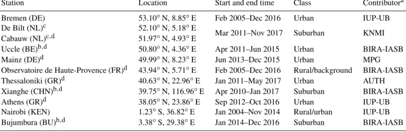
Table 2. Overview of contributing sources for the QA4ECV MAX-DOAS reference data set.
Station Location Start and end time Class Contributora Bremen (DE) 53.10◦N, 8.85◦E Feb 2005–Dec 2016 Urban IUP-UB De Bilt (NL)c 52.10◦N, 5.18◦E
Mar 2011–Nov 2017 Suburban KNMI Cabauw (NL)c,d 51.97◦N, 4.93◦E
Uccle (BE)b,d 50.80◦N, 4.36◦E Apr 2011–Jun 2015 Urban BIRA-IASB Mainz (DE)d 49.99◦N, 8.23◦E Jun 2013–Dec 2015 Urban MPG Observatoire de Haute-Provence (FR)d 43.94◦N, 5.71◦E Feb 2005–Dec 2016 Rural/background BIRA-IASB Thessaloniki (GR)d 40.63◦N, 22.96◦E Jan 2011–May 2017 Urban AUTH Xianghe (CHN)b,d 39.75◦N, 116.96◦E Apr 2010–Jan 2017 Suburban BIRA-IASB Athens (GR)d 38.05◦N, 23.86◦E Sep 2012–Oct 2016 Urban IUP-UB Nairobi (KEN) 1.23◦S, 36.82◦E Jan 2004–Nov 2014 Rural/urban IUP-UB Bujumbura (BU)b,d 3.38◦S, 29.38◦E Jan 2014–Dec 2016 Suburban BIRA-IASB
aContributing teams: the Aristotle University of Thessaloniki (AUTH), the Royal Belgian Institute of Space Aeronomy (BIRA-IASB), the Institute of
Environmental Physics at the University of Bremen (IUP-UB), the Max Planck Institute (MPG) and the Royal Netherlands Meteorological Institute (KNMI).bFor this sensor, bePRO MAX-DOAS data (providing profile data) are also available.cThe same instrument was operated at two different locations, De Bilt and Cabauw, which are approximately 30 km apart.dAn AERONET instrument, measuring aerosol optical depth, is located at this site or in close proximity.
NO2/bePRO AOD combination, co-located QA4ECV
MAX-DOAS NO2/AERONET AOD data pairs have a
tem-poral co-location mismatch and (where instruments are at different locations) a spatial co-location mismatch. A test was performed (results not shown) using the bePRO
NO2/AERONET AOD combination, and it was generally
found that the results are less clear than for the bePRO
NO2/bePRO AOD combination.
3 Validation
3.1 Validation methodology
The generic validation protocol is similar to that outlined by Keppens et al. (2015), and it is tailored within the QA4ECV
project for the ECVs NO2, HCHO and CO (Compernolle
et al., 2018). Terms and definitions applicable to the qual-ity assurance of ECV data products have been agreed upon within QA4ECV (Compernolle et al., 2018); the full set can be found in Compernolle and Lambert (2017). The discus-sion and analysis of comparison error follows the terminol-ogy and framework detailed within the GAIA-CLIM project (Verhoelst et al., 2015; Verhoelst and Lambert, 2016).
In the following sections, we detail the baseline validation methodology.
3.1.1 Screening criteria
Filters are applied to the satellite data product following the
recommendations in the QA4ECV NO2 product
specifica-tion document (PSD; Boersma et al., 2017b) as well as to minimize comparison error with MAX-DOAS.
Following the QA4ECV NO2 PSD (Boersma et al.,
2017b), satellite data are kept for tropospheric NO2
valida-tion if the following condivalida-tions are met:
(1) no raised error flag;
(2) a satellite solar zenith angle (SZA) less than 80◦;
(3) the so-called “snow–ice flag” indicates “snow-free land”, “ice-free ocean” or a sea ice coverage below 10 %;
(4) the ratio of the tropospheric AMF over the
geomet-ric AMF, Mtrop
Mgeo, must be higher than 0.2 in order to
avoid scenes with a very low tropospheric AMF (which typically occur when the TM5 model predicts a large
amount of NO2close to the surface in combination with
aerosols or clouds, effectively screening this NO2from
detection);
(5) an effective cloud fraction (CF) less than 0.2. This last filter is comparable to the PSD recommendation of a cloud radiance fraction (CRF) below 0.5, and it was chosen because the effective cloud fraction is a more general property than the CRF. Note that the satellite-retrieved cloud fraction and cloud height are effective properties that are sensitive to both aerosol and cloud (Boersma et al., 2004). It should be mentioned that cloudy pixel retrievals – although subject to larger errors than clear-sky pixels – can still be used (e.g. in data as-similation), provided that the averaging kernel is taken into account (Schaub et al., 2006).
(6) This condition is not mentioned in the PSD, but it is ap-plied by Boersma et al. (2018) and is a filter to limit the impact of aerosol haze and low clouds. In Boersma et al. (2018), this was accomplished by excluding ground
pixels with a high retrieved cloud pressure, i.e. pc>
850 hPa. Unfortunately, this filter can remove a substan-tial portion of the data; therefore, a less strict filter was required in the current work. Low cloud can lead to a
high uncertainty in the retrieved tropospheric NO2value
when it is uncertain if the cloud is located above the trace gas (a high screening effect and, therefore, a low AMF) or is at similar height (a partial screening effect and partial surface albedo effect and, therefore, a higher AMF). This is registered in the uncertainty
compo-nent due to the cloud pressure uSAT,pc available within
the data product. Data analysis reveals that a relatively small number of ground pixels are responsible for an important contribution to the root mean square (RMS) of the ex ante satellite uncertainty for several sites (Xi-anghe, Uccle, De Bilt, Bremen and Athens) via the
cloud pressure component uSAT,pc. Most of these
high-uncertainty ground pixels have a low retrieved effec-tive cloud pressure (Fig. S1 in the Supplement), which is indicative of aerosol haze or low-lying cloud. The aforementioned cloud pressure filter used by Boersma et al. (2018) would effectively remove these suspicious
ground pixels but many other pixels with a low uSAT,pc
as well. Therefore, we chose to apply filter (6) instead,
which is a one-sided sigma-clipping on uSAT,pc: data
where uSAT,pc,i>mean(uSAT,pc,i) +3 × SD(uSAT,pc,i)
are removed. This sigma-clipping removes a smaller percentage of the data, while still achieving its goal
of limiting uSAT,pc and uSAT. After this filtering step,
uSAT,pc is only a minor contributor to the OMI
uncer-tainty budget.
(7) Finally, satellite ground pixels with a footprint greater
than 950 km2, corresponding to the five outermost rows
at each swath edge of the OMI orbit, are removed in order to limit the horizontal smoothing difference error with the MAX-DOAS data. Filter (7) is not a filter on satellite data quality but rather a limit on the scope of the validation.
Regarding stratospheric NO2validation, only filters (1)–(3)
are applied. Hence, both cloudy and non-cloudy scenes are used.
Regarding the OMNO2 data product, we followed the recommendation of Bucsela et al. (2016) by only includ-ing ground pixels for which the least significant bit of the VcdQualityFlags variable is zero (indicating good data). Fur-thermore, the effective cloud fraction must be less than 0.2
and the pixel area must be less than 950 km2.
No screening was applied to the ground-based reference data sets. In particular, filtering is not applied on the MAX-DOAS cloud flag as a baseline, as it is not available for all data sets. It should be noted that clouds can impact the qual-ity of MAX-DOAS retrievals (see e.g. radiative transfer sim-ulations of Ma et al., 2013, and Jin et al., 2016).
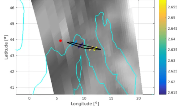
Figure 2. Illustration of a single co-location between OMI and a sunrise ZSL-DOAS measurement using the dedicated observation operator. The red dot marks the location of the ground instrument, the cyan lines indicate the coastlines of this part of the Mediter-ranean, the greyscale background contains the full orbit data and the coloured pixels are those that have their centre within the ob-servation operator (black polygon), i.e. those that are averaged to obtain a satellite measurement comparable with that of the ZSL-DOAS instrument.
3.1.2 Co-location criteria and processing
Stratospheric column
The air mass to which a ZSL-DOAS measurement is sen-sitive spans over many hundreds of kilometres towards the rising or setting Sun (e.g. Solomon et al., 1987). The co-location scheme employed here takes this into account by averaging all OMI ground pixels of a temporally co-located orbit (with a maximum allowed time difference of 12 h) that have their centre within the ZSL-DOAS observation opera-tor. This observation operator is a 2-D polygon that results from the parametrization of the actual extent of the air mass to which the ZSL-DOAS measurement is sensitive. Its hori-zontal dimensions were derived using the UVSPEC/DISORT ray tracing code (Mayer and Kylling, 2005), mapping the 90 % interpercentile range of the stratospheric vertical col-umn to a projection on the ground, and then parameterizing it as a function of the solar zenith and azimuth angles dur-ing the twilight measurement, where the SZA durdur-ing a nom-inal single measurement sequence is assumed to range from
87 to 91◦ (at the location of the station). Note that the
sta-tion locasta-tion is not part of the area of actual measurement sensitivity. The average OMI stratospheric column over this observation operator can then be compared to the column measured by the ZSL-DOAS instrument. An illustration of a single such co-location is presented in Fig. 2. Note that the above-mentioned SZA range may not be covered entirely at polar sites. For more details, we refer the reader to Lambert et al. (1996) and Verhoelst et al. (2015).
To account for effects of the photochemical diurnal
ob-tained twice daily at twilight at each station, are adjusted to the OMI overpass time using a model-based factor. The latter is extracted from LUTs that are calculated with the PSCBOX 1-D stacked-box photochemical model (Errera and Fonteyn, 2001; Hendrick et al., 2004) initiated by daily atmospheric composition and meteorological fields from the SLIMCAT chemistry transport model (Chipperfield, 1999). The ampli-tude of the adjustment depends strongly on the effective SZA assigned to the ZSL-DOAS measurements; it is taken here to
be 89.5◦. The uncertainty related to this adjustment is of the
order of 10 % or 1 to 2 1014molec. cm−2.
Tropospheric column
Regarding the tropospheric column validation, satellite data are kept if the satellite ground pixel covers the MAX-DOAS instrument location and if a MAX-DOAS measurement is within a 1 h interval centred on the satellite measurement time. The average of all MAX-DOAS measurements within this 1 h interval is taken. The typical number of MAX-DOAS measurements taken within this time interval was between two and four for most sites. This procedure was applied to
both QA4ECV OMI NO2and the OMNO2 comparisons.
3.2 Impact of quality screening
Quality screening is a necessary step before a satellite data product can be used, but it can be a limit to the data prod-uct’s scope. Figure 3a presents the remaining fractions of the satellite overpass data at the MAX-DOAS sites at each of the seven successive filter steps described in Sect. 3.1.1. Note that the Cabauw and De Bilt sites are not included, as the results are very close to that of Uccle.
With respect to the data filtering conditions mentioned ear-lier, the error flag (1) removes ∼ 10 %–30 % of the data; fil-ters on the SZA and the snow–ice flag (2 and 3) have a rel-atively small impact; the filter on the AMF ratio (4) has a large impact on the Bremen, Mainz, Cabauw, De Bilt, Uccle and Xianghe sites (35 %–40 % of data removed); and the fil-ter on CF (5) has an important screening impact at all sites (see Fig. 3), removing up to 60 % of the data at the Bujum-bura site. As an alternative to the CF filter, we also tested the CRF < 0.5 filter; for most sites the CRF and CF filters have a near-identical impact, although for Bujumbura and Nairobi the CRF filter is more restrictive (results not shown). In com-bination, the quality filters recommended by the PSD (fil-ters 1–5) remove between 56 % (Athens) and 90 % (Bremen) of the data.
Filter (6), the filter on the uncertainty component due to
cloud pressure uSAT,pc, removes 5 % of the data at most at the
Xianghe site, whereas the alternative filter on cloud pressure would have removed 15 % of the data (Fig. S1). The filter on ground pixel size (7) removes an additional 3 %–16 % of the data.
The screening can have a strong seasonal effect; for exam-ple, the winter months are strongly underrepresented for the western European urban sites (Fig. 3b). Figure 3c presents
box plots of co-located MAX-DOAS tropospheric NO2
mea-surements for each MAX-DOAS site before (black) and af-ter (blue) screening. Both the mean and median values de-crease due to the filtering step. We conclude that the quality
screening tends to reject scenes with a high tropospheric NO2
VCD, i.e. the restriction to quality-screened scenes leads to a negative sampling bias with respect to the ensemble of all scenes. On an absolute scale, the screening effect is strongest at the Xianghe site, leading to a decrease in the
yearly mean tropospheric NO2from 24 to 15 Pmolec. cm−2
(40 % decrease). At Nairobi, Thessaloniki, Bremen, De Bilt and Cabauw, the tropospheric VCD is reduced by several
peta molecules per square centimetre (Pmolec. cm−2). The
cloud filter is a main contributor to this sampling bias. This is in accordance with the results of Ma et al. (2013), who
found that higher tropospheric NO2was measured by
MAX-DOAS in Beijing under cloudy conditions compared with clear-sky conditions. Indeed, cloudy conditions lead to less
photochemical loss of tropospheric NO2, as explained by
the model results (Boersma et al., 2016). In comparisons of
OMI tropospheric NO2 with independent data, care should
be taken to ensure that the independent data are also sampled for clear-sky conditions (Boersma et al., 2016). A system-atic influence of clouds on the MAX-DOAS retrievals might contribute to the observed sampling bias effect.
It can be argued that the AMF ratio filter (filter 4) is too re-strictive. In Sect. S2 in the Supplement results are presented
for the less restrictive AMFtrop
AMFgeo ≥0.05. The remaining data
fraction is slightly increased at the Bremen, Mainz, Uccle, De Bilt and Cabauw sites (from ∼ 8 % to ∼ 10 %), and the winter months are better represented (see Fig. S2). The nega-tive sampling bias at De Bilt and Bremen is reduced, whereas it is removed at Mainz. As will be shown in Sect. 3.4.6, this adapted filtering generally has no negative impact on the satellite vs. MAX-DOAS comparisons.
3.3 Comparison of OMI stratospheric NO2with
ZSL-DOAS
Figure 4 contains time series of stratospheric NO2columns,
from both satellite (QA4ECV product) and ground-based instruments, at two illustrative ground sites: Kerguelen in the southern Indian Ocean, which is representative of very clean background conditions, and the Observatoire de Haute-Provence in France, which is affected by significant tro-pospheric pollution in local winter that often exceeds the wintertime stratospheric column. The graphs show the
well-known seasonal cycle in stratospheric NO2, which is
cap-tured similarly by satellite measurements and the ZSL-DOAS instrument. It is already evident from perusal of the results at OHP that the stratospheric comparison is hardly af-fected by the peaks in tropospheric pollution, e.g. in winter
Figure 3. Starting from satellite data with a ground pixel covering the MAX-DOAS site, panel (a) shows the remaining data fraction after the application of each of the seven filter criteria. The criteria are explained in Sect. 3.1.1. The Cabauw and De Bilt sites are not included here, as the fractions are very close to that of Uccle. Panel (b) shows the remaining fraction per month after the application of all filters. Panel (c) shows boxplots of QA4ECV MAX-DOAS data (“MXD”) co-located with QA4ECV OMI for each site, before the application of the filters (black), after the application of the filters (blue) and QA4ECV OMI co-located with MAX-DOAS after the application of the filters (“SAT”, red). The sites are sorted according to the median MAX-DOAS value before filtering. The box edges represent the 1st and 3th quartiles, the orange line represents the median, the green cross represents the mean, and the whiskers represent the 5th and 95th percentiles.
2005–2006, indicating a good separation between the tropo-sphere and stratotropo-sphere in the QA4ECV OMI retrievals.
To better reveal differences in the representation of the sea-sonal cycle, Fig. 5 presents the full time series at these two stations as a function of the day of the year (DoY), with a 1-month moving mean applied. While the seasonal cycle is generally well represented, with accurate levels in local
sum-mer, the QA4ECV OMI stratospheric NO2column does
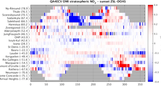
ap-pear to be a little lower than the ground-based value in local winter at these two sites. However, this is not a network-wide feature; this is illustrated in Fig. 6, which shows the median
difference for each day of the year for every station, ordered by latitude, where the median is taken over the entire 14-year time series.
From this figure, it is clear that the agreement is poorer at high latitudes, owing to more difficult measurement con-ditions (such as a high SZA) and at times a highly variable atmosphere (e.g. vortex dynamics), which amplify errors due to imperfect co-location. At more moderate latitudes, some seasonal features can be observed, but their sign varies from station to station, e.g. for Lauder and Kerguelen. A
Figure 4. (a) Time series of OMI and SAOZ stratospheric NO2above the Kerguelen NDACC station in the Indian Ocean, which is typical of clean background conditions. Panel (b) is similar to (a) but for the Observatoire de Haute-Provence (OHP), which shows more significant tropospheric columns in winter due to anthropogenic pollution.
sections at a fixed temperature. The QA4ECV NO2retrieval
includes a second-order a posteriori temperature correction to adjust for the difference in the absorption cross section between the assumed 220 K and the true effective tempera-ture (Zara et al., 2017). However, the ZSL-DOAS data were not temperature corrected, and Hendrick et al. (2012) esti-mate the impact to range between a 2.4 % overestimation in local winter and a 3.6 % underestimation in local sum-mer for ZSL-DOAS measurements at Jungfraujoch. In other words, the amplitude of the seasonal cycle should be about 6 % larger than that currently reported by the ZSL-DOAS at mid-latitudes for an assumed effective stratospheric
tem-perature of 220 K. Therefore, this effect could explain part of the discrepancy between satellite and ground-based sea-sonal cycles at sites such as Kerguelen, but it requires con-firmation with a proper ZSL-DOAS temperature correction. Developmental work on this is ongoing (François Hendrick, personal communication, 2019), but it is beyond the scope of the current paper. The excellent agreement between sunrise and sunset ZSL-DOAS measurements after mapping them to the OMI overpass time at Kerguelen suggests that the pho-tochemical adjustment works well, but it does not exclude the presence of biases that are common to sunrise and sunset measurements. At OHP, the wintertime agreement between
Figure 5. Climatological, i.e. all years mapped to a single year and with a 1-month smoothing function applied, comparison between QA4ECV OMI stratospheric NO2and the ZSL-DAOS instruments at Kerguelen and the Observatoire de Haute-Provence (OHP), revealing overall good agreement.
Figure 6. Median difference for each station (ordered by latitude) and for each day of the year, taken over the entire 14-year record, between QA4ECV OMI stratospheric NO2and the co-located, photochemically adjusted, sunset ZSL-DOAS measurements.
sunrise and sunset after photochemical adjustment is not as good. Contamination by tropospheric pollution is expected to be similar for both sunrise and sunset measurements, as it contributes to the air mass below the scattering altitude, i.e. the column above the station, as opposed to the large and offset area of sensitivity in the stratosphere. Differences be-tween sunrise and sunset contamination could still be caused by a diurnal cycle in the tropospheric column, but an analysis of that diurnal cycle (e.g. from MAX-DOAS data) is beyond the scope of this work.
Figure 7 presents the network-wide results in terms of the bias and comparison spread for each station as a function
of latitude. On average, QA4ECV OMI stratospheric NO2
seems to have a minor negative bias (−0.2 Pmolec. cm−2)
with respect to the ground-based network. In view of the
station-to-station scatter of the order of 0.3 Pmolec. cm−2
and the uncertainties on the ground-based data, this is hardly significant and is roughly in line with validation results for
other OMI stratospheric NO2data sets (e.g. Celarier et al.,
Figure 7. Meridian dependence of the mean (the circular markers) and standard deviation (±1σ error bars) of the individual differ-ences between QA4ECV (a) and STREAM (b) OMI stratospheric NO2column data and ZSL-DOAS reference data represented at in-dividual stations from the Antarctic to the Arctic. The values in the legend correspond to the mean and standard error of all mean (for each station) differences.
stratospheric NO2product, also included in the data files but
based on a very different approach (Beirle et al., 2016), does not present this negative bias (see Fig. 7b). This deserves fur-ther exploration but is outside the scope of the current pa-per. The comparison spread at a single station varies from
0.2 to 0.5 Pmolec. cm−2, corresponding to about 10 % of the
stratospheric column. Raw comparisons at Zvenigorod,
Rus-sia, yielded a higher comparison spread (1.2 Pmolec. cm−2)
due to very large pollution events in the Moscow area affect-ing the ZSL-DOAS measurements; however, for Fig. 7 these were excluded by filtering out co-located pairs with an OMI
tropospheric column larger than 3 Pmolec. cm−2.
3.4 Comparison of OMI tropospheric NO2with
MAX-DOAS
A key issue in the geophysical validation of satellite data sets with respect to suborbital reference measurements is the ad-ditional uncertainty that appears when comparing different perceptions of the inhomogeneous and variable atmosphere, i.e. when comparing data sets characterized by different sam-pling and smoothing properties, both in space and time,
which is a main topic of the European GAIA-CLIM project (Verhoelst et al., 2015; Verhoelst and Lambert, 2016). Poten-tial comparison error sources for satellite vs. MAX-DOAS are discussed in Sect. 3.4.1–3.4.5, following the framework and terminology of Verhoelst et al. (2015) and Verhoelst and Lambert (2016). The impact of the horizontal smoothing dif-ference error on the bias is presented in a qualitative way in Figs. 8 and S5–S8.
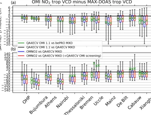
The results of the comparison of QA4ECV OMI with MAX-DOAS are provided in Sect. 3.4.6. The overall bias and dispersion are provided in boxplots of the differences for each site (Fig. 9); comparisons of the NASA OMI data prod-uct OMNO2 with MAX-DOAS are also shown. The season-ality of the bias for each site is shown in Figs. 10 and 11. Fig-ure 12 presents the overall discrepancy between QA4ECV OMI and MAX-DOAS as given by the mean-squared devia-tion (MSD), which is split into bias, seasonally cyclic and residual components. This figure also presents the consis-tency of the RMSD with the combined ex ante uncertainty. The impact of adapting screening criteria on bias and disper-sion is shown in Figs. S9–S13. A priori profile harmonization and vertical smoothing is presented in Fig. 13 for the bePRO sites at Uccle and Xianghe. The discussion of these figures is given point by point in Sect. 3.4.6. Table 3 gives an overview of the error source attributions.
3.4.1 Sources of comparison errors: overview
Part of the discrepancies between the OMI and the MAX-DOAS data sets are due to comparison errors. Starting from the general comparison equation (Verhoelst et al., 2015; Ver-hoelst and Lambert, 2016), the difference between satellite and reference measurements can be approximated in this spe-cific case as
Nv,trop,SAT−Nv,trop,REF=etotal
= −eREF+eSAT+eSr+e1r+e1t+e1z, (4)
where Nv,trop,SATand Nv,trop,REFare the tropospheric VCD
values measured by satellite and reference ground-based
sen-sors respectively, eSAT and eREF are the errors in both
mea-surements, eSr is the horizontal smoothing difference
er-ror (as the horizontal projection of the probed air mass of satellite and ground-based measurements is different), and
e1r, e1t and e1z are the horizontal, temporal and
verti-cal sampling difference error respectively (as satellite and ground-based measurement are not taken at exactly the same space and time).
3.4.2 Temporal sampling difference error
The temporal sampling difference error and the MAX-DOAS uncorrelated random error are already mitigated by averaging the MAX-DOAS measurements within a 1.0 h interval. We found that using larger time intervals can lead to an increase in the bias, which is likely due to the photochemical
evolu-tion and transport of the NO2molecule, but at this small time
window the temporal sampling difference error has a
ran-dom character3. The residual uncertainty can be estimated by
taking the uncertainty of the mean of the MAX-DOAS val-ues within each time interval. Subtracting this component in
quadrature from the RMSD, the Nv,trop,SAT–Nv,trop,REF
dis-crepancies at the different sites would be reduced by less
than 0.1 Pmolec. cm−2for the OHP, Bujumbura, Athens and
Nairobi sites, and by 0.1 to 0.5 Pmolec. cm−2at most for the
other sites. Therefore the temporal sampling difference error and the MAX-DOAS uncorrelated random error can be
con-sidered to be insignificant contributions to the Nv,trop,SAT–
Nv,trop,REFdiscrepancies, and they are not discussed further
here. In agreement with this, Wang et al. (2017) found that the impact of the temporal sampling difference error on
satel-lite vs. MAX-DOAS tropospheric NO2 VCD comparisons
was negligible.
3.4.3 Horizontal sampling difference error
Tropospheric NO2 has a large spatial variability, especially
at polluted sites; therefore, random and systematic features
in the true NO2 field at the scale of the distance between
the MAX-DOAS location and the co-located satellite ground pixel (typically a few kilometres to a few tens of kilome-tres, ∼ 10–14 km on average) can be expected. However, one must realize that (i) there is no directional preference in the co-locations, meaning that directional features are averaged out in the comparison, and (ii) the satellite measurements are strongly spatially smoothed.
To estimate the impact of the horizontal sampling
differ-ence error, we compare two sets of QA4ECV OMI NO2
tro-pospheric VCDs. Regarding the first set (Nv,trop,SAT1), it is
required that its ground pixel covers the MAX-DOAS site and its pixel centre is within 5 km of the site. The second set (Nv,trop,SAT2) has its ground pixel second-nearest to the site,
within the same overpass. SAT1pixels are within 3–4 km of
the site on average, SAT2pixels are within 11–12 km of the
site, and the distance between SAT1and SAT2pixels is
typi-cally 13.6 km, i.e. comparable to the mean distances encoun-tered in the OMI vs. MAX-DOAS comparisons. Note that
the discrepancy between Nv,trop,SAT1and Nv,trop,SAT2is due
to both the horizontal sampling difference error and the ran-dom noise error.
Details on the analysis are given in Sect. S3 in the Supple-ment. The main conclusions are as follows:
– The bias caused by the horizontal sampling difference
error reaches ∼ −0.6 Pmolec. cm−2at most (at Athens,
Bremen and Mainz) and is therefore only a very mi-nor contributor to the observed bias between OMI and MAX-DOAS (discussed later in Sect. 3.4.6).
3This is checked by comparing MAX-DOAS measurements
be-fore and after the satellite overpass time for the different overpasses.
– The dispersion of Nv,trop,SAT2−Nv,trop,SAT1can, in
prin-ciple, be due to variation in the total slant column, in the AMF or in the stratospheric slant column (see Eq. 1). It is shown in the Supplement that it is largely due to vari-ation in the slant column. It follows that uncorrelated random noise error mainly originates from the slant col-umn, not from AMF or stratospheric column (as these do not vary much between neighbouring pixels). This then justifies the use of the ex ante uncertainty
com-ponent due to SCD uncertainty, uSAT,Ns, as an estimate
of the total random error uncertainty. Note that uSAT,Ns
was scaled such that it only accounts for the random error of the slant column (Zara et al., 2018), not for sys-tematic error.
– At the Bujumbura and Nairobi sites, u2SAT
1,Ns+u
2 SAT2,Ns
exceeds the variance of the difference, indicating that uSAT,Ns is sometimes overestimated.
– The standard deviation caused by the horizontal sam-pling difference error (obtained by subtracting the dis-persion due to random noise in quadrature) is minor compared with the discrepancies encountered in the OMI vs. MAX-DOAS comparisons.
3.4.4 Vertical sampling difference error
Two sources of vertical sampling difference error can be identified. First, the surface altitude of the ground-based MAX-DOAS sensor and the mean surface altitude of the OMI ground pixel are not exactly the same. To estimate a correction, we applied a VMR-conserving vertical shift of the satellite a priori profile, described by Zhou et al. (2009). The ground levels are shifted by 0.03 km on average (Cabauw and De Bilt) to 0.4 km (Athens and Bujumbura).
This hardly changed Nv,trop,SAT−Nv,trop,REF(bias changes of
0.3 Pmolec. cm−2or less). This VMR-conserving approach
probably underestimates the discrepancy at the Athens and Bujumbura sites which have a complicated orography. The MAX-DOAS instrument at Athens is located on one of the hills surrounding the city at an altitude of 527 m, while the mean surface altitude of the co-located satellite pixels is
∼200 m. Therefore, the MAX-DOAS measurement misses
the lowest part of the tropospheric column, and correcting for this would increase the already negative bias. The MAX-DOAS instrument at Bujumbura is at an altitude of 860 m at the edge of the city, which is located in a valley surrounded by 2000–3000 m high mountains (Gielen et al., 2017); this causes the mean surface altitude of the co-located satellite pixels (∼ 1.2 km) to be higher than the MAX-DOAS instru-ment.
A second source of vertical sampling difference error is the fact that the MAX-DOAS only measures the lower
tropo-spheric NO2 VCD, whereas the satellite measures the full
tropospheric VCD. This is, in principle, a source of posi-tive bias in Nv,trop,SAT−Nv,trop,REFand, therefore, cannot
ex-plain the observed negative bias in the comparison. A proper quantification of this bias source depends critically on the as-sumed vertical profile shape and is outside the scope of the current work.
3.4.5 Horizontal smoothing difference error
Ideally, subpixel variation in the tropospheric VCD would be estimated using a high-resolution model with grid cell area comparable to the MAX-DOAS horizontally projected area of the probed air mass. Instead, we employ two semi-quantitative approaches here to estimate the bias from hori-zontal smoothing difference error.
In the first approach, the horizontal smoothing effect is
estimated from the QA4ECV OMI NO2 data. The
“super-pixel” OMI tropospheric VCDs are constructed by averaging OMI VCDs of individual pixels of a relatively small size (≤
500 km2) within a 20 km radius centred on the MAX-DOAS
site. For each overpass, a superpixel VCD is compared with the individual ground pixel VCD covering the MAX-DOAS site. Using this procedure, a superpixel consists of three in-dividual ground pixels on average. The mean difference per season, from 2004 to 2016, is presented in Fig. 8. The
sec-ond approach is similar, but uses S5P TROPOMI NO2data,
from May 2018 to May 2019, RPRO (reprocessed) + OFFL (offline) data with processor version 01.02.00–01.02.02, and the superpixel tropospheric VCD is constructed by averag-ing VCDs of individual pixels that are within a latitude,
lon-gitude box of 1lat = 0.14◦, 1long = 0.7◦ centred on the
MAX-DOAS site for each overpass. TROPOMI has a sim-ilar overpass time to OMI (early afternoon) and a
consider-ably finer resolution (3.5 × 7 km2at nadir). The area of this
superpixel corresponds to ∼ 700–900 km2, i.e. about the size
of a bigger OMI pixel, and typically contains 20 TROPOMI ground pixels.
The OMI-based approach has as the advantage that the time range is appropriate, but it is limited by the large ground pixel size. Regarding the finer resolution TROPOMI data, one should keep in mind that its ground pixel size is still large compared with the horizontally projected area of the
probed air mass of the MAX-DOAS4; hence, the
contribu-tion of the horizontal smoothing difference error to the bias and comparison might still be underestimated. Another lim-itation is that the TROPOMI time range considered does not overlap with the time range considered for OMI. Both ap-proaches suggest a negative bias contribution due to the hor-izontal smoothing difference error at the Mainz and Thessa-loniki sites and no such bias contribution at OHP, whereas
4The horizontal distance of the QA4ECV MAX-DOAS
mea-surements is small compared with a TROPOMI pixel in both the viewing and the perpendicular direction. Regarding bePRO MAX-DOAS, although it has a small field of view, its probed distance in the viewing direction (∼ 10 km) is of similar or slightly larger magnitude compared with the cross section of a TROPOMI ground pixel.
the results are mixed for other sites (the bias varies over the seasons, and/or different results are found between the OMI-and TROPOMI-based calculations). Differences between the OMI- and TROPOMI-based calculations are likely caused by (i) the much larger central pixel of OMI compared with TROPOMI, which leads to a lower sensitivity to fine-scale variations in Fig. 8a, and (ii) the evolution in parameters
such as NO2concentration patterns, which are captured
dif-ferently by the different temporal ranges used in Fig. 8a and b. A case in point is the positive mean differences in JFM (January–February–March) and OND (October–November– December) captured in the TROPOMI-based calculation but not in the OMI-based calculation. Both MAX-DOAS sensors are not located in urban centres, although pollution centres are located nearby. Therefore, the positive mean differences in JFM and OND captured by TROPOMI are likely due to
NO2 fields in the periphery of the TROPOMI superpixel.
This is in agreement with the very recent work by Pinardi et al. (2020) on the horizontal smoothing effect. The esti-mated “horizontal dilution factors” in Fig. S3 of Pinardi et al. (2020) are positive for Cabauw and Xianghe, indicating that
NO2is higher on the periphery than at the MAX-DOAS
lo-cation.
A tropospheric NO2monthly field with subpixel
variabil-ity is derived from the QA4ECV OMI NO2 data using a
variant of the temporal averaging approach of Wenig et al.
(2008)5(as shown in Figs. S5–S8) for months with a minimal
(left column) and maximal (right column) OMI vs. MAX-DOAS bias (as derived from Figs. 10–11). Fields are con-structed for each month by averaging over the 2004–2016 period. The resulting field is horizontally smoothed; the
vari-ability is an underestimate of the true horizontal NO2
vari-ability. Subpixel enhanced tropospheric NO2approximately
centred on the MAX-DOAS site can be identified in high-bias months at Nairobi, Thessaloniki and Mainz, whereas this is clearly not the case for the OHP, Bujumbura, Uccle, De Bilt/Cabauw and Xianghe sites. In Athens the pollution peak centre is some 10 km from the sensor, and for Bremen no clear peak is identified.
The contribution of the horizontal smoothing difference error to the (OMI–MAX-DOAS) bias at Mainz is consistent with the results of Drosoglou et al. (2017), who achieved a significant bias reduction by adjusting the OMI data with fac-tors derived from air quality simulations at a high spatial res-olution of 2 km.
Similar maps have been constructed in studies such as Ma et al. (2013) and Chen et al. (2009) to estimate the impact of the horizontal smoothing effect on satellite vs. DOAS com-parisons.
5Here, the arithmetic average of covering satellite ground pixels
is taken for each 0.02 × 0.02 grid cell rather than using a weighted average, as done by Wenig et al. (2008). Only ground pixels with an area less than 950 km2are considered.
Figure 8. (a) Mean difference for each season between the QA4ECV OMI superpixel (ground pixels averaged within 20 km of the central site) and the central OMI ground pixel using data from 2004 to 2016. (b) Similar to (a) but using TROPOMI NO2data from April 2018 to
May 2019, and the superpixel is defined within a latitude, longitude box of 1lat = 0.14◦, 1long = 0.7◦centred on the MAX-DOAS site.
3.4.6 Comparison results
Bias and dispersion
Figure 9 (black boxplots) presents boxplots of the differ-ence of QA4ECV OMI with co-located QA4ECV MAX-DOAS for each MAX-MAX-DOAS site. At all sites, the bias of QA4ECV OMI with respect to QA4ECV MAX-DOAS is negative. On an absolute scale, it is the lowest at the less polluted OHP and Bujumbura sites (mean difference
of −0.9 and −1.7 Pmolec. cm−2 respectively), and highest
at the Thessaloniki and Mainz sites (mean difference of
∼ −4 Pmolec. cm−2). On a relative scale, the bias is
low-est (median relative difference between −15 % and −20 %) at the Uccle, Cabauw, De Bilt and Xianghe sites and high-est (median relative difference of ∼ −70 %) at Bujumbura and Nairobi. The difference dispersion, expressed as the in-terquartile range (IQR), is lowest at the Bujumbura, OHP and
Nairobi sites (∼ 1–2 Pmolec. cm−2) and largest at the Mainz
and Xianghe sites (∼ 5–6 Pmolec. cm−2).
As discussed in Sect. 3.4.2–3.4.5, among the different comparison error components, only the horizontal smoothing difference error is expected to induce an important negative bias, and this is only true for some sites (e.g. Thessaloniki and Mainz), whereas for other sites (e.g. OHP and Xianghe) this is not expected. This means that the bias is (at least in some cases) due to error in the satellite and/or MAX-DOAS measurement, not due to comparison error.
We present in the same figure boxplots of the tropospheric
NO2VCD difference between OMNO2 data and QA4ECV
MAX-DOAS measurements (blue boxplots). The bias of OMNO2 vs. QA4ECV MAX-DOAS is comparable to that
of QA4ECV OMI NO2vs. QA4ECV MAX-DOAS, although
slightly more negative at all sites except Cabauw. If one only
considers the subset of the OMNO2 pixels where QA4ECV OMI has an accepted pixel, the OMNO2 bias becomes closer to that of QA4ECV OMI for most sites. Although bePRO MAX-DOAS has a better correction for aerosols and vertical profile effects compared to QA4ECV MAX-DOAS in princi-ple, the bias of QA4ECV OMI with respect to bePRO MAX-DOAS (Fig. 9, green boxes, only for the Bujumbura, Uccle and Xianghe sites) is comparable to that of QA4ECV OMI vs. QA4ECV MAX-DOAS.
In most cases, we conclude that mutual differences
be-tween the tropospheric NO2 VCD of the two OMI
satel-lite data products and between both MAX-DOAS processing methods are small compared with the differences between the satellite OMI data products and the MAX-DOAS mea-surements. The main exception is at OHP, where the median difference and relative difference of OMNO2 vs. QA4ECV
MAX-DOAS (−1.4 Pmolec. cm−2, −60 %) is considerably
more negative than that of QA4ECV OMI vs. QA4ECV
MAX-DOAS (−0.8 Pmolec. cm−2, −30 %). The observation
of higher MAX-DOAS tropospheric VCD compared with satellite measurements is a common finding in the literature (e.g. Ma et al., 2013; Kanaya et al., 2014; Chan et al., 2015; Jin et al., 2016; Drosoglou et al., 2017, 2018). Therefore, the negative bias is not specific to a particular satellite or MAX-DOAS data product.
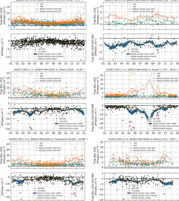
Seasonal cycle of the bias
Figures 10 and 11 present a seasonal plot (i.e. all data
mapped to 1 year) of QA4ECV OMI tropospheric NO2VCD,
of QA4ECV MAX-DOAS, and of the difference for each site. Also indicated are the rolling monthly mean and median as well as outliers identified by iterative 4σ clipping.