Pollinator species richness: Are the declines slowing down?

HAL Id: hal-01408957

https://hal.sorbonne-universite.fr/hal-01408957

Submitted on 5 Dec 2016

HAL is a multi-disciplinary open access archive for the deposit and dissemination of sci-entific research documents, whether they are pub-lished or not. The documents may come from teaching and research institutions in France or abroad, or from public or private research centers.

L’archive ouverte pluridisciplinaire HAL, est destinée au dépôt et à la diffusion de documents scientifiques de niveau recherche, publiés ou non, émanant des établissements d’enseignement et de recherche français ou étrangers, des laboratoires publics ou privés.

Distributed under a Creative Commons Attribution| 4.0 International License

down?

Tom Van Dooren

To cite this version:

Tom Van Dooren. Pollinator species richness: Are the declines slowing down?. Nature Conservation-Bulgaria, 2016, pp.11-22. �10.3897/natureconservation.15.9616�. �hal-01408957�

Pollinator species richness:

Are the declines slowing down?

Tom J. M. Van Dooren1,2

1 Naturalis Biodiversity Center, Darwinweg 2, 2333 CR Leiden, The Netherlands 2 CNRS - UMR 7618

Institute of Ecology and Environmental Sciences (iEES) Paris, Université Pierre et Marie Curie, Case 237, 7 Quai St Bernard, 75005 Paris, France

Corresponding author: Tom J. M. Van Dooren (tvdooren@gmail.com)

Academic editor: K. Henle  |  Received 20 June 2016  |  Accepted 11 July 2016  |  Published 22 September 2016

http://zoobank.org/ECD71ECF-842D-4E87-AB97-50C8C03B4F48

Citation: Van Dooren TJM (2016) Pollinator species richness: Are the declines slowing down?. Nature Conservation 15:

11–22. doi: 10.3897/natureconservation.15.9616

Abstract

Changes in pollinator abundances and diversity are of major concern. A recent study inferred that pollina-tor species richnesses are decreasing more slowly in recent decades in several taxa and European countries. A more careful interpretation of these results reveals that this conclusion cannot be drawn and that we can only infer that declines decelerate for bees (Anthophila) in the Netherlands.

Keywords

Species richness, rarefaction, pollinators, species accumulation curve, diversity decline

Introduction

In a recent paper investigating different plant and pollinator groups in three countries, Carvalheiro et al. (2013, CA2013 hereafter) conclude that “Over more recent decades [...] declines in species richness [...] slowed down for many of the studied taxa and countries”, a statement subsequently expressed less firmly as “past declines in some pol-linator groups may have recently slowed or even partially reversed” (Kunin 2013). This conclusion on decelerating declines has been adopted in the recent UN IPBES Pol-lination Report draft summary (Potts et al. 2016, status “established but incomplete”). Carvalheiro and co-authors (2013) rightly state that a general deceleration would be

Copyright Tom J. M. Van Dooren. This is an open access article distributed under the terms of the Creative Commons Attribution License (CC BY 4.0), which permits unrestricted use, distribution, and reproduction in any medium, provided the original author and source are credited.

highly relevant for conservation biology and biodiversity management and suggest in their concluding remarks that European Union (EU) policy could have played a role in the effect they infer. Ambitions in terms of biodiversity management seem reduced in recent EU legislation (Pe’er et al. 2014), unproblematic if the loss of diversity al-ready slows down. I reassess the CA2013 statement that species richness declines have decreased in magnitude for many taxa and countries. The data and statistics presented in that publication are considered, as well as elements of the scripts provided by the authors to anyone interested. My own scripts used to carry out this assessment using R (R Core Team 2015) are available upon request.

Inference of decelerating declines in CA2013

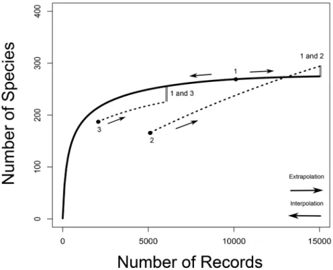
The analysis in CA2013 is based on comparisons of species accumulation curves (Col-well et al. 2012) between periods (Figure 1). These curves express the dependence of the number of species in a sample on a variable representing sampling effort, and the horizontal asymptote of the curve is species richness. The comparisons in CA2013 are between three 20-year periods (1950–1969, 1970–1989 and 1990–2009). Per pair of successive periods, richness change was estimated as the difference between the log transformed numbers of species in the second minus the first period, where these numbers of species were predicted at a sampling effort (number of records) specific to each difference. Differences were calculated per group of species, country or per grid cell at smaller spatial scales. The differences between logged numbers of species were predicted at three times the numbers of records of the least sampled period, either by extrapolation when numbers of records in both periods were smaller than that, or by inter- and extrapolation combined (Fig. 1). The standard deviation of each difference was estimated using a bootstrap approximation. For spatial scales with multiple grid cells, random effects models that use squared standard deviations as the known error variances (Viechtbauer 2010) were fitted to the estimated changes per grid cell. The average effect across grid cells was used as a measure of richness change. As a check of robustness of results, the analysis was repeated with only interpolation (rarefaction) or only extrapolation and also with standard deviations of the logged difference estimated with an analytical expression (Colwell et al. 2012, CA2013). CA2013 inferred that rates of decline have decreased from observing that estimates became less accentuated, or that significant species number increases occur between the most recent periods when there had been a decrease before. Per taxon and country, Table 1 lists the state-ments from the text that the authors used to support their conclusion of a decelerating decline in species richness in several taxa and countries. All statements in the table can be found in CA2013’s Results section on changes since 1990. When a spatial scale is mentioned in CA2013, I list the spatial scales to which the statement applies. Eight out of fifteen taxon/country combinations have statements in support of a decelerating decline. CA2013 state that this is independent of the way in which they carried out the analysis, hence robust.

Figure 1. Species accumulation curves. Species richness is the asymptote of a species accumulation curve, which expresses the dependence on sampling effort of the number of species sampled from an assemblage. In CA2013, sampling effort is given by the number of records from which the number of species is calculated. For illustrative purposes, an example with three arbitrary samples (for 10000, 5000 and 2000 records, labeled from one to three) is drawn. For sample one, a predicted species accumulation curve is added that gradually increases from one species sampled to the predicted species richness for that assemblage (full line). Such curves are constructed on the basis of interpolation and extrapolation. For samples two and three only segments of extrapolated curves are drawn (dotted lines). For sample two, a curve that crosses the species accumulation curve of sample one is sketched. For samples one and three species accumulation curves are more or less proportional. The way in which the species richness differ-ences between samples are assessed in CA2013 is illustrated by indicating on the species accumulation curves at which numbers of records pairwise comparisons would be made between two sample pairs (1 vs. 2 and 1 vs. 3). The number of species of the sample with the smallest number of records is extrapolated to the number expected at three times the number of records. When the number of records of the other sample is still larger than that, the number of species of the second sample is interpolated (rarefied), oth-erwise it is extrapolated as well.

A reassessment is required

Note that species richness was nowhere estimated in CA2013, rather numbers of spe-cies at particular finite sampling efforts were used as proxies for spespe-cies richness.

As Table 1 shows, CA2013 does not contain any test for differences in rates of richness change between the pairs of twenty-year time periods considered. They did

not aim to reject the null hypothesis that species numbers change at a constant rate. One cannot infer a change in species number decrease by checking which confidence intervals overlap with zero change and which ones not. For example if confidence intervals for declines would have been [-2, -0.2] between the first pair of twenty-year periods and [-1, 0.2] between the second pair, these intervals should not be interpreted as evidence of a change in decline as they do overlap, while the estimates would indeed have become less accentuated.

While appropriate tests for a slowing down of richness decline are lacking in CA2013, we can still check ourselves whether confidence intervals for changes overlap between interval pairs, and conclude on the significance of decelerations in species richness from the absence of overlaps.

Table 1. Statements in CA2013 supporting a slowing down of species richness decline. The column with spatial scales to which a statement applies lists either the grid sizes (as length of a grid side in km) or the country level. $: The changes on Figure 1 and in Table S2 are in fact decreases. *: It is unclear if this result is interpreted as a slowing down of the decline, since no significant change between the first two periods is reported. For all other groups with statements, a decline in an earlier period is reported.

Species group/Country Statement on the change between _{the two most recent periods} Spatial scale Non-Bombus bees

Belgium – –

Great Britain Significant increase 10/20/40/80/160 Netherlands Significant increase 10/20/40/80 Bumblebees

Belgium – –

Great Britain Declines less accentuated – Great Britain Significant increase Country level Netherlands Declines less accentuated

Butterflies

Belgium – –

Great Britain – –

Netherlands Declines less accentuated 10/20 Netherlands Significant increase$ _10/20

Hoverflies

Belgium Significant increase* _–

Great Britain – –

Netherlands – –

Plants

Belgium – –

Great Britain Recovery of species richness 10/20/40 Netherlands Recovery of species richness Country level

Methods

I assess limits of confidence intervals in tables and figures of CA2013 to construct tests for a significant deceleration in richness decline. When these numbers are provided, limits of intervals are calculated from parameter estimates and their standard devia-tions using the normal approximation for 95% intervals (z = 1.96), otherwise limits of confidence intervals in the figures are inspected. I will conclude that a species rich-ness decline has slowed down when (1) there is a significant species richrich-ness decrease between the first two periods. In terms of the analysis of CA2013 that translates into a negative response variable for the change between the first two periods, with a con-fidence interval that does not overlap zero. (2) The species richness decrease becomes less. The confidence interval in CA2013 for the change between the last two periods does not overlap with that for the previous two periods, and the estimate is larger.

I believe that the parallel analyses in CA2013 with different estimators of species number variance, for rarefaction and for extrapolation are to some extent a valid way of assessing the robustness of the inference. Comparing results when differences are predicted at different numbers of records implicitly checks whether crossing species accumulation curves might be present. With such crossings, the sign of species num-ber differences will depend on the numnum-ber of records where the difference is assessed (Fig. 1, comparison sample 1 vs. 2). I will require that decelerating declines, which are detected when combinations of inter- and extrapolation are used, also need to be detected for extrapolation to be considered robust.

Unfortunately, the robustness assessment in CA2013 is affected by anti-conserv-ative inference, duplications of statistics and errors as explained in the following sec-tions, such that a number of assessments are removed from consideration. This makes the assessment of robustness more limited than originally intended.

In the reassessment, I will give less importance to results at smaller spatial scales than at country level. First of all, the conclusion re-investigated here was formulated at country level. Second, for comparisons at smaller scales sample sizes are smaller. Hence the risk that predicted species numbers badly reflect species richness can be in-creased. Third, there is no guarantee and no evidence that the local grid cells compared between the first two and the last two periods are the same or samples from sets with identical properties. Fourth, I will show below that regression corrections carried out in CA2013 for the smaller spatial scales carry an additional risk of anticonservative inference and bias.

Increased risk of anti-conservative inference

In part of their calculations, CA2013 have used a bootstrap estimate of the variance of predicted species number. After inspection of the R code used, it turns out that their estimate is neither bootstrap variance nor bootstrap accuracy (e.g., Walther and

Moore 2005), so not a regular bootstrap estimate of variance. In their paper as pub-lished before correction, they sum the absolute value of the bootstrap estimated bias and the squared bootstrap average of Colwell et al.’s (2012) expression for the standard deviation of predicted species richness. CA2013 intended the bootstrap to account for additional uncertainty caused by potential non-random sampling, thus variances “corrected” in this manner should rarely become smaller than the analytical expression based on multinomial sampling. However, simulations using samples from the EIS bee and bumblebee dataset used in CA2013 indicate that they often do.

CA2013’s script contained a calculation error: the bias on species number in the earlier period is used in calculations where it should have been that of the later period. In a modified script distributed with their corrigendum (Carvalheiro et al. 2013b) and used to produce a modified Figure 1, this error has been corrected. At the same time, however, a second change has been implemented: the bootstrap standard deviation of species number is now calculated as the product of the bootstrap average of the estimate of standard deviation based on multinomial sampling, times a scaling factor which is equal to one plus the absolute value of the ratio of the bootstrap estimated bias in predicted species number divided by the original estimate of species number. In my simulations, this quantity is smaller than the analytical expression in over 90% of samples simulated using random (multinomial) draws from the EIS bee data species distribution. As the CA2013 bootstrap confidence intervals are obtained using non-standard approaches, we know little about their performance in frequentist inference, except for the simulations I mention here which suggest that they have undesirable properties that lead to anticonservative inference.

The unweighted tests in Table S5 of CA2013, where we expect standard deviations to be calculated automatically from the data variances, all use averages of the bootstrap standard deviations as weights. They are therefore all weighted in an unexpected man-ner and should not be considered.

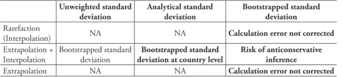
In Table S5 of CA2013, the three listed tests per taxon/country for effects at the national scale are in fact always the same test pasted in three times, namely the test based on a bootstrapped variance estimate. The R script of the authors does not con-tain any calculations for non-bootstrap weighted tests for national data, such that there is no robustness assessment possible. An unweighted test is impossible to carry out at the national level, as there are too few values to calculate data variances per species group/country. I am forced to rely solely on CA2013’s bootstrap statistics for the country-level comparisons. Statistics in Tables S2 and S5 of CA2013 and the sup-plementary figures have not been adapted to the new heuristic to estimate bootstrap standard deviation, we therefore need to inspect the corrected Figure 1 of CA2013 to assess comparisons based on bootstrapped statistics and the uncorrected figures of the supplement (by comparing plotted limits of confidence intervals with a ruler). Table 2 summarizes the different estimates CA2013 provides and problems arising when one wants to use them further. A proper assessment of robustness is difficult, as in fact nearly any category of estimates either has uncorrected errors, is not provided, or not available at the national level. Nevertheless, I will use rarefaction and extrapolation

Table 2. Species number statistics. CA2013 presents standard deviations of species number change es-timated in different ways and at different sampling efforts (NA: not available). Each of these statistics available from the paper or its figures is calculated in an unexpected manner. Categories where remarks are in bold are used for the reassessment.

Unweighted standard deviation Analytical standard deviation Bootstrapped standard deviation Rarefaction

(Interpolation) NA NA Calculation error not corrected Extrapolation +

Interpolation Bootstrapped standard deviation deviation at country levelBootstrapped standard Risk of anticonservative inference Extrapolation NA NA Calculation error not corrected results in my assessment, and will proceed as if their standard deviations had been correctly calculated. When such estimates will affect conclusions, I will note whether the uncorrected standard deviations play an important role in that or whether just the estimates of species number change would lead to the same conclusion.

Bias

CA2013 assume that their response variable (log-ratio of predicted species numbers at a particular sampling effort) is directly comparable between different sampling ef-forts. This is only expected when non-linear species accumulation curves for different periods are proportional and will often not hold good when these curves for example cross (Fig. 1).

CA2013 call it a bias that their response variable often becomes larger with larger differences in data sample sizes between periods. To correct for this presumed bias, they included the difference of the logged numbers of records in the two time periods as covariate in the random effects models. That the difference in species number often becomes larger with larger differences in sample sizes is an absolutely normal pattern if species accumulation curves are not proportional and sample sizes where species num-bers are interpolated are not randomly distributed (for example consistently smaller in one period). It is not difficult to sketch a pair of species accumulation curves where unbiased estimation and a non-random set of sample sizes per period would produce this pattern. Applying the proposed regression correction here would distort the pat-tern of real differences. On the other hand, we also need to check whether it removes estimation bias when differences are calculated between different samples from the same assemblage.

Simulating data from a single species accumulation curve based on the EIS bee data, I found that the “regression correction” approach CA2013 used in their analysis of species richness change patterns at spatial resolutions smaller than the national scale does not remove bias on the intercept. When the ratio of sample sizes between periods is on average different from one in these simulations, tests on the intercept or on the

partial residuals used in this regression approach too often conclude that species ac-cumulation curves have changed. These tests have anticonservative amounts of type I errors and also show estimation bias. When the sample in the second period is on average larger (smaller), the intercept is negative (resp. positive).

Additionally, the variances of partial residuals used for “corrected” per-grid tests in CA2013 were not taking variances of estimated regression parameters into account neither the random effect variance of the model fitted (Viechtbauer 2010). Also here, simulations indicate that the variance used is often smaller than that of the partial residual when calculated correctly. Thus tests on small spatial scale differences can be expected to be anticonservative due to a biased estimator and underestimated errors, even if the regression correction were appropriate. This completes my arguments to give sub-national analyses much less importance. I will focus on the tests at the nation-al level as much as possible, even while anticonservative inference is expected there too.

Further irregularities

There are further irregularities in the analysis of CA2013. In the functions used to predict species accumulation curves, which I originally wrote, zero values have been replaced by positive numbers, and where functions should produce missing values or zeroes, shortcuts have been inserted that return other values. The threshold for the rma. uni() function used for weighted regression is not set at the default value of 10^-5 but at 0.01, which makes convergence of the algorithm on a decent estimate of unexplained heterogeneity in the data uncertain. In one instance, a 0.06 tail probability is used to conclude on significance of a test and not 0.05 as would be standard. Numbers of cells significantly declining or increasing in Tables S2 and S5 of CA2013: The authors have applied a two-sided test, not one-sided ones. They have counted as significant declines cells that had tail probabilities below 0.05 for that two-sided test and with a negative log-ratio value. These are thus not one-sided tests at 5% level as suggested by the verbal statement, but one-sided tests at the 2.5% significance level. The numbers of signifi-cant increasing cells are wrong altogether. Authors have counted number of grid cells with tail probabilities above 0.05 and a positive coefficient as significant, instead of the cells with a probability below 0.05. This error is made for all weighting methods, inter- and extrapolation. Thus entire columns “significant increases” are wrong.

Results

From the comparisons of confidence intervals extracted from CA2013’s corrected Fig-ure 1 and from the supplementary tables and figFig-ures, I conclude the following. For only six country/taxon combinations, confidence intervals of earlier rates of change are below zero and these of earlier and recent rates of change do not overlap in at least one test at the national level (Table 3). There are thus at most six combinations that need

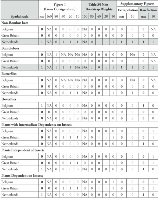
Table 3. A reassessment of results in CA2013. Confidence intervals are extracted and calculated from figures and tables in CA2013. Cells with value “1” indicate taxa and countries where a significant decline in number of species between the two first periods is followed by a change in species number between the two most recent periods, which is significantly less negative (with non-overlapping 95% confidence intervals). Columns “nat” indicate comparisons at the national level and are in bold. I attach a larger im-portance to them as explained in the text. “NA” indicates missing values, where some data were lacking to carry out the comparison. Rows for which I would conclude from CA2013 that there is a decreased decline (provided that further inference problems are ignored) are in grey.

Spatial scale

Figure 1

(From Corrigendum) Bootstrap WeightsTable S5

Non-Supplementary Figures Extrapolation Rarefaction

nat 160 80 40 20 10 160 80 40 20 10 nat 10 nat 10

Non-Bombus bees Belgium 0 NA 0 0 0 0 NA 0 0 0 0 0 0 0 NA Great Britain 0 0 0 0 0 0 0 0 0 0 0 0 0 0 0 Netherlands 1 NA 0 1 1 1 NA 0 1 1 1 1 1 1 1 Bumblebees Belgium 0 NA 1 NA NA NA NA 0 0 0 0 0 NA 0 NA Great Britain 0 0 1 0 0 0 0 0 0 0 0 0 0 0 NA Netherlands 1 NA 1 1 1 NA NA 1 0 1 1 1 1 0 1 Butterflies Belgium 0 NA 0 NA NA NA NA 0 0 0 0 0 NA 0 NA Great Britain 0 0 0 0 0 0 0 0 0 0 0 0 0 0 0 Netherlands 0 NA 0 0 1 1 NA 0 0 1 1 0 1 0 0 Hoverflies Belgium 1 NA 0 0 0 0 NA 0 0 0 0 0 0 1 0 Great Britain 0 0 0 0 0 0 0 0 0 0 0 0 0 0 0 Netherlands 0 NA 0 0 0 0 NA 0 0 0 0 0 0 0 0

Plants with Intermediate Dependence on Insects

Belgium 0 NA 0 0 0 0 NA 0 0 0 0 0 0 0 1

Great Britain 0 0 0 1 1 1 0 0 1 1 1 0 0 0 1

Netherlands 0 NA 0 0 0 0 NA 0 0 0 0 0 0 1 0

Plants Independent of Insects

Belgium 0 NA 0 0 0 0 NA 0 0 0 0 0 0 0 1

Great Britain 0 0 0 0 1 1 0 0 0 1 1 0 0 0 1

Netherlands 1 NA 0 0 0 0 NA 0 0 0 0 0 0 1 0

Plants Dependent on Insects

Belgium 0 NA 0 0 0 0 NA 0 0 0 1 0 0 0 1

Great Britain 0 0 0 1 1 1 0 0 1 1 1 0 0 0 1

further scrutiny, to check whether the decelerating decline suggested in at least one test might be there with some robustness.

For bumblebees and other bees in the Netherlands, the pattern is found in Figure 1 of CA2013, for extrapolation, at smaller spatial scales and for rarefaction

(non-Bombus bees). This seems the most robust evidence for a decrease in biodiversity loss

in CA2013, given the choice of inference method, and assuming anti-conservative approaches and calculation errors have limited effect. For three groups of plants in the Netherlands, the tests are significant when rarefying species numbers. The signifi-cance disappears in one group in Figure 1 of CA2013 and completely for extrapo-lation and at smaller spatial scales. For extrapoextrapo-lation, the estimates are not species number decreases. I conclude that this evidence on a reduced loss is non-robust and could be due to crossing species accumulation curves. For hoverflies in Belgium, the difference is significant at the national level for the new Figure 1, but not signifi-cant for spatial levels below national and not for the extrapolation. The estimates of species number change are all positive for extrapolation. I conclude that this result is not robust and could be due to crossing species accumulation curves. Plants in Great Britain at the smallest spatial scales suggest a reduced rate of changes, but the results for larger spatial scales are not significant. The same holds for butterflies in the Netherlands.

Taken together, the inference in CA2013 only provides robust inference of a slow-ing down of species richness decline in two out of fifteen taxon/country combinations. This is in fact one taxon, the bees Anthophila, in a single country, the Netherlands.

Discussion

Table 1 illustrates that CA2013 does not contain a test for a slowing down of species richness decline. When I construct such tests based on the confidence intervals pro-vided in the paper (Table 2), and apply the procedure to check robustness proposed by the authors as much as possible, only two out of fifteen taxon/country combinations show evidence of decelerating declines. If I would have given the analyses at small spa-tial scales the same weight in my assessment as the country level, the conclusion would be slightly different. Butterflies in the Netherlands at the smallest spatial scale show a decelerating decline, which is also detected when an analytical expression for species number variance is used, and for extrapolation. If we conclude that this is evidence of a decelerating decline, we would then have detected it for two taxa in a single country. However, on top of arguments given in the previous sections, the data on butterflies in the Netherlands show a massive increase in numbers of records between periods (from 29,496 records to 162,102 and 1,835,545; CA2013 Table S1) and for the second esti-mate of richness change, 40% more 10 km grid cells are used than for the comparison of the first two periods. Figure S1.1 of CA2013 suggests that these 40% are not ran-domly distributed. I therefore conclude that this comparison at small spatial scales is insufficiently reliable to be presented as evidence.

Alternatively, we could forgo trying to draw conclusions on the separate species groups and countries altogether and just inspect estimates and the relative occurrence among them of species number decreases between the first two periods, and whether the last periods would often have increased values for species number change relative to the previous period. Such an approach would be akin to CA2013’s statements that estimates have become less accentuated. Please note that such a procedure would be sensitive to estimation bias. At the same time, we would assume that all data hetero-geneity can be ignored. Note that this inspection can easily generate bias itself: We should not select a subset of data points with negative changes between the first peri-ods to assess further. In the case of independent changes between pairs of periperi-ods, just inspecting groups with the smallest values between the first pair of periods would bias the estimates for the second pair of periods to be larger than the first more often. Nei-ther should we use all estimates provided in CA2013, as estimates for different spatial scales on the same group are not independent but re-calculations on the same data. If we count the changes at the national level from the corrected Figure 1 and the sup-plements, we do find decreases relatively often (15/21 estimates negative), and many more positive (less negative) recent changes (15/21 changes larger than between first periods). However, this pattern is again not robust. For extrapolated estimates, the de-creases are a minority (8/21 estimates negative) and the estimates of recent change are not more often positive than what one could expect by chance (12/21 estimates larger). Sign tests (Conover 1999) could be used to test null hypotheses on these counts, but the raw numbers already show that we would have only weak support for a conclu-sion that the median species number decline become smaller. The lack of robustness points again to the possibility that results found in the data can be due to changes in the shapes of species accumulation curves. This approach and the hypotheses it can test would not allow us to draw conclusions on declines in individual countries and taxa. This is possible when considering standard deviations of the estimates as was done above. These standard deviations also allow us to distinguish more reliable estimates from less reliable ones, when calculated correctly and appropriately.

My reassessment and the brief discussion of what a simplified analysis and hypoth-esis testing scheme would provide do accept the inference method based on extrapolat-ing and rarefyextrapolat-ing species numbers as valid. One can argue against that. Species richness-es were not richness-estimated in CA2013, and the paper did not provide statistics that allowed tests at the country level without using bootstrap estimates of standard deviations. The time period was arbitrarily binned in three time intervals. If declines and decelerations occur, they don’t have to be synchronous across taxa and countries and match with the time intervals. Moreover, O’Hara (2005) has stated that “Estimating species richness [...] seems futile, as it is impossible to know how bad the estimates are”, pointing out known general difficulties with assessing bias and precision of species richness esti-mates. Given these additional arguments regarding the type of analysis CA2013 used, a new analysis using different methods still seems warranted and could further adjust the present conclusion. Therefore the status of the statement on decelerating declines in the Pollination Report (Potts et al. 2016) should be adjusted accordingly.

Acknowledgements

I thank Menno Reemer for providing the EIS (Invertebrate Survey Netherlands) bee data-set. An anonymous peer provided extremely useful comments through Peerage of Science.

References

Biesmeijer JC et al. (2006) Parallel declines in pollinators and insect-pollinated plants in Britain and the Netherlands. Science 313: 351–354. doi: 10.1126/science.1127863

Carvalheiro LG et al. (2013) Species richness declines and biotic homogenisation have slowed down for NW‐European pollinators and plants. Ecology Letters 16: 870–878. doi: 10.1111/ele.12121

Carvalheiro LG, Kunin WE, Biesmeijer JC (2013b) Corrigendum to Carvalheiro et al. (2013). Ecology Letters 16: 1416–1417. doi: 10.1111/ele.12175

Colwell RK, Chao A, Gotelli NJ, Lin S-Y, Mao CH, Chazdon RL, Longino JT (2012) Models and estimators linking individual-based and sample-based rarefaction, extrapolation, and comparison of assemblages. Journal of Plant Ecology 5: 3–21. doi: 10.1093/jpe/rtr044 Conover WJ (1999) Practical Nonparametric Statistics (3rd _{eds). Wiley, 592 pp. http://eu.wiley.}

com/WileyCDA/WileyTitle/productCd-0471160687.html

Kunin WE (2013) No bias behind pollinator research. Nature 502: 303. doi: 10.1038/502303a O’Hara RB (2005) Species richness estimators: how many species can dance on the head of a

pin? Journal of Animal Ecology 74: 375–386. doi: 10.1111/j.1365-2656.2005.00940.x Pe'er G, Dicks LV, Visconti P, Arlettaz R, Báldi A, Benton TG, Collins S, Dieterich M, Gregory

RD, Hartig F, Henle K (2014) EU agricultural reform fails on biodiversity. Science 344: 1090–1092. doi: 10.1126/science.1253425

Potts SG, Imperatriz-Fonseca V, Ngo HT, Biesmeijer JC, Breeze TD, Dicks LV, Garibaldi LA, Hill R, Settele J, Vanbergen AJ (2016) IPBES: Summary for policymakers of the assess-ment report of the Intergovernassess-mental Science-Policy Platform on Biodiversity and Ecosys-tem Services on pollinators, pollination and food production. http://www.ipbes.net/sites/ default/files/downloads/Pollination_Summary%20for%20policymakers_EN_.pdf R Core Team (2015) R: A language and environment for statistical computing. R Foundation

for Statistical Computing, Vienna, Austria. https://www.R-project.org/

Viechtbauer W (2010) Conducting meta-analyses in R with the metafor package. Journal of Statistical Software 36: 1–48. doi: 10.18637/jss.v036.i03

Walther BA, Moore JL (2005) The concepts of bias, precision and accuracy, and their use in testing the performance of species richness estimators, with a literature review of estimator performance. Ecography 28: 815–829. doi: 10.1111/j.2005.0906-7590.04112.x