HAL Id: hal-02907062
https://hal.laas.fr/hal-02907062
Submitted on 27 Jul 2020
HAL is a multi-disciplinary open access
archive for the deposit and dissemination of sci-entific research documents, whether they are pub-lished or not. The documents may come from teaching and research institutions in France or abroad, or from public or private research centers.
L’archive ouverte pluridisciplinaire HAL, est destinée au dépôt et à la diffusion de documents scientifiques de niveau recherche, publiés ou non, émanant des établissements d’enseignement et de recherche français ou étrangers, des laboratoires publics ou privés.
Emmanuel Hébrard, George Katsirelos
To cite this version:
Emmanuel Hébrard, George Katsirelos. Constraint and Satisfiability Reasoning for Graph Coloring. Journal of Artificial Intelligence Research, Association for the Advancement of Artificial Intelligence, 2020, 69, �10.1613/jair.1.11313�. �hal-02907062�
Constraint and Satisfiability Reasoning for Graph Coloring
Emmanuel Hebrard [email protected]
LAAS-CNRS, ANITI, Universit´e de Toulouse, CNRS, France
George Katsirelos [email protected]
MIA Paris, INRAE, AgroParisTech and Universit´e F´ed´erale de Toulouse, ANITI, France
Abstract
Graph coloring is an important problem in combinatorial optimization and a major component of numerous allocation and scheduling problems.
In this paper we introduce a hybrid CP/SAT approach to graph coloring based on the addition-contraction recurrence of Zykov. Decisions correspond to either adding an edge between two non-adjacent vertices or contracting these two vertices, hence enforcing inequality or equality, respectively. This scheme yields a symmetry-free tree and makes learnt clauses stronger by not committing to a particular color.
We introduce a new lower bound for this problem based on Mycielskian graphs; a method to produce a clausal explanation of this bound for use in a CDCL algorithm; a branching heuristic emulating Br´elaz’ heuristic on the Zykov tree; and dedicated pruning techniques relying on marginal costs with respect to the bound and on reasoning about transitivity when unit propagating learnt clauses.
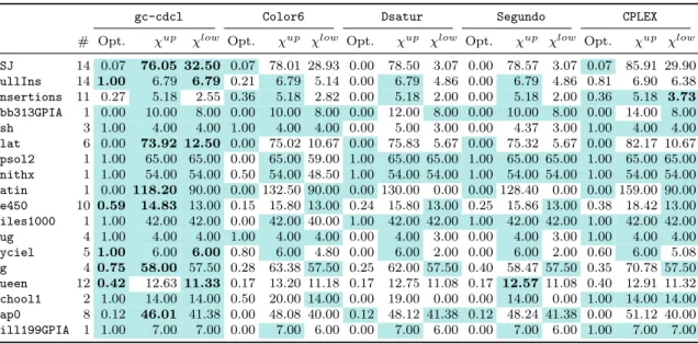
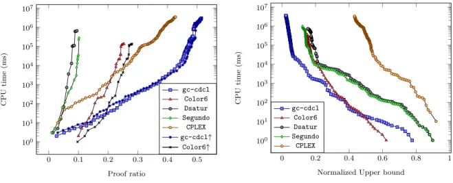
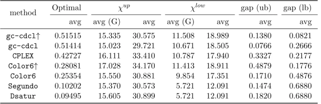
The combination of these techniques in both a branch-and-bound and in a bottom-up search outperforms other SAT-based approaches and Dsatur on standard benchmarks both for finding upper bounds and for proving lower bounds.
1. Introduction
Many applications require to partition items into a minimum number of subsets of compat-ible elements. For instance, when allocating frequencies, we may want to partition devices so that the physical distance between any two devices in a subset is large enough to share a frequency without interference (Aardal et al., 2007; Park & Lee, 1996). Alternatively, in compilers, we may want to partition frequently-accessed variables into registers so that two variables with overlapping live ranges are not given the same register (Chaitin et al., 1981). Many such combinatorial problems can be seen as a Graph Coloring Problem. The compatibility structure is represented by a graph G = (V, E) where V (the vertices) is a set of items and E (the edges) is a binary relation on V representing incompatibility. This problem is NP-hard, and in fact deciding if the chromatic number of a graph is lower than a given constant is one of Karp’s 21 NP-complete problems (Karp, 1972).
Although local search and meta heuristics can be extremely efficient for that problem, there are cases where proving optimality is important. For instance, in 2016, the U.S. Federal Communications Commission (FCC) conducted a reverse auction to acquire radio spectrum from TV broadcasters. At each iteration of the auction, the quote given by the FCC decrease and some potential sellers may opt out. The auction ends when it is not possible to allocate frequency bands (i.e., colors) to the broadcasters who opted out of the auctions (i.e., vertices) so that two broadcasters that can potentially interfere (i.e.,
adjacent) are allocated distinct frequency bands. This problem was solved by Newman et al. (2017) using a portfolio of mainly SAT-based solvers. Indeed, having a guarantee that the spectrum was acquired at the best price for the taxpayer was extremely important given the magnitude of the transaction.
Contributions. In this work1, we propose a novel approach to solving the vertex coloring problem. Our method is a hybrid of Conflict-Driven Clause Learning (Marques-Silva & Sakallah, 1999; Moskewicz et al., 2001) with techniques tailored to graph coloring. We use the idea of integrating constraint programming into clause learning satisfiability solvers by having each propagator label each pruning or failure by a clausal explanation (Katsirelos & Bacchus, 2005; Ohrimenko et al., 2007).
One of the main characteristics of the method we propose is to use a branching scheme proposed by Zykov (1949) whereby a choice point consists in either contracting two non-adjacent vertices, or adding an edge between them. This is not the first modern algorithm to use this technique. The branch and price algorithm proposed by Mehrotra and Trick (1995) branched using Zykov recurrence. Schaafsma et al. (2009) introduced edge variables, i.e. variables whose truth value indicates whether two vertices get the same color, in order to learn more general conflict clauses than the standard color-based SAT model permits. However, whereas the former method is based on an implicit exponential set of variables for computing a lower bound and the latter still requires standard variables standing for color assignment in order to branch and propagate, the method we propose relies entirely on edge variables.
There are two significant advantages to using Zykov recurrence. Firstly, color sym-metries are completely eliminated, at no significant computational cost. Secondly, when exploring a branch of the search tree, the density of the graph increases (through vertex contractions and edge additions) and computing a maximal clique of this graph gives an effective lower bound on the chromatic number.
Moreover, the use of a hybrid with constraint programming helps alleviate the potential drawbacks of this search scheme. Most importantly, edge variables can be made consistent at a reasonable computational cost via a dedicated propagator, whereas a clausal decom-position would be too costly and propagation using a partial coloring would be weaker. Moreover, it is possible to emulate Br´elaz’ Dsatur heuristic without maintaining a partial coloring, and experimental evaluation of the different approaches show that this is effective. The method we propose also uses a novel lower bound, stronger than cliques, based on finding a generalization of Mycielskian graphs (Mycielski, 1955) embedded in the current graph. Mycielskian graphs can have large chromatic number without necessarily containing large cliques. For example, the graphs M (k) described by Mycielski have chromatic number k and are triangle-free, i.e., they contain no clique of size 3. Therefore, the Mycielskian bound can potentially be stronger than the clique number. Since the two bounds (cliques and Mycielskians) rely on the same principle of isolating subgraphs with large chromatic number, failures have similar clausal explanations: at least one pair of vertices for which an edge was added must be contracted in order to find an improving coloring.
Then, we show how to detect vertex contractions or edge additions whose marginal cost with respect to either of these bounds violates the upper bound. In that case the domains
can be pruned accordingly. Thanks to this inference, our method is provably stronger than the standard branch and bound method in the sense that the search tree explored by the latter is larger.
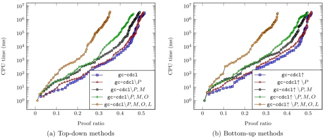
As a final contribution, we describe two additional new inference techniques. First we show how the propagation of learnt nogoods can be improved by taking into account the current state of the addition/contraction graph. This technique yields stronger, more general conflict clauses. Second, we introduce a preprocessing method whereby we extract an arbitrary independent set of the graph and replace it by constraints, thus yielding a model with fewer variables and which is stronger with respect to constraint propagation. These techniques can sometimes improve the performance of the proposed approach. In particular, the former significantly improves the results on two classes of benchmarks. However, on average over the whole data set we used, the impact is nearly null for the former and slightly negative for the latter.
2. Background
Graphs. A graph G is a pair (V, E) where V is a set of vertices and E is a set of edges. An edge is a binary set of distinct vertices, i.e., E ⊆ V2\ {(vv) | v ∈ V }. When (uv) ∈ E, we say that u and v are adjacent. We denote NG(v) the neighborhood {u | (uv) ∈ E} of v
in G (or N (v) when there is no ambiguity about the graph).
A coloring c of a graph is a labeling of its vertices such that adjacent vertices have distinct labels, and its cardinality is the total number of distinct labels. The chromatic number χ(G) of a graph G is the minimum cardinality of a coloring of G. The Graph Coloring Problem asks for a minimum coloring of a graph and the decision problem of whether there exists a coloring with at most k ≥ 3 colors is NP-complete.
A clique (independent set) is a set of vertices C ⊆ V , such that all pairs (no pairs) of vertices u, v of C are adjacent. The clique number (stability number) of a graph G, denoted ω(G) (α(G)), is the size of the largest clique (independent set) contained in G.
Since no two vertices in a clique can take the same color, we have ω(G) ≤ χ(G). Therefore, the size of a clique (maximum or not) can be used as lower bound. A coloring can be seen as a partition of a graph into independent sets (since no adjacent vertices may have the same color) and finding the optimum coloring is a set covering problem over all independent sets.
Constraint Satisfaction Problem. A constraint satisfaction problem is a triple (X, D, C) where X is a set of variables, D is the domain function and C is a set of con-straints. The domain function maps each variable X ∈ X to the set of its possible values. A (partial) assignment to X0 ⊆ X is a mapping from each X ∈ X0 to a value in D(X). A
complete assignment is a partial assignment to X. A constraint c is a pair (scope(c), Pc)
where scope(c) ⊆ X and Pc is a polynomial time predicate over assignments to scope(c).
A constraint is satisfied by an assignment A if Pc(A) is satisfied. A CSP is satisfied by a
complete assignment if every constraint c is satisfied by the restriction of that assignment to scope(c). Solving a CSP means finding a satisfying assignment and determining whether that exists is an NP-complete problem.
A value v ∈ D(X) is domain consistent (also called generalized arc consistent or GAC) with respect to a constraint C = (S, P ) with X ∈ S there exists an assignment A to S that
satisfies C and such that A(X) = v, otherwise it is domain inconsistent. A constraint is domain consistent if for all variables X ∈ scope(c) and all values v ∈ D(X), v is domain consistent with respect to c. A CSP is domain consistent if all its constraints are domain consistent. Domain consistency can be enforced by removing values from domains that are domain inconsistent, called pruning, until the unique domain consistent fixpoint is reached, or a constraint has no remaining satisfying assignments. Depending on the predicate of a constraint, the complexity of checking that a value is domain consistent may range anywhere from polynomial time to NP-complete.
CSP solvers that we care about in this paper solve an instance with backtracking search. Branching is typically binary, for example by assigning a variable to one of the values in its domain in one branch and removing that value in the other branch. Other schemes exist, but are not relevant to this work. At each node of the search, the solver executes a propagator for each constraint, which tightens the domains of the variables in its scope in order to enforce domain consistency, or potentially some weaker form of consistency. In the latter case, we say that the propagator is incomplete. Crucially for the success of constraint programming in general, propagators can execute any arbitrary algorithm, in particular algorithms that take advantage of domain knowledge and whose propagation cannot be replicated by simpler constraints (Bessiere et al., 2009).
Boolean Satisfiability. In satisfiability (SAT), we express problems with Boolean vari-ables X. We say that a literal l is either a variable x or its negation ¬x and we write x = var(l). Moreover, we write l = ¬l. Clauses are disjunctions of literals, written inter-changeably as sets of literals or as disjunctions, which are satisfied by an assignment if it assigns at least one literal to true. A formula is a conjunction of clauses, written also as a set of clauses and is satisfied by an assignment if it satisfies all clauses. The SAT problem is determining whether such a satisfying assignment exists and is NP-hard (Cook, 1971).
A SAT instance is closed under unit propagation if it contains no unit clauses. It is failed if it contains the empty clause. In order to compute the unit closure of an instance, for each unit clause (l) we remove all clauses that contain l and remove l from other clauses. We call this procedure performing unit propagation.
The state of the art in solving SAT is the Conflict-Driven Clause Learning (CDCL) algorithm (Marques-Silva & Sakallah, 1999; Moskewicz et al., 2001). The basic techniques used in CDCL are a variant of backtracking search with unit propagation at each node, frequent restarting and far-backjumping, learning implied constraints from conflicts in the backtracking search which empower unit propagation (clause learning) and activity based branching (VSIDS).
The techniques of CDCL can be readily adapted in CSP solvers, except for clause learning. It has been shown (Katsirelos & Bacchus, 2005) that it is possible to do this as well by using an appropriate propositional encoding of domains and generating clausal explanations for each pruning and each constraint failure. This can be further improved for some highly useful classes of constraints by using a domain encoding that takes domain order into account (Ohrimenko et al., 2007). We shall abuse CSP notations when considering Boolean literals. In particular, for a constraint involving a Boolean variable x, we shall say that x (resp. ¬x) is GAC if and only if the assignment x = 1 (resp. x = 0) is GAC.
3. Related Work
Complete approaches for the graph coloring problem can be broadly divided into three categories: branch and bound, branch and price, and satisfiability-based.
Branch & Bound. One of the oldest and most successful techniques is a backtracking algorithm using Br´elaz’ Dsatur heuristic (Br´elaz, 1979): when branching, the vertex with highest degree of saturation is chosen and colored with the lexicographically least candidate. The degree of saturation of a vertex v is the number of assigned colors within its neighbor-hood N (v) in G. In case of a tie, the vertex with largest number of uncolored neighbors is chosen among the tied vertices. This heuristic is often used within a branch-and-bound al-gorithm with one variable per vertex whose domain is the set of possible colors. It is known as dom+deg in the CSP literature (Frost & Dechter, 1995). More sophisticated tie-breaking heuristics have been shown to improve Dsatur (Segundo, 2012).
One common caveat of Dsatur-based branch and bound algorithms, however, is that the standard lower bound, which is the size of a maximal (not necessarily maximum) clique, is computed only once at the root of the search tree. Indeed, the algorithm branches on the coloring, but the structure of the graph does not change, hence there is no point in computing another clique. Consequently, Furini et al. (2016) proposed three lower bound techniques taking advantage of the coloring decisions. The first introduces an auxiliary graph where the vertices sharing the same color are merged on which cliques are easier to compute and are potentially larger. The second relies on computing the Lov´asz Theta number (Lov´asz, 1979), which lies between the clique number and chromatic number of a graph (Gr¨otschel et al., 1981) and which can be computed in polynomial time using semi-definite programming. Finally, the third bound uses a different auxiliary graph whose independent sets can be mapped to coloring of the original graph (Cornaz & Jost, 2008). Branch and price. A second type of approaches rely on the column generation method (Mehrotra & Trick, 1995; Malaguti et al., 2011). The problem is a seen as a set covering problem over all independent sets of the graph which are the 0-1 variables of the integer linear program. Independent sets, however, are dynamically generated and when no inde-pendent set that can potentially improve the master problem can be found, the current solution of the set covering is an optimal coloring. This method is significantly better than Dsatur-based approaches on some classes of graphs, however, it can be significantly outperformed on some other classes (Malaguti & Toth, 2010; Segundo, 2012).
Boolean Satisfiability. A third type of approaches rely on Boolean Satisfiability. In order to encode graph coloring with satisfiability, some approaches rely on color variables xvi, where xvibeing true means vertex v takes color i. For every edge (uv), there is a binary
clause xvi∨ xui for every color i. If k is the maximum number of colors, then there is a
clauseW
1≤i≤kxui. This corresponds to the direct encoding (Walsh, 2000) of the constraint
model where we have a color variable Xv for each vertex v, whose domain ranges from
1 to k and which indicates its assigned color and a constraint Xv 6= Xu for all pairs of
adjacent vertices. The CP and SAT models are exactly identical, so we refer to both by the same name. Refinements to this encoding include Van Gelder’s log encoding versions, where xvj is true if the j-th bit of the binary encoding of the color taken by vertex v is
(Gomes et al., 1998; Huang, 2007) and clause learning (Marques-Silva & Sakallah, 1999) are not straightforward to combine with symmetry breaking such as that of Van Hentenryck et al. (2003) since it relies on dedicated branching. They can only be easily combined with starting from an arbitrary coloring to a clique, but that is incomplete. The Color6 solver (Zhou et al., 2014) uses symmetry breaking branching but forgoes restarting to maintain complete symmetry breaking.
Zykov’s recurrence. In contrast to branching on colors, the search tree induced by the recurrence relation (1) below, due to Zykov (1949), has no color symmetry.
Let G/(uv) be the graph obtained by contracting u and v: the two vertices are removed and replaced by a single new vertex r(u) = r(v) and every edge (vw) or (uw) is replaced by (r(v)w). Conversely, let G + (uv) be the graph obtained by adding the edge (uv), in which case we say that the vertices are separated.
χ(G) = min{χ(G/(uv)), χ(G + (uv))} (1)
Indeed, given a coloring of G, either the vertices u and v have distinct colors hence it is also a coloring of G + (uv), or they have the same color and it is a coloring of G/(uv).
Moreover, branching using this recurrence yields graphs with non-decreasing sets of edges. Therefore, using the clique number as lower bound is easy, and this lower bound can only increase when branching. In contrast, in the color variable formulation, the standard technique is to compute a clique at the root node only as discussed earlier.
Example 1. Figure 1 illustrates the Zykov recurrence. From the graph G in Figure 1a, we obtain the graph G + (cd) shown in Figure 1b by adding the edge (cd) and the graph G/(cd) shown in Figure 1c. One of these two graphs has the same chromatic number as G.
a b c d e f g (a) G a b c d e f g (b) G + (cd) a b c, d e f g (c) G/(cd)
Figure 1: Zykov recurrence
This branching scheme was successfully used in a branch-and-price approach to color-ing (Mehrotra & Trick, 1996). In the context of satisfiability, Schaafsma et al. (2009) introduced a novel and clever way of taking advantage of Zykov’s idea: first, they intro-duce edge variables for every pair of non-adjacent vertices. When an edge variable is set to true, the two vertices get the same color, and are assigned different colors otherwise. Then, when learning a clause involving color variables, they show that one can compactly encode all symmetric clauses using a single clause that only uses edge variables and propagates
the same as if all the symmetric clauses were present. In their approach, they only intro-duce edge variables as needed and they have no lower bound computation except for that achieved by attempting to assign the color variables. They achieve good empirical results, but the scheme is quite complicated to implement.
4. Zykov Tree Search
In our approach, similar to that of Schaafsma et al., we use a model which leads to the exploration of the tree resulting from the Zykov recurrence. We have one Boolean edge variable euv for each non-edge of the input graph with the same semantics as those used for
edge variables by Schaafsma et al. A complete assignment partitions the vertices of G into a set of independent sets, which correspond to colors. The number of independent sets is the size of the coloring that we have computed. We somewhat abuse notation in the sequel and write clauses using variables euv even when (uv) ∈ E and assume that the variable is
always false. Moreover, in this paper we consider only undirected graphs, hence euv and
evu are the same variable.
The decision to assign the same color to two vertices is the same as following the branch that contracts the vertices in the Zykov recurrence, while assigning them different colors corresponds to the branch that adds an edge between them. Therefore, we can associate a graph GX with a (partially assigned) set of edge variables X. GX is the graph that results
from contracting all vertices u, v of G for which euv is true and separating (adding an edge
between) all pairs of vertices u, v of G for which euv is false. When euv and evw are both
true, this means that we contract u and v and then contract w and r(v). Similarly, if euv
is true and evw is false, we contract u and v and add an edge between r(v) and w. The
operation of contracting vertices is associative and commutative, so we get the same graph GX regardless of the order in which we process the variables in X. It is also a bijection, so
each contracted graph can be mapped back to exactly one assignment. We can therefore use X and GX interchangeably.
We now describe a propagation algorithm for the following constraint Coloring, for a graph G = (V, E), an integer k, and the set of variables X = {euv| u, v ∈ V }:
Coloring(G, k, X) ≡ ∃c : V 7→ N c(u) = c(v) =⇒ euv
∧ |{c(u) | u ∈ V }| ≤ k ∧ (2)
euu ∀u ∈ V ∧ (3)
euv ∀(uv) ∈ E (4)
The constraint Coloring is satisfied by any assignment of the edge variables that cor-responds to a coloring with fewer than k colors, and is therefore clearly NP-hard. Equation 2 enforces that the equalities are consistent with a k-coloring, while constraints 3 and 4 ensure that the coloring is legal with respect to the edges of the graph.
Moreover, the property of having the same color is transitive, so if euv and evw are true,
then so is euw. Transitivity also implies that if euv is true and evw is false, then euw must
also be false. We enforce transitivity using the implied constraint Transitivity:
We can enforce GAC on this constraint using a clausal decomposition of size O(|V |3):
(euv∨ evw∨ euw) ∀u, v, w ∈ V (6)
Performing unit propagation on this decomposition takes O(|V |3) time cumulatively over a branch of the search tree. In our implementation, we have opted instead for a dedicated propagator described in Section 4.2, whose complexity over a branch is only O(|V |2).
Let |GX| be the number of vertices of the graph GX resulting from the additions and
contractions X. From Zykov (1949), we know that there exists a transitive assignment of X, compatible with the edges of G such that |GX| = χ(G) (and trivially, |GX| ≥ χ(G) for
any X). Therefore, the constraint Coloring can be rewritten: Coloring(G, k, X) ≡ Transitivity(G, X) ∧
|GX| ≤ k ∧
euu, ∀u ∈ V ∧
euv, ∀(uv) ∈ E
We describe two algorithms for computing lower bounds on |GX| in Sections 5.1 and
5.2. The first algorithm computes the well known clique lower bound (Section 5.1) on the graph GX and the second a novel, stronger, bound (Section 5.2). If that bound meets or
exceeds k, the propagator fails and produces an explanation. Moreover, we describe how to (incompletely) prune the domains of with respect to these bounds in Section 6.3.
Neither of the bounds that we use is cheap to compute, and computing marginal costs in order to prune domains can be expensive as well, hence the propagator for the bound runs at a lower priority than unit propagation and the Transitivity constraint.
Clearly, our approach is closely related to that of Schaafsma et al. However, there are some important differences. First, since we do not need the color variables to compute the size of the coloring, we completely eliminate the need for the clause rewriting scheme that they implement and get color symmetry-free search with no additional effort. In addition, since our model is a CP/SAT hybrid model, we can use a constraint to compute a lower bound at each node, thus avoiding a potentially large number of conflicts.
The approach of Schaafsma et al. of decomposing the constraint Transitivity using color variables (so that Xv = Xu ⇐⇒ euv) does not enforce domain consistency on the
constraint Transitivity. For instance, consider three vertices u, v and w such that Xv, Xu
and Xw can all take values in {1, 2} and we have the unit literals euv and euw. The literal
evw is not GAC for Transitivity, however it is GAC for the decomposition. In contrast,
the propagator described in Section 4.2 maintains GAC on this constraint, without having to encode channeling between the edge variables and the color variables.
The main drawback of this model is that we need a large number of variables. This is especially problematic for large, sparse graphs, where the number of non-edges is quadratic in the number of vertices and significantly larger than the number of edges. Indeed, in 4 of the 125 instances we used in our experimental evaluation, our solver exceeded the memory limit2. The approach of Schaafsma et al. does not have the same limitation, as
they introduce variables only when they are needed to rewrite a learnt clause, in a way similar to lazy model expansion (De Cat et al., 2015). It is possible that this approach of lazily introducing variables can be adapted to our model, but this, as well as other ways of reducing the memory requirements, remains future work.
4.1 Optimization Strategy
Previous satisfiability-based approaches to coloring have mostly ignored the optimization problem of finding an optimal coloring of a graph and instead attack the decision problem of whether a graph is colorable with k colors. In our setting, we have the flexibility to do both. In particular, before starting search the solver computes initial bounds χlow ≤ χ ≤ χup for
the chromatic number, using the bound described in section 5.1 or 5.2 and a run of the Dsatur heuristic, respectively.
After that, it may use one of two search strategies: branch-and-bound or bottom-up. The former uses a single instance of a solver, uses χup to create the initial Coloring constraint and then iteratively finds improving solutions. For each solution, it adds to the model a new Coloring constraint with the new, tighter, upper bound3. This is similar to the top-down approach one would use when solving a series of decision problems, starting from a heuristic upper bound and decreasing that until we generate an unsatisfiable instance, in which case we have identified the optimum. The advantage of the branch-and-bound approach is that it does not discard accumulated information between solutions, namely learned clauses and heuristic scores for variables. Moreover, it more closely resembles the typical approach used in constraint programming systems.
The bottom-up approach temporarily sets χup = χlow and tries to solve the resulting instance, i.e., one in which k = χupin the Coloring constraint. If the instance is satisfiable, it terminates with χ = χlow, otherwise it increases χlow by one and iterates until the lower bound meets the true chromatic number. This has none of the advantages of the branch-and-bound approach, as it is not safe to reuse clauses from a more constrained problem in one that is less constrained. Moreover, it cannot generate upper bounds before it finds the optimum. But it gains from the fact that the more constrained problems it solves may be easier. One particular behavior we have observed is that sometimes the lower bound computed at the root coincides with the optimum and finding the matching upper bound is quite easy with the bottom-up strategy, while finding that solution with branch-and-bound can be very hard.
4.2 Transitivity Propagation
The propagator for the Transitivity (G, X) constraint works by maintaining a graph H that is updated to be equal GX as the current partial assignment A grows and using that
to compute the literals that must be propagated. For brevity, in the rest of this section, we always write N (v) to mean NH(v) and abuse the neighborhood notation to write N (S) for
S
u∈SN (u). Additionally, the propagator maintains for each vertex v a bag b(v) to which
it belongs. Each unique bag corresponds to a vertex in H. Initially, b(v) = {v} for all v, since no contractions have taken place.
3. The actual implementation makes this modification in-place so that the number of Coloring constraints remains 1, regardless of the number of solutions found.
We set the propagator for Transitivity (G, X) to be invoked for every literal that becomes true. Call this literal p. When the propagator is invoked for p = euv, which
corresponds to the contraction of u and v, then all vertices v0 ∈ b(v) and u ∈ b(u) must be assigned the same color, so it sets eu0v0 to true for all v0 ∈ b(v), u0 ∈ b(u). The contraction
implies that every vertex in b(v) must be separated from all vertices in N (b(u)) with which it does not already have an edge (and symmetrically for vertices in b(u)). Hence the propagator also sets eu0v0 to false for all v0 ∈ b(v) and u0 ∈ N (b(u) \ N (b(v)) and for all v0 ∈ N (b(v) \
N (b(u)). Finally, it sets B = b(u) ∪ b(v), updates b(v0) = B for all v0 ∈ B and contracts v and u in H. In the case where the propagator is invoked for p = euv, it sets eu0v0 to false
for all v0 ∈ b(v), u0 ∈ b(u) and adds an edge between v and u in H.
A small but important optimization is that if the propagator is invoked for euvbecoming
true (resp. false) but u and v are already in the same bag (resp. already separated) then it does nothing. This ensures that it touches each non-edge at most once, hence its complexity is quadratic over an entire branch. This is also optimal, since in the worst case every variable must be set either as a decision or by propagation. Notice also that the operation of merging and keeping track of b(v) can be performed in amortized constant time using the union-find data structure (Tarjan & van Leeuwen, 1984), where euvbecoming
true entails the union operation Union(v, u) and r(v) = Find(v). Of the two, the latter is important, as we can check whether two vertices v, u have been contracted by checking whether Find(v) = Find(u), or r(v) = r(u). On the other hand, amortized constant time Union is not important, because contracting two vertices u, v has complexity O(|b(v)||b(u)|), which dominates even a naive implementation of Find. Indeed, since the algorithm has to iterate over all vertices in both bags anyway, our implementation simply updates r(u) as it performs this iteration.
This propagator uses the clauses (6) as explanations. The way it chooses explanations for literals that it propagates is fairly straightforward, using the vertices involved in the literal that woke the propagator as pivots. For example, if b(v) = {v, v0}, b(u) = {u, u0} and it is woken on the literal euv, it sets euv0 using (evv0 ∨ euv∨ euv0) as the reason, eu0v using
(euu0∨ euv∨ eu0v), and only then finally setting eu0v0 using (euv0 ∨ euu0∨ eu0v0) which relies
on the fact that euv0 has been just set to true.
4.3 Transitivity-Aware Unit Propagation
Consider a (learned) clause c = (F ∨ evu∨ evw), where F is a set of literals which are all
false in the current node of the search tree and u, w are in the same bag. Notice that if we set evw to false, the transitivity propagator will also set evu to false, since v and w are
in the same bag. This will violate clause c and hence we should set both evw and evu to
true. More generally, when c = (F ∨ B), all the literals in F are false, and B are the only unset literals, they have the same polarity and are over vertices that belong to exactly two bags, the literals in B will all necessarily get the same value: we will either merge the two bags, so all variables become true, or we will add an edge between them and all variables become false. So if the unset literals are negative, we must satisfy them all by adding an edge between the bags, while if they are positive, we must satisfy them all by merging the two bags.
Unit propagation is unable to make any inference when more than one literal is unset, while the transitivity constraint is unaware of the learned clauses, so this inference cannot be made by any single component of the solver. In order to detect this situation, the unit propagation procedure can be made aware of vertices and partitions. In particular, suppose we have a clause c, watched by l1 with var(l1) = euv and l2, and l2 has just become false.
The standard unit propagation algorithm finds another, non-false, literal l3 6= l1 and uses it
as the watch, or determines that the clause is unit or failed if no such literal exists. Instead of stopping on the first non-false literal, we keep on searching for a literal l3 that is either
a) true, b) has different polarity to l1 or c) var(l3) = ewz and {r(u), r(v)} 6= {r(w), r(z)},
i.e., u and v are not assigned to exactly the same partitions as w and z. If any of these conditions is true, we use l3 as the new watch and continue. If not, then the clause has been
reduced to a positive or negative clause over variables involving exactly two partitions and hence other literals must either all be true or all false because of the transitivity constraint. Since the clause must be satisfied, we must make one of them true.
We cannot use the clause c as the reason for this propagation, since it is not unit. To construct an explanation, let l be the literal that we have chosen to make true, with var(l) = euv, and let VB be the vertices {v | l0 ∈ B ∧ var(l0) = euv}. In other words, the set
B is the set of vertices which appear as a subscript of a literal euv or euv in B. Partition
VB into V1 and V2 such that V1 = {w | w ∈ VB∧ r(w) = r(v)} and V2 = Vb\ V1. Then, the
explanation is F ∪ {l} ∪ {euu0 | u0 ∈ V1\ {u}} ∪ {evv0 | v0 ∈ V2\ {v}}. In words, the clause
states that because all literals in F are false, the vertices in V1 are in the same bag as u,
and the vertices in V2 are in the same bag as v, we must make l true.
Example 2. Consider again the clause c = (F ∨ evu ∨ evw) where all literals in F are
false, evu and evw are unset and u, w are in the same bag. Since this clause meets the
conditions defined above, we can make the literal l = evw true. Since the clause c has two
unset literals, it cannot be used as the clausal explanation for setting l to true. To construct the explanation, we proceed as above with B = {evu, evw}, VB= {v, u, w} and partition this
into V1 = {u, w} and V2= {v}. The clausal explanation we compute is F ∪ {evw} ∪ {euw}.
To see why this a valid explanation, consider the case where the literal l is positive, i.e., l = evu. We trace back the steps that propagation of the Transitivity constraint would
perform if we set l to false. For each literal l0 ∈ B, l0 = ev0u0, l 6= l0, u0 ∈ V1, v0 ∈ V2, we
resolve with the clauses {euu0, eu0v, euv} and {evv0, eu0v0, eu0v}, both of which are entailed by
the Transitivity constraint. This eliminates the literal eu0v0, introduces euu0 and evv0 as
required and leaves euv in the clause. Once we repeat this for all literals l0 6= l, l0 ∈ B, we
get the explanation clause described above. Similar reasoning can be used when v = v0 or u = u0 and for the case where l is negative.
This feature makes unit propagation stronger at a moderate increase in runtime cost. In our experiments in Section 7, we show that while using this technique does not pay off overall, it improves performance in some classes.
4.4 Emulating Br´elaz Heuristic in Zykov Search Tree
Schaafsma et al. have already shown that any particular partial coloring can be mapped to a node in the Zykov recurrence. We have alluded to the procedure for doing this earlier: we contract all vertices that get the same color and add edges between vertices that get
different colors. The correspondence also works in the other direction, although it is not unique: from every node of the Zykov recurrence, we can construct several possible partial colorings. Consider a node n of the Zykov recurrence and the graph Gn at that node.
We can choose any maximal clique in Gn and color its vertices arbitrarily to get a partial
coloring. Since there are (exponentially) many cliques in a graph, this is clearly not a unique mapping. However, it allows us to replicate in the Zykov model any computation that requires a coloring to work with.
In particular, Br´elaz’ branching heuristic remains extremely competitive for finding good colorings, as evidenced by the performance of the Dsatur method in our experimental eval-uation (Section 7). Moreover, Schaafsma et al. observed that branching on color variables was significantly better than branching on edge variables. We therefore use the observation above to emulate this heuristic without introducing color variables.
Indeed, adding color variables is not really desirable. First, it adds the overhead of propagating the reified equality constraints. Second, using these variables to follow Dsatur requires branching on them, which in turn requires some kind of symmetry breaking method, like the rewriting scheme of Schaafsma et al. So it would be preferable to get the benefit of the more effective branching heuristic without needing to introduce color variables.
As shown earlier, we can achieve behavior similar to that of Dsatur in the edge variable model, by exploiting the mapping from the current graph GX back to a coloring of the
original graph. To do this, we pick a maximal clique C in GX. We pick the vertex v
that maximizes |N (v) ∩ C|, breaking ties by highest |N (v) \ C|, and an arbitrary vertex u ∈ C \ N (v). Notice that u may not exist when the original graph is not connected. In this case we pick a different clique until we find a clique C with N (v) ∩ C 6= ∅. We then set euv
to true. This uses the current maximal clique to implicitly construct a coloring and uses that to choose the next vertex to color as Dsatur does. If the assignments euv are refuted
for all u ∈ C, then v is adjacent to all vertices in C and so C ∪ {v} is a larger clique, which corresponds to using a new color in Br´elaz’ heuristic. This construction generalizes the construction we discussed earlier. From a node of the Zykov recurrence, we can construct not only a coloring, but also the state of the domains in the color variable model under that coloring, so that, for example, the current domain size of Xv is χup− |N (v) ∩ C|.
This branching strategy can be more flexible than committing to a coloring by assigning the color variables. For example, unit propagation on learned clauses as we explore a branch of the search tree can make it so that the maximal clique C0 at some deep level is not an extension of the maximal clique C at the root of the tree, i.e., C 6⊆ C0. This is further supported by our experiments juxtaposing the two algorithms for finding cliques that we describe in Section 5.1: the one that tries to extend a clique performs overall worse than the computationally more costly algorithm which non-incrementally searches for cliques in the entire graph. The Br´elaz heuristic on the color variables commits to using C at the root, hence cannot take advantage of the information that C0 is a larger clique. The modification that we present here achieves this.
5. Lower Bounds
As we already discussed, an important advantage of the edge-variable based model is that computing a lower bound for the current subproblem is as easy as for the entire problem.
For example, for X the set of partially assigned edge variables, the clique number of the graph GX is a lower bound for the subproblem.
5.1 Clique-Based Lower Bound
In order to find a large clique we use the following greedy algorithm, called GreedyCliqueFinder. Let o be an ordering of the vertices, so we visit all vertices in the order vo1, . . . , von. We maintain an initially empty list of cliques. Iterating over all vertices
in the order o, we add each vertex to all the cliques which admit it and if no clique admits it we put it in a new singleton clique. When this finishes, we iterate over the vertices one more time and add them to all cliques which admit them, because in the first pass a vertex v was not evaluated against cliques which were created after we processed v. We then pick the largest among these cliques as our lower bound.
The number of bitwise operations performed by this algorithm is O(|V |2). Indeed, we construct at most |V | cliques and for each vertex we check whether it can be added to each clique. The bitwise operations each have cost O(|V |), so the complexity of the algorithm is O(|V |3), but we found it practical to think in terms of number of bitwise operations, as their cost if often near-constant time, at least for the graph sizes we dealt with.
We tried a few different heuristics for the ordering o of the vertices, including the in-verse of the degeneracy order (Lick & White, 1970), which tends to produce large cliques (Eppstein et al., 2013; Jiang et al., 2017). We found that it works best to sort the vertices in order of decreasing bag size.
If the lower bound meets or exceeds the upper bound k, the propagator reports a conflict. We construct a clausal conflict as follows: each vertex v of the current graph is the result of the contraction of one or more vertices of the original graph. In keeping with the notation for the transitivity propagator, we call this the bag b(v). We arbitrarily pick one vertex r(v) from the bag of each vertex v in the largest clique C, and set the explanation to
_
v,u∈C
er(v)r(u) (7)
This clause contains O(|C|2) positive literals. When we falsify it, it means that the corresponding contracted graph contains edges between all pairs of vertices in C. Therefore, falsifying the clause entails violating the upper bound, so it is logically entailed.
This explanation is not unique. In particular, we can generate mixed-sign clauses as explanations, which are also shorter.
Example 3. Suppose that under the current partial assignment to X, the graph GX contains
the clique C = {v, u1, u2, w1, w2} such that v corresponds to the bag {u, w} and |C| ≥ χup.
Further suppose that NG(u) = {u1, u2} and NG(w) = {w1, w2}. To generate an explanation
for this according to (7) we arbitrarily pick r(v) = u and the clause that we generate will be of the form c ∪ {euw1, euw2}, where c contains the literals implied by (7) which involve only
the vertices {u1, u2, w1, w2}. It also implicitly includes the literals {euu1, euu2}, but since
the edges (u, u1) and (u, u2) are present in G, it is as if there exist unit clauses (euu1) and
(euu2), so they can be resolved away from the explanation clause. However, this clause is
falsifying it means that we make euw true, which means that we contract u and w and that
the resulting vertex has neighborhood {u1, u2, w1, w2}. Moreover, this clause that contains
both positive and negative literals is shorter than the clause generated by (7) by 1 literal, because the single contraction entails 4 edge additions ((u, w1), (u, w2), (w, u1), (w, u2)), two
of which ((u, w1), (u, w2)) are needed for the explanation.
This example can be extended to show that in some cases it is possible to generate an explanation of length O(|C|) as opposed to O(|C|2). We have experimented with producing such mixed-sign explanations. However, it is computationally costly to find which choice of representative from each bag generates the shortest clause. Moreover, although mixed-sign explanations that we tried tend to be much shorter and speed up search in terms of number of conflicts per second, they also significantly increase the overall effort required, both in number of conflicts and runtime. Therefore, we use exclusively the positive clauses given by equation (7).
Incremental clique updates. The heuristic method we described above for finding cliques has the disadvantage that it examines the entire (contracted) graph each time that the propagator is invoked. Depending on the instance, this can end up a significant over-head. Therefore, we have also implemented a different method which sacrifices the quality of the bound to achieve significantly better performance per invocation.
This algorithm, which we call IncrementalCliqueFinder, proceeds as follows. When invoked at the root of the tree, it only forwards to GreedyCliqueFinder and then discards all cliques except those that have largest cardinality. For subsequent invocations, it requires access to a list of vertices which have gained edges as a result of contraction or separation of vertices in the graph. When we contract u and v as a result of euv becoming true,
both vertices may gain new edges, as their neighborhoods are updated to all be identical N (v) ∪ N (u). Similarly, when we separate two vertices which were previously non-neighbors as a result of evu becoming false, both u and v gain an edge in their neighborhood. The
neighborhood of all such vertices may now contain one of the cliques which we have stored (but when we contract two vertices v, u, only r(v) = r(u) is examined). This list can be easily kept up to date as the propagator is woken for every literal that becomes true or false. Given this list, IncrementalCliqueFinder examines each vertex v in it and adds v to all stored cliques C such that N (v) ⊇ C. At the end, it again filters the set of stored cliques to keep only those with largest cardinality. IncrementalCliqueFinder returns this largest cardinality as the lower bound.
One complication is that on backtracking, the set of stored subgraphs are no longer cliques, as vertices are uncontracted and edges removed, hence they are invalid. Rather than implement a trailing or copying scheme for these cliques, after a conflict IncrementalCliqueFinder again simply forwards to GreedyCliqueFinder, as it does at the root.
The advantage of IncrementalCliqueFinder, compared to GreedyCliqueFinder, is that it examines only the part of the graph that has been modified since the last invocation, and that only in relation to a small set of cliques. More concretely, if the neighborhood of p vertices has changed and it has stored q cliques, it performs O(pq) bitwise operations to update the set of cliques and get a new bound, so its complexity is O(pq|V |). Empirically, q is small (less than 5), so even if nearly all vertices have had their neighborhood changed,
it is faster than GreedyCliqueFinder by a factor of |V | and even faster in the more typical case where only a small subset of vertices have changed since the last invocation.
Despite the advantage of IncrementalCliqueFinder over GreedyCliqueFinder in terms of runtime complexity, we have discovered empirically that the cliques that cause bound violations may arise from regions of the graph that initially do not contain large cliques and will therefore be ignored by IncrementalCliqueFinder. This is somewhat mitigated by the fact that we store all cliques of largest cardinality and that we call GreedyCliqueFinder after every conflict. However, as we show in Section 7, using the IncrementalCliqueFinder algorithm in our solver degrades overall performance, despite the fact that it improves speed in terms of number of conflicts per second.
The empirical observation that finding diverse sets of cliques is important for perfor-mance is also informative in light of the correspondence between nodes of the Zykov tree and colorings of the graph, discussed in Section 4. Since a) finding diverse sets of cliques is important for performance, b) maintaining a single coloring is analogous to maintaining a single clique, and c) using color variables forces us to maintain a single coloring, we conclude that using color variables cannot replicate the results of using edge variables.
5.2 Mycielski-Based Bound
Although being a useful bound in practice, the clique number is both hard to compute and gives no guarantees on the quality of the bound. We propose here a new lower bound inspired by Mycielskian graph.
Definition 1 (Mycielskian graph (Mycielski, 1955)). The Mycielskian graph µ(G)=(µ(V ),µ(E)) of G =(V ,E) is defined as follows:
• µ(V ) contains every vertex in V , and |V | + 1 additional vertices, the vertices U = {ui | vi ∈ V } and another distinct vertex w.
• For every edge vivj ∈ E, µ(E) contains vivj, viuj and uivj. Moreover, it contains all
the edges between U and w.
The Mycielskian µ(G) of a graph G has the same clique number, however its chromatic number is χ(G) + 1. Indeed, consider a coloring of µ(G). For any vertex vi ∈ V , we have
N (vi) ⊆ N (ui), and therefore we can safely use the same color vi as for ui. If can be shown
that at least χ(G) colors are required for the vertices in U , and since N (w) = U , then w requires a χ(G) + 1-th color. Mycielski introduced these graphs to demonstrate that triangle-free graphs can have arbitrarily large chromatic numbers, hence the clique number does not approximate the chromatic number.
The principle of our bound is a greedy procedure that can discover embedded pseudo Mycielskians. Indeed, the class of embedded graphs that we look for is significantly broader than the set of pure Mycielskians {M2, M3, M4, . . .}. First, the witness subgraph may not
necessarily be induced. Therefore, trivially, Mycielskians with extra edges also provide valid lower bounds. Moreover, rather than starting from a single edge, as in the construction of the pure Mycielskians, we construct Mycielskians of cliques. Finally, the method we propose can also find Mycielskians modulo some vertex contractions. Clearly, those are also valid lower bounds since contracting vertices is equivalent to adding equality constraints to the problem.
(a) M2 (b) M3 (c) M4
Figure 2: A 2-clique M2 = µ(∅), its Mycielskians M3= µ(M2) and M4 = µ(M3)
Given a subgraph H = (VH, EH) of G, and v ∈ VH, we define:
Sv = {u | NH(v) ⊆ NG(u)} (8)
Suppose that there exists a vertex w with at least one neighbor in every set Sv:
w ∈ ∩v∈VHNG(Sv) (9)
and let u(v) be any element of Sv such that u(v) ∈ NG(w) and U = {u(v) | v ∈ V }, then:
Lemma 1. H0 = (V ∪ U ∪ {w}, E ∪ [ v∈V NH(v) × u(v) ∪ [ u∈U {(uw)}) =⇒ χ(H0) ≥ χ(H) + 1
Proof. The proof follows from the facts that H0 is the Mycielskian graph of H possibly with contracted vertices, and is embedded in G.
Suppose first that, for each v ∈ V , u(v) 6= v and w 6∈ V . Then we have H0 = µ(H) by using u(vi) for the vertex ui, and w for itself, in Definition 1.
Suppose now that H0 6= µ(H). This can only be because either:
• For some vertex vi of H, we have u(vi) = vi. In this case, consider the graph µ(H)
and contract ui and vi. The resulting graph µ(H)/(uivi) has a chromatic number at
least as high as µ(H). However, it is isomorphic to H0.
• The vertex w is the vertex vi from the original subgraph H. Here again contracting vi and w in µ(H) yields H0.
Notice that there is not a third case where w is taken among U since, for any v ∈ VH,
we have u(v) 6∈ ∩v∈VHNG(Sv) because u(v) is not a neighbor of itself.
Example 4. Figure 3a shows the graph G/(cd) obtained by contracting vertices c and d in the graph G of Figure 1. Let H be the clique {a, b, c}. We have Sa = {a, e}, Sb = {b, f }
and Sc = {c}. Furthermore, NG({a, e}) ∩ NG({b, f }) ∩ NG({c}) = {b, c, g} ∩ {a, e, c, g} ∩
{a, b, e, g, f } = {g}, from which we can conclude that this graph has chromatic number at least 4. As shown in Figure 3b, when called with H = {a, b, c} Algorithm 1 will extend it with a first layer U = {e, c, f } and an extra vertex w = g. Notice that the graph obtained by adding the edge (cd) has a 4-clique (see Figure 1). Therefore, the graph G in Figure 1a also has a chromatic number of at least 4.
a b c, d e f g (a) H = G/(cd) a b c, d u(a) u(b) w (b) Trace of Algorithm 1 on H
Figure 3: Embedded Mycielski
Algorithm 1 greedily extends a subgraph H = (VH, EH) of the graph G (with χ(H) ≥ k)
into a larger subgraph H0 = (VH0 , EH0 ), following the above principles. As long as this succeeds, in the outermost loop, we replace H by H0 and iterate. The computed bound k is equal to χ(H) plus the number of successful iterations.
We compute the sets Sv (Equation 8) and the set W of nodes with at least one neighbor
in every Sv in Loop 1. Then, if it is possible to extend H (Line 4), we compute the pseudo
Mycielskian (VH0 , EH0 ) as shown in Lemma 1 and replaces H with it in Line 5 before starting another iteration.
Complexity. An iteration of Algorithm 1 does O(|VH| × |V |) bitset operations (Line 2 is
1 ‘AND’ operation and Line 3 is O(|V |) ‘OR’ operations and 1 ‘AND’). The second part of the loop, starting at Line 4, runs in O(|VH|2) time. Typically, the number of iterations
is very small. It cannot be larger than log |V | since the number of vertices in H is (more than) doubled at each iteration. It follows that Loop 1 is executed at most 2|V | times, and therefore, the worst case time complexity is O(|V |2) bitset operations (hence O(|V |3) time).
Explanation. Similarly to the clique based lower bound, the explanations that we pro-duce here correspond to the set of all edges in the graph H:
_
(uv)∈EH
euv (10)
Adaptive application of the Mycielskian bound. In preliminary experiments, we found that trying to find a Mycielskian subgraph in every node of the search tree was
Algorithm 1: MycielskiBound(k, H = (VH, EH), G = (V, E)) while |VH| < |V | do W ← V ; ∀v ∈ VH Sv ← {v}; 1 foreach v ∈ VH do foreach u ∈ V do
2 if NH(v) ⊆ NG(u) then Sv← Sv∪ {u} ;
3 W ← W ∩ NG(Sv); 4 if W 6= ∅ then k ← k + 1; (VH0 , EH0 ) ← (VH, EH); w ← any element of W ; foreach v ∈ VH do VH0 ← VH0 ∪ { any element of (NG(w) ∩ Sv)}; EH0 ← E0H∪ {(wu)} ∪ {u × NH(v)}; 5 (VH, EH) ← (VH0, EH0 ); else break; return k;
too expensive and did not pay off in terms of total runtime. Therefore, we adapted a heuristic proposed by Stergiou (2008) which allows us to apply this stronger reasoning less often. In particular, we only compute the clique lower bound by default. But every time there is a conflict, whether by unit propagation or by bound computation, we compute the Mycielskian lower bound in the next node. If that causes a conflict, we keep computing this bound until we backtrack to a point where even the stronger bound does not detect a bound violation. This has the effect that we compute the cheaper clique lower bound most of the time, but learn clauses based on the stronger bound. This combination of stronger clause learning with faster propagation measurably outperforms the baseline of computing a bound based only on cliques, as we show in Section 8.
6. Preprocessing and Inference
In addition to the lower bound, we implemented three additional inference mechanisms: two preprocessing techniques and a method to extend the lower bounds we propose to marginal-cost pruning. The former preprocessing is well-known, however, the latter is novel, and is made possible by the hybrid SAT/CP architecture of our approach.
6.1 Peeling
The so-called peeling procedure is an efficient scale reduction technique introduced by Abello et al. (1999) for the maximum clique problem. Since vertices of (k + 1)-cliques have each at least k neighbors, one can ignore vertices of degree k − 1 or less. As observed by Verma
et al. (2015), this procedure corresponds to restricting search to the maximum χlow-core of G where χlow is some lower bound on ω(G):
Definition 2 (k-Core and degeneracy). A subset of vertices S is a k-core of the the graph G if the minimum degree of any vertex in the subgraph of G induced by S is k. The maximum value of k for which G has a non-empty k-core is called the degeneracy of G.
Verma et al. noted that the peeling technique can also be used for graph coloring, since low-degree vertices can be colored greedily.
Theorem 1 (Verma et al. 2015). G is k-colorable if and only if the maximum k-core of G is k-colorable.
Indeed, starting from a k-coloring of the maximum k-core of G, one can explore the vertices of G that do not belong to the core and add them back in an order (the inverse of the degeneracy ordering) such that any vertex is preceded by at most k − 1 of its neighbors. It follows that these extra vertices can each be colored without introducing a k + 1-th color. Lin et al. (2017) recently proposed a similar reduction rule for graph coloring instances, which allowed them to reduce the size of large, sparse graphs.
Proposition 1 (Lin et al., 2017). Let G be a graph with χ(G) ≥ k and let I be an inde-pendent set of G such that for all v ∈ I, d(v) < k. Then, k − 1 ≤ χ(G \ I) ≤ χ(G) and if χ(G \ I) = k − 1 then χ(G) = k.
However, applying the rule of proposition 1 actually computes the maximum χlow-core, hence we used a linear-time algorithm to compute the degeneracy order instead.
Besides the obvious advantage of trimming the graph this reduction might also improve the lower bound found by a heuristic maximal clique algorithm. The reason is that what-ever heuristic we use for finding a maximal clique may make a suboptimal choice and this preprocessing step removes some obviously suboptimal choices from consideration.
We have used the following preprocessing: first we compute a lower bound χlow, then we remove vertices that do not belong to the maximum χlow-core. However, we observed very little benefit in our instance set, which comprises smaller and denser graphs than the one that Lin et al. used. We also used it, however, as initial ordering for the greedy clique-finding algorithm.
6.2 Independent Set Extraction
It has recently been shown (Jansen & Pieterse, 2018) that graph coloring is fixed parameter tractable with parameter k = q + s where q is the size of the coloring the graph admits and s is the cardinality of the minimum vertex cover. The idea of that algorithm is based on the observation that, similar to peeling, for any vertex v of G, a q−coloring of the graph induced by V \ {v} (that we denote G |V \{v}) can be extended to a q−coloring of G, if at most q − 1 colors are used to color the vertices N (v). Then, v is simply colored with any color not used in its neighborhood. This reasoning can be extended to any independent set, since being an independent set ensures that the coloring of the residual graph can be extended to all vertices in the independent set without interfering with each other. If G admits a vertex cover S of size s, then V \ S is an independent set of G and so G admits
a q−coloring if and only if G |S admits a q−coloring such that for every v ∈ V \ S, the
number of colors in N (v) is at most q − 1, i.e., a coloring must respect the local independent set constraints:
χ(N (v)) ≤ q − 1 ∀v ∈ S
We can test all possible sq q−partitions of G |S to determine whether there exists one
that is a coloring and satisfies the above constraints. This gives an algorithm with time complexity O(sqp(|V |)) for a polynomial p, proving that the problem is FPT.
We can exploit the same observation in our solver, noting that during branch-and-bound, if the incumbent uses k colors, we set q = k − 1 for the constraints required by the FPT algorithm. We heuristically find an independent set after peeling, which makes it slightly stronger than what is proposed by Jansen and Pieterse. Indeed, the vertices removed during peeling do not need to be independent from other vertices that we remove, allowing for greater reduction.
During search, we enforce the constraints by checking whether any of the cliques we have stored are contained in N (v) for any removed v. If so, we trigger a conflict as if the upper bound had been violated. There are two complications here: first, since we contract vertices during search, the neighbors of v may not be present in the current graph. Hence, as we descend a branch, we remap constraints so that each vertex v is replaced by its representative r(v), so that the constraint χ(N (v)) ≤ q − 1 becomes χ({r(u) | u ∈ N (v)}) ≤ q − 1. Second, explanations for a global bound violation can be generated by using an arbitrary vertex from each bag that participated in the subgraph that violates the bound. In the case of local independent set constraints, this is not true. Consider for example the case where q = 4, we have the bags {v1, u1}, {v2, u2} and {v3, u3} with r(ui) = r(vi) = vi for i in {1, 2, 3}
in a 3-clique and we have the local constraint χ({u1, u2, u3}) ≤ 3. In this configuration,
the local constraint gets rewritten to χ({v1, v2, v3}) ≤ 3. Even though the global upper
bound is not violated, the clique {v1, v2, v3} is contained in subgraph involved in the local
constraint, hence the constraint is violated and we can backtrack. However, the explanation procedure will generate a clause explaining the edges between the vertices vi, i ∈ {1, 2, 3},
but this clause is not a valid explanation for the violation of the local IS constraint. Indeed, if we simply add all the edges between the vertices vi, the local constraint is not rewritten
and not violated. Instead, we have to explicitly instruct the explanation procedure to pick representatives that are mentioned in the original local constraint. This is sufficient to produce valid explanations for local constraint violations.
To our surprise, using this technique resulted in worse performance overall, therefore it is not used by default in our solver. Part of the reason for this is the cost of checking the local constraints, but the main issue was that the problem reduction did not result in a sufficient reduction of search effort. We are optimistic that this remains a promising direction.
6.3 Clique-Based Pruning
Since maximal cliques and embedded Mycielskian graphs provide non-trivial lower bounds, it is natural to prune the domain of variables based on the marginal cost of the values with respect to the bound.
In our case, however, the marginal cost cannot be greater than 1. Indeed, setting a variable euv to true corresponds to contracting the vertices u and v, whilst setting it to
false corresponds to adding the edge (uv). Now, let u and v be two vertices of a graph G = (V, E) with (uv) 6∈ E. From a χ(G)-coloring of G we can derive a χ(G) + 1-coloring of G + (uv) or G/(uv) by simply using a fresh color (e.g. χ(G) + 1) for u, since all the new edges contain u.
Therefore, we can hope to get some pruning only when the bound is tight, that is, when we find a subgraph with chromatic number χup− 1 with χupthe current best upper bound.
In this case, we can use the two following lemmas (whose proofs are trivial).
Lemma 2. If the subgraph H = (V0, E0) of G = (V, E) has chromatic number k and there exists a vertex v ∈ V \ V0 such that V0\ N (v) = {u} then χ(G + (uv)) = k + 1.
Lemma 3. If the subgraph H = (V0, E0) of G = (V, E) has chromatic number k and there exist two vertices u and v such that V0 ⊆ (N (u) ∪ N (v)) then χ(G/(uv)) = k + 1.
From Lemma 2 and 3, we can design two pruning algorithms. Lemma 2 requires to count, for each subgraph H = (V0, E0) witnessing for the lower bound (i.e., such that |V0| = χlow), the number of neighbors within V0 of every vertex in V \ V0. This can be done
in O(|E|) time for every witness subgraph. There are at most O(|V |) of them, although only the subgraphs of size χup− 1 need to be checked and there are much fewer of them. In particular, on hard instances the gap between lower and upper bound is large even relatively deep in the search tree and therefore this pruning technique can be skipped altogether.
Moreover, if we incrementally maintain the cliques used as lower bound, as described in Section 5.1, then this complexity can be amortized down a branch of the search tree. We can maintain, for every vertex v and every maximal clique i, the number µiv of neighbors of that vertex in that clique. When a new edge (uv) is added, the stored values µiv, for v (u) and for every clique i that u (v) belongs to, are incremented. The contraction of two vertices u and v is treated similarly, as it corresponds to adding several edges.
Lemma 3, however, requires a similar count for each pair of vertices without edge in V \V0hence an extra linear factor to the time complexity. On the one hand, our experimental results (see Section 7.2) show that looking for implied contractions (Lemma 2) is sufficiently cheap in practice to have a positive impact on the overall method. On the other hand, looking for implied edge additions is too expensive.
Under some fair assumptions, it is possible to show that our approach including the clique-based lower bound and the pruning technique described above (denoted gc-cdcl) is strictly stronger than the standard color variable-based model (denoted Dsatur).
As observed in Section 4.4, there is a surjective (but non-injective) function from the partial coloring of a graph G to the graphs obtained by adding edges and contracting vertices in G. Furthermore, there is a similar function from domains of color variables to contraction-addition graphs of G. It is important to distinguish between partial colorings and domains, because when baktracking on the decision to assign the color i to vertex v, a domain can represent the fact that color i is now forbidden for v, even if no neighbor of v is currently colored with i.
Given a domain D : V 7→ 2{1,...,k} of G = (V, E), let the Zykov graph of (G, D) be the graph obtained by contracting the vertices {v | D(v) = {i}} for 1 ≤ i ≤ k (the representative
vertex is denoted vi) and adding an edge between every pair of vertices v, u in the contracted
graph such that D(v) ∩ D(u) = ∅. We make the following assumptions:
1. Both methods make the same decisions. The same mapping applies: u = i for Dsatur can be emulated by u = vi for gc-cdcl if there is a vertex vi already mapped to i,
or by the set of decisions {u 6= vj | j < i} if i is a fresh color. Moreover, Dsatur
branching on u 6= i can be emulated by gc-cdcl branching on u 6= vi.
2. Dsatur model uses only binary inequalities.
3. gc-cdcl finds, in the Zykov graph of (G, D), the k-clique corresponding to the set of representatives obtained from singleton domains: {vi| D(u) = {i}, u ∈ V }.
Theorem 2. Under the three assumptions above, the search tree explored by Dsatur is not smaller than the search tree explored by gc-cdcl.
Proof. Let D be a domain on the color variables of a graph G = (V, E). Let ACDsatur(G, D)
be the domain consistent fixpoint of the domain D in the model used by Dsatur. Similarly, let ACgc-cdcl(G, D) be the graph corresponding to the domain consistent fixpoint of the
Zykov graph of (G, D) in the model used by gc-cdcl. We say that a graph H is as tight as a graph G if and only if H can be obtained by contracting vertices and adding edges in G. Since we assume the same decisions, we prove the theorem by showing that given equivalent search states (i.e., respectively (G, D) for Dsatur and the Zykov graph H of (G, D) for gc-cdcl), the domain consistent fixpoint reached by gc-cdcl is strictly tighter than that reached by Dsatur. The fixpoint reached by Dsatur is defined by the domain ACDsatur(G, D). We first show that the graph ACgc-cdcl(G, D) is at least as tight as the
Zykov graph H’ of (G, ACDsatur(G, D)). Notice that failures in Dsatur may only happen
when the total number of colors (distinct singleton domains in D) is higher than or equal to the upper bound. Since we assume that gc-cdcl finds that clique, the same failure would happen in gc-cdcl, hence we consider non-empty arc-consistent fixpoints from now on.
Consider first an edge (uv) of H’ that is not in H, that is, implied by domain consistency on Dsatur’s model. This edge is implied by the fact that the domains of the variables xu
and xv are disjoint in the domain consistent fixpoint. However, a color i is removed from
the domain of a variable xu only if there is w a neighbor of u in G such that D(w) = {i} or
if xu 6= i is the result of a previous branch xu6= i. In the latter case, the same branching in
gc-cdcl has added an edge between u and a vertex w mapped to color i. Therefore, this new edge implies that the union of the neighborhoods of u and v include, for every possible color, at least one vertex already mapped to that color. In this case the pruning rule from Lemma 3 would trigger and add the edge (uv) in ACgc-cdcl(G, D).
Now consider that the vertex v in H’ is the contraction of v and u in H, i.e., D(xv) =
D(xv) = {i} for some color i. The same observation can be made as in the previous case,
and thus we know that one of these vertices (say v w.l.o.g.) has at least one neighbor whose domain is the singleton {j} for every possible color j 6= i. However, in this case Lemma 2 would trigger and u and v will be contracted in ACgc-cdcl(G, D).
To prove strictness, we simply need an example where gc-cdcl’s search tree is smaller. The easiest example is to use a Mycielskian graph, such as the one in Figure 2b, which gc-cdcl will find at the root node whereas Dsatur will be forced to branch.


![[Functional neuroimaging and the treatment of aphasia: speech therapy and repetitive transcranial magnetic stimulation]](data:image/gif;base64,R0lGODlhAQABAIAAAP///wAAACH5BAEAAAAALAAAAAABAAEAAAICRAEAOw==)