Comparison of experimental results and analytical solutions for the deflections of anisotropic plates

(1)

Comparison of Experimental Results and Analytical Solutions for the Deflections of Anisotropic Plates

by

Randolph John Notestine

S. B. Massachusetts Institute of Technology (1989)

Submitted in Partial Fulfillment of the Requirements for the Degree of

MASTER OF SCIENCE in

AERONAUTICS AND ASTRONAUTICS at the

MASSACHUSETTS INSTITUTE OF TECHNOLOGY June 1991

Signature of Author

Certified by

Accepted by

Department of Aeronautics and Astronautics May 17, 1991

~ /

I

[/

Prof. Michael J. Graves

Thesis Supervisor

| ,

F'-_ < ~ - r +

Chairman,

:A ii3;:~"j i NS'" PUTE

V Prof. Harold Y. Wachman Department Graduate Committee

(2)

(3)

Comparison of Experimental Results and Analytical Solutions for the Deflections of Anisotropic Plates

by

Randolph John Notestine

Submitted to the Department of Aeronautics and Astronautics on May 17, 1991 in partial fulfillment of the requirements for the Degree of Master of Science in Aeronautics and Astronautics.

Abstract

Graphite/epoxy plates with a variety of elastic couplings were tested under three static, transverse loadings and a dynamic transverse vibration to determine their behavior relative to different symmetric combinations of clamped, simply supported, and free boundary conditions. Both tape and fabric material systems were used to create specimens with weak bending-twisting coupling, strong bending-bending-twisting coupling, bending-shearing coupling, and no in-plane or out-of-plane couplings. Aluminum plates were also tested as controls. The three static loadings investigated were uniform pressure, a uniform rectangular pressure patch, and a point load.

Analyses used Mindlin shear deformation plate theory with selected comparisons to Kirchhoff plate theory. Rayleigh-Ritz, Navier, and constrained Navier solutions for most of the static experimental cases were performed. In addition, single mode static solutions for a displacement based potential function solution are presented. Natural mode shapes and frequencies were predicted from the Rayleigh-Ritz solution.

The experimental and analytical results for both static and dynamic loadings exhibit good agreement, except for experimental errors in the clamped boundary condition. It is concluded that the Rayleigh-Ritz solution properly accounts for twisting coupling and that bending-shearing coupling has no observable affect on the experimental stiffnesses for the cases tested where in-plane sliding is allowed.

The single mode potential function results are overly stiff compared to the Rayleigh-Ritz solutions for the majority of the cases investigated. For the plates without bending-twisting coupling, under uniform pressure with four sides simply supported, however, a sixteen term polynomial potential function is 2-4% less stiff than the 81 term Rayleigh-Ritz and Navier solutions used. This example illustrates the solution efficiency that may be obtained through displacement based potential function solutions.

Extensive experimental and analytical results are presented for both the static and dynamic cases investigated.

Thesis Supervisor: Michael J. Graves

Title: Boeing Assistant Professor of Aeronautics and Astronautics

Department of Aeronautics and Astronautics Massachusetts Institute of Technology

(4)

(5)

Acknowledgements

Special thanks to those who everyday go beyond the call of duty and do it with a smile on their face. Thank you, Al Supple, Ping Lee, Deborah Zero, Anne Maynard, Phyllis Collymore, Lisa Sasser, Liz Zotos, Don Weiner, Earl Wassmouth, Dick Perdichizzi, Larry Baltimore, and Eileen Dorschner. All of you helped round out my education and made the experience that much more enjoyable. Al Supple and Ping Lee deserve special thanks for the incredible job they do for TELAC. They may not run the lab, but they keep the lab running!

I'd like to thank all the structures Professors in the Aero Department for their dedication to teaching as well as research. Thank you, Prof. Dugundji, for teaching my the meaning of the words "thorough" and "patience". I hope a little of both have rubbed off on me. Thank you, Prof. Lagace, for sparking my interest in composites and being supportive of my decisions over the years. Thank you, Prof. Michael Graves, for your sincere and unwavering interest in both my research and my personal life. Best of luck with your career.

Thank you, Joe and Kevin, for being there since the very beginning and sharing the joys of Unified. Thanks, Kevin, for teaching me just a little bit of 18.03 and thanks Joe for tolerating the piezzo's.

I am indebted to Kortney Leabourne for all the hard work she put into this thesis. She deserves credit for numerous machining jobs (including the infamous URPP), most of the "stellar" figures in Chapter 3, several impressive electronic feats (±15 V), and for tolerating my "assistance". Oh, and "all sorts of' thanks for "letting" me be "first author".

(6)

of working with at TELAC. Thank you, Pierre, Kevin, and Chris for your support during my formative years. Kiernan, Ken, Adam, and Tom, thank you for your friendship and proving that it could be done. Thank you, Peter, Kim, Wilson, Narendra, Claudia, Teresa, James, Ed, Wai Tuck, Mac, Mary, and Hiroto, for your assistance, and just as importantly your friendship.

Thank you, Wilson, for sharing your Rayleigh-Ritz program and helping me wade through my modifications. Teresa and Mary, thank you for all the help with the job hunt and thanks, Teresa, for sharing the wonderful thesis writing experience.

Thank you, John and Ed, for being such great roommates and tolerating my ups and downs these final months of thesis writing. John, thanks for the understanding ear on all the long runs and for feeding the Mac while I was off looking for a job.

Narendra, whatever did you do, to deserve my acquaintance? Someday, we will work together again. I'll bring the chalkboard. Thank you for being such a good friend. You're not out of the woods yet.

Thank you, Anna Christine, for being who you are and loving me for who I am. Your support means everything to me.

I'd like to thank my parents for the many sacrifices they made to send me to MIT. Someday, I hope to be as unselfish with my own children.

(7)

Foreword

This work was performed in the Technology Laboratory for Advanced Composites (TELAC) of the Department of Aeronautics and Astronautics at the Massachusetts Institute of Technology.

(8)

(9)

Table of Contents

Chanter

_e

1. Introduction ... .. 31

2. Summary of Previous Work ... 33

2.1 Plate Theories ... 33

2.1.1 Kirchhoff Plate Theory...33

2.1.2 M indlin Plate Theory ... 39

2.1.3 Symmetric Operator Reduction Method ... 46

2.2 Solution Techniques ... ... 48

2.2.1 Navier Solutions ... 48

2.2.2 Constrained Lagrange Multiplier Solution...53

2.2.3 Rayleigh-Ritz Method ... 54

3. Experimental Procedure ... 57

3.1 Test Jig Description ... ... . ... ... 57

3.2 N om enclature... 60

3.3 Specimen Selection...6...4

3.4 Composite Specimen Manufacture... 66

3.5 Point Load Experimentation ... 72

3.5.1 Point Load Test Instrumentation ... 72

3.5.2 Point Load Test Procedure...77

3.6 Uniform Rectangular Pressure Patch Experimentation ... 77

3.6.1 Uniform Rectangular Pressure Patch Test Instrumentation ... 79

(10)

Table of Contents (con't)

Charter Pag

3.7 Uniform Pressure Experimentation... 79

3.7.1 Uniform Pressure Test Instrumentation... 81

3.7.2 Uniform Pressure Test Procedure ... 81

3.8 Forced Vibration Experimentation... ... 83

3.8.1 Forced Vibration Test Instrumentation... 83

3.8.2 Forced Vibration Test Procedure ... 83

3.9 Test M atrix ... ... ... .... 85

4. A nalysis ... ... ... 87

4.1 Specimen Mechanical Properties... ... 87

4.2 Reduction of Tenth Order Mindlin Plate Theory ... 90

4.2.1 Bending of Clamped Plates ... 94

4.2.2 Bending of Simply Supported Plates ... 97

4.3 Lagrange Multiplier Solutions ... 99

4.3.1 Four Sides Clamped...100

4.3.2 Two Sides Clamped and Two Sides Simply Supported ... 101

4.4 Rayleigh-Ritz Solutions ... 101 5. Experimental 5.1 Static 5.1.1 5.1.2 R esults ... 103 Test Results...103 D ata Reduction ... 103

(11)

Table of Contents (con't)

Chapter

EM

5.2 Forced Vibration Tests... 110

5.2.1 Data Reduction ... 110

5.2.2 Natural Mode Shapes and Frequencies... ... 110

6. Analytical Results ... 133

6.1 Comparison of Kirchhoff and Mindlin Plate Theories... 133

6.2 Convergence of Constrained Navier and Rayleigh-Ritz Solutions 136 6.3 Results for Centered Point Load ... 139

6.4 Results for Off-Center Point Load ... 151

6.5 Results for Centered Uniform Rectangular Pressure Patch ... 167

6.6 Results for Off-Center Uniform Rectangular Pressure Patch ... 178

6.7 Results for Uniform Pressure... 194

6.8 Results for Free Vibration ... 210

7. Comparison of Results ... 227

7.1 General Observations Regarding Experimental Results ... 227

7.2 Comparison of Results for Centered Point Load ... 230

7.3 Comparison of Results for Off-Center Point Load ... 241

7.4 Comparison of Results for Centered URPP... 257

7.5 Comparison of Results for Off-Center URPP... 268

7.6 Comparison of Results for Uniform Pressure ... 284

7.7 Comparison of Results for Forced Vibration ... 300

(12)

Table of Contents (con't) ChaRepter ences...

R

eferences

... 309

Appendix Appendix Appendix Appendix Appendix Appendix Appendix Appendix Specimen Thickness Measurements ... 313

Computer Code for Laminated Plate Stiffnesses ... 317

Constant Coefficients for Anisotropic Plate Bending...325

Computer Code for Polynomial Potential Function ... 327

Computer Codes for Lagrange Multiplier Solutions...331

Computer Codes for Lagrange Multiplier Solutions...335

Experimental Stiffness Regressions ... ...353

(13)

List of Figures

Eiegre Eag

2.1 Kirchhoff plate theory deformation...35

2.2 Kirchhoff plate model with applied loadings...37

2.3 Mindlin plate theory deformation...41

2.4 Mindlin plate model with applied loadings...42

3.1 Plate jig schematic and dimensions ... 58

3.2 Boundary condition bars for plate jig ... 59

3.3 Specimen dimensions for different boundary conditions ... 61

3.4 Test jig mounted in MTS machine ... ... 62

3.5 Grid of available loading center locations... ... 63;

3.6 Warp direction in five harness weave fabric ... 65

3.7 Cure plate setup for standard cure... ... 68

3.8 Temperature, pressure, and vacuum histories for standard cure...70

3.9 Thickness measurement points for composite specimens ... 71

3.10 Tup locations for point load tests ... 73

3.11 Point load test loading device assembly ... 75

3.12 Location of displacement transducers ... 76

3.13 Uniform rectangular pressure patch (URPP) device ... 78

3.14 URPP test loading device assembly...80

3.15 Vacuum assembly for uniform pressure tests ... 82

3.16 Soft spring connection between mechanical shaker and specimen...84

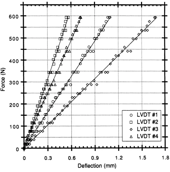
5.1 Load-deflection data for specimen A-1 loaded off-center by the URPP with all four edges clamped ... 105

5.2 Load-deflection data for specimen A-1 loaded off-center by the URPP with x edges simply supported and y edges clamped ... 106

5.3 Load-deflection data for specimen A-1 loaded off-center by the URPP with all four edges simply supported... 107

(14)

List of Figures (con't)

5.4 Load-deflection data for specimen A-1 loaded off-center by the

URPP with x edges free and y edges clamped ... 108 5.5 Load-deflection data for specimen A-1 loaded off-center by the

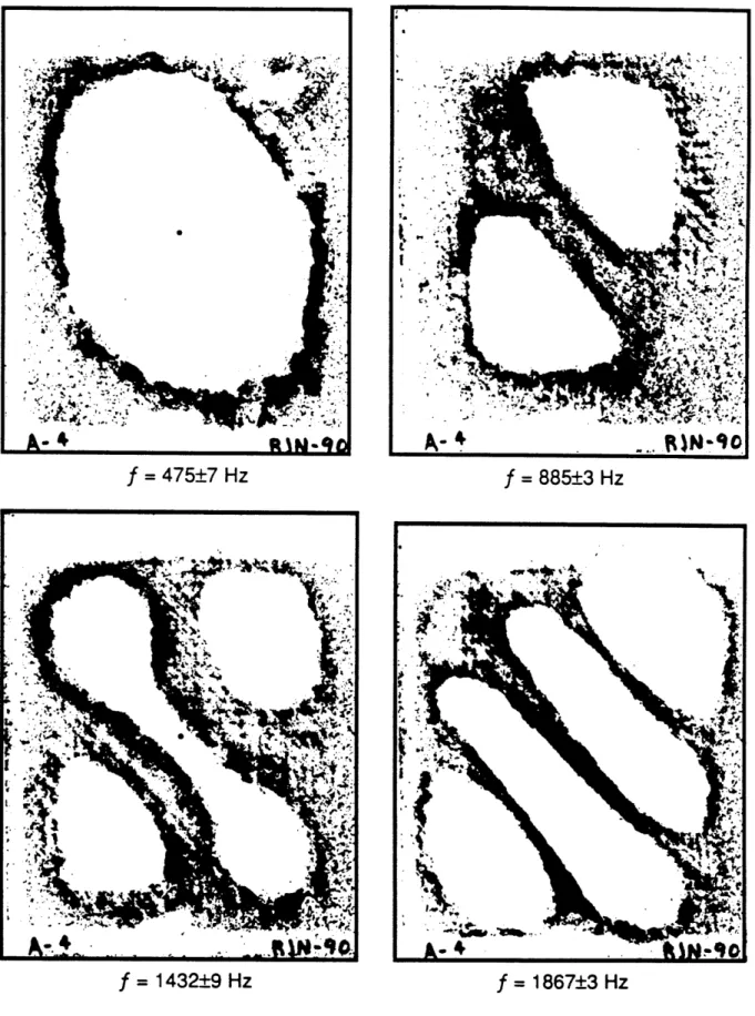
URPP with x edges free and y edges simply supported ... 109 5.6 Four lowest experimentally detected mode shapes and frequencies

for Specimen A with all four edges clamped ... 112 5.7 Four lowest experimentally detected mode shapes and frequencies

for Specimen B with all four edges clamped... ...113 5.8 Four lowest experimentally detected mode shapes and frequencies

for Specimen C with all four edges clamped...114 5.9 Four lowest experimentally detected mode shapes and frequencies

for Specimen D with all four edges clamped...115 5.10 Four lowest experimentally detected mode shapes and frequencies

for Specimen A with x edges (short edges) simply supported and y

edges (long edges) clamped... ...116 5.11 Four lowest experimentally detected mode shapes and frequencies

for Specimen B with x edges (short edges) simply supported and y

edges (long edges) clamped ... ...117 5.12 Four lowest experimentally detected mode shapes and frequencies

for Specimen C with x edges (short edges) simply supported and y

edges (long edges) clamped...118 5.13 Four lowest experimentally detected mode shapes and frequencies

for Specimen D with x edges (short edges) simply supported and y

edges (long edges) clamped...119 5.14 Four lowest experimentally detected mode shapes and frequencies

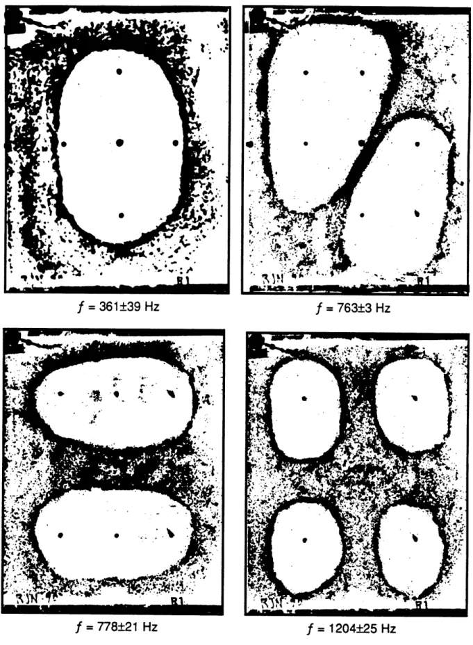
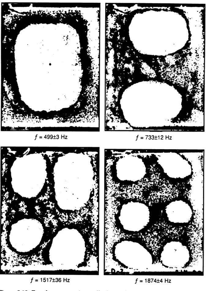
for Specimen A with all four edges simply supported ... 120 5.15 Four lowest experimentally detected mode shapes and frequencies

for Specimen B with all four edges simply supported ... 121 5.16 Four lowest experimentally detected mode shapes and frequencies

for Specimen C with all four edges simply supported ... 122 5.17 Four lowest experimentally detected mode shapes and frequencies

(15)

Fiure

_PEage

5.18 Four lowest experimentally detected mode shapes and frequencies for Specimen A with x edges (short edges) free and y edges (long

edges) clamped ... . ... 124 5.19 Four lowest experimentally detected mode shapes and frequencies

for Specimen B with x edges (short edges) free and y edges (long

edges) clam ped ... 125 5.20 Four lowest experimentally detected mode shapes and frequencies

for Specimen C with x edges (short edges) free and y edges (long

edges) clamped ... ... 126 5.21 Four lowest experimentally detected mode shapes and frequencies

for Specimen D with x edges (short edges) free and y edges (long

edges) clam ped ... 127 5.22 Four lowest experimentally detected mode shapes and frequencies

for Specimen A with x edges (short edges) free and y edges (long

edges) sim ply supported...128 5.23 Four lowest experimentally detected mode shapes and frequencies

for Specimen B with x edges (short edges) free and y edges (long

edges) simply supported ... 129 5.24 Four lowest experimentally detected mode shapes and frequencies

for Specimen C with x edges (short edges) free and y edges (long

edges) simply supported ... 130 5.25 Four lowest experimentally detected mode shapes and frequencies

for Specimen D with x edges (short edges) free and y edges (long

edges) simply supported ... 131 6.1 Comparison of Kirchhoff and Mindlin deformations for Specimen

B under a centered point load of 100 Newtons with all four edges

clamped ... 134 6.2 Convergence trend of Rayleigh-Ritz solution for Specimen B with

four edges clamped and a centered point load... 137 6.3 Convergence trend of constrained Navier solution for Specimen B

with four edges clamped and a centered point load ... 138 6.4 Transverse deflection for Specimen A, under a centered point load

of 100 Newtons, with all four sides clamped... 141 6.5 Transverse deflection for Specimen B, under a centered point load

(16)

6.6 Transverse deflection for Specimen C, under a centered point load

of 100 Newtons, with all four sides clamped ... 143 6.7 Transverse deflection for Specimen D, under a centered point load

of 100 Newtons, with all four sides clamped...144 6.8 Transverse deflection for Specimen I, under a centered point load

of 100 Newtons, with all four sides clamped ... 145 6.9 Transverse deflection for Specimen A, under a centered point load

of 100 Newtons, with all four sides simply supported...146 6.10 Transverse deflection for Specimen B, under a centered point load

of 100 Newtons, with all four sides simply supported...147 6.11 Transverse deflection for Specimen C, under a centered point load

of 100 Newtons, with all four sides simply supported ... 148 6.12 Transverse deflection for Specimen D, under a centered point load

of 100 Newtons, with all four sides simply supported...149 6.13 Transverse deflection for Specimen I, under a centered point load

of 100 Newtons, with all four sides simply supported...150 6.14 Transverse deflection for Specimen A, under an off-center point

load of 100 Newtons, with all four sides clamped ... 152 6.15 Transverse deflection for Specimen B, under an off-center point

load of 100 Newtons, with all four sides clamped ... 153 6.16 Transverse deflection for Specimen C, under an off-center point

load of 100 Newtons, with all four sides clamped ... 54 6.17 Transverse deflection for Specimen D, under an off-center point

load of 100 Newtons, with all four sides clamped ... 155 6.18 Transverse deflection for Specimen I, under an off-center point

load of 100 Newtons, with all four sides clamped ... ...156 6.19 Transverse deflection for Specimen A, under an off-center point

load of 100 Newtons, with x edges (short edges) simply supported

and y edges (long edges) clamped ... ...157 6.20 Transverse deflection for Specimen B, under an off-center point

(17)

6.21 Transverse deflection for Specimen C, under an off-center point load of 100 Newtons, with x edges (short edges) simply supported

and y edges (long edges) clamped... 159 6.22 Transverse deflection for Specimen D, under an off-center point

load of 100 Newtons, with x edges (short edges) simply supported

and y edges (long edges) clamped... 160 6.23 Transverse deflection for Specimen I, under an off-center point

and y edges (long edges) clamped ... 161 6.24 Transverse deflection for Specimen A, under an off-center point

load of 100 Newtons, with all four sides simply supported ... ... 162 6.25 Transverse deflection for Specimen B, under an off-center point

load of 100 Newtons, with all four sides simply supported ... 163 6.26 Transverse deflection for Specimen C, under an off-center point

load of 100 Newtons, with all four sides simply supported ... 164 6.27 Transverse deflection for Specimen D, under an off-center point

load of 100 Newtons, with all four sides simply supported ... 165 6.28 Transverse deflection for Specimen I, under an off-center point

load of 100 Newtons, with all four sides simply supported ... 166 6.29 Transverse deflection for Specimen A, under a centered URPP

load of 100 Newtons, with all four sides clamped ... 168 6.30 Transverse deflection for Specimen B, under a centered URPP

load of 100 Newtons, with all four sides clamped... 169 6.31 _{Transverse deflection for Specimen C, under a centered URPP}

load of 100 Newtons, with all four sides clamped... 170 6.32 Transverse deflection for Specimen D, under a centered URPP

load of 100 Newtons, with all four sides clamped ... ... 171 6.33 Transverse deflection for Specimen I, under a centered URPP

load of 100 Newtons, with all four sides clamped... 172 6.34 Transverse deflection for Specimen A, under a centered URPP

load of 100 Newtons, with all four sides simply supported ... 173 6.35 Transverse deflection for Specimen B, under a centered URPP

(18)

6.36 Transverse deflection for Specimen C, under a centered URPP

load of 100 Newtons, with all four sides simply supported ... 175 6.37 Transverse deflection for Specimen D, under a centered URPP

load of 100 Newtons, with all four sides simply supported...176 6.38 Transverse deflection for Specimen I, under a centered URPP

load of 100 Newtons, with all four sides simply supported... ...177 6.39 Transverse deflection for Specimen A, under an off-center URPP

load of 100 Newtons, with all four sides clamped ... 179 6.40 Transverse deflection for Specimen B, under an off-center URPP

load of 100 Newtons, with all four sides clamped ... 180 6.41 Transverse deflection for Specimen C, under an off-center URPP

load of 100 Newtons, with all four sides clamped ... 181 6.42 Transverse deflection for Specimen D, under an off-center URPP

load of 100 Newtons, with all four sides clamped ... ...182 6.43 Transverse deflection for Specimen I, under an off-center URPP

load of 100 Newtons, with all four sides clamped ... 183 6.44 Transverse deflection for Specimen A, under an off-center URPP

and y edges (long edges) clamped ... ... 184 6.45 Transverse deflection for Specimen B, under an off-center URPP

and y edges (long edges) clamped ... 185 6.46 Transverse deflection for Specimen C, under an off-center URPP

and y edges (long edges) clamped ... 186 6.47 Transverse deflection for Specimen D, under an off-center URPP

and y edges (long edges) clamped ... 187 6.48 Transverse deflection for Specimen I, under an off-center URPP

and y edges (long edges) clamped ... 188 6.49 Transverse deflection for Specimen A, under an off-center URPP

(19)

6.50 Transverse deflection for Specimen B, under an off-center URPP

load of 100 Newtons, with all four sides simply supported ... 190 6.51 Transverse deflection for Specimen C, under an off-center URPP

load of 100 Newtons, with all four sides simply supported ... 191 6.52 Transverse deflection for Specimen D, under an off-center URPP

load of 100 Newtons, with all four sides simply supported ... 192 6.53 Transverse deflection for Specimen I, under an off-center URPP

load of 100 Newtons, with all four sides simply supported ... 193 6.54 Transverse deflection for Specimen A, under a uniform pressure

load of 100 Newtons, with all four sides clamped ... 195 6.55 Transverse deflection for Specimen B, under a uniform pressure

load of 100 Newtons, with all four sides clamped... 196 6.56 Transverse deflection for Specimen C, under a uniform pressure

load of 100 Newtons, with all four sides clamped ... 197 6.57 Transverse deflection for Specimen D, under a uniform pressure

load of 100 Newtons, with all four sides clamped ... 198 6.58 Transverse deflection for Specimen I, under a uniform pressure

load of 100 Newtons, with all four sides clamped... 199 6.59 Transverse deflection for Specimen A, under a uniform pressure

and y edges (long edges) clamped... 200 6.60 Transverse deflection for Specimen B, under a uniform pressure

and y edges (long edges) clamped... 201 6.61 Transverse deflection for Specimen C, under a uniform pressure

and y edges (long edges) clamped... 202 6.62 Transverse deflection for Specimen D, under a uniform pressure

and y edges (long edges) clamped ... 203 6.63 Transverse deflection for Specimen I, under a uniform pressure

(20)

6.64 Transverse deflection for Specimen A, under a uniform pressure

load of 100 Newtons, with all four sides simply supported... 205 6.65 Transverse deflection for Specimen B, under a uniform pressure

load of 100 Newtons, with all four sides simply supported... .. 206 6.66 Transverse deflection for Specimen C, under a uniform pressure

load of 100 Newtons, with all four sides simply supported ... ...207 6.67 Transverse deflection for Specimen D, under a uniform pressure

load of 100 Newtons, with all four sides simply supported...208 6.68 Transverse deflection for Specimen I, under a uniform pressure

load of 100 Newtons, with all four sides simply supported... ...209 6.69 First four natural mode shapes and frequencies for Specimen A

with all four edges clamped ... 211 6.70 First four natural mode shapes and frequencies for Specimen B

with all four edges clamped ... ... 212 6.71 First four natural mode shapes and frequencies for Specimen C

with all four edges clamped ... 213 6.72 First four natural mode shapes and frequencies for Specimen D

with all four edges clamped ...214 6.73 First four natural mode shapes and frequencies for Specimen I

with all four edges clamped ... 215 6.74 First four natural mode shapes and frequencies for Specimen A

with x edges (short edges) simply supported and y edges (long

edges) clamped ... 216 6.75 First four natural mode shapes and frequencies for Specimen B

edges) clam ped... 217 6.76 First four natural mode shapes and frequencies for Specimen C

edges) clam ped... 218 6.77 First four natural mode shapes and frequencies for Specimen D

(21)

Figure

"eer

6.78 First four natural mode shapes and frequencies for Specimen I with x edges (short edges) simply supported and y edges (long

edges) clam ped ... 220 6.79 First four natural mode shapes and frequencies for Specimen A

with all four edges simply supported ... 221 6.80 First four natural mode shapes and frequencies for Specimen B

with all four edges simply supported ... 222 6.81 First four natural mode shapes and frequencies for Specimen C

with all four edges simply supported ... 223 6.82 First four natural mode shapes and frequencies for Specimen D

with all four edges simply supported ... 224 6.83 First four natural mode shapes and frequencies for Specimen I

with all four edges simply supported ... 225 7.1 Transverse deflection for Specimen A, under a centered point load

of 100 Newtons, with all four sides clamped... 231 7.2 Transverse deflection for Specimen B, under a centered point load

of 100 Newtons, with all four sides clamped... 232 7.3 Transverse deflection for Specimen C, under a centered point load

of 100 Newtons, with all four sides clamped... 233 7.4 Transverse deflection for Specimen D, under a centered point load

of 100 Newtons, with all four sides clamped... 234 7.5 Transverse deflection for Specimen I, under a centered point load

of 100 Newtons, with all four sides clamped... 235 7.6 Transverse deflection for Specimen A, under a centered point load

of 100 Newtons, with all four sides simply supported ... 236 7.7 Transverse deflection for Specimen B, under a centered point load

of 100 Newtons, with all four sides simply supported ... 237 7.8 Transverse deflection for Specimen C, under a centered point load

of 100 Newtons, with all four sides simply supported ... 238 7.9 Transverse deflection for Specimen D, under a centered point load

of 100 Newtons, with all four sides simply supported ... 239 7.10 Transverse deflection for Specimen I, under a centered point load

(22)

7.11 Transverse deflection for Specimen A, under an off-center point

load of 100 Newtons, with all four sides clamped ... 242 7.12 Transverse deflection for Specimen B, under an off-center point

load of 100 Newtons, with all four sides clamped ... ...243 7.13 Transverse deflection for Specimen C, under an off-center point

load of 100 Newtons, with all four sides clamped ... 244 7.14 Transverse deflection for Specimen D, under an off-center point

load of 100 Newtons, with all four sides clamped ... 245 7.15 Transverse deflection for Specimen I, under an off-center point

load of 100 Newtons, with all four sides clamped ... 246 7.16 Transverse deflection for Specimen A, under an off-center point

and y edges (long edges) clamped ... ... 247 7.17 Transverse deflection for Specimen B, under an off-center point

and y edges (long edges) clamped ... 248 7.18 Transverse deflection for Specimen C, under an off-center point

and y edges (long edges) clamped ... 249 7.19 Transverse deflection for Specimen D, under an off-center point

and y edges (long edges) clamped ... 250 7.20 Transverse deflection for Specimen I, under an off-center point

and y edges (long edges) clamped ... 251 7.21 Transverse deflection for Specimen A, under an off-center point

load of 100 Newtons, with all four sides simply supported ... 252 7.22 Transverse deflection for Specimen B, under an off-center point

load of 100 Newtons, with all four sides simply supported ... 253 7.23 Transverse deflection for Specimen C, under an off-center point

load of 100 Newtons, with all four sides simply supported...254 7.24 Transverse deflection for Specimen D, under an off-center point

(23)

7.25 Transverse deflection for Specimen I, under an off-center point

load of 100 Newtons, with all four sides simply supported ... 256 7.26 Transverse deflection for Specimen A, under a centered URPP

load of 100 Newtons, with all four sides clamped ... 258 7.27 Transverse deflection for Specimen B, under a centered URPP

load of 100 Newtons, with all four sides clamped... 259 7.28 Transverse deflection for Specimen C, under a centered URPP

load of 100 Newtons, with all four sides clamped ... 260 7.29 Transverse deflection for Specimen D, under a centered URPP

load of 100 Newtons, with all four sides clamped... 261 7.30 Transverse deflection for Specimen I, under a centered URPP

load of 100 Newtons, with all four sides clamped...62 7.31 Transverse deflection for Specimen A, under a centered URPP

load of 100 Newtons, with all four sides simply supported ... 263 7.32 Transverse deflection for Specimen B, under a centered URPP

load of 100 Newtons, with all four sides simply supported ... 264 7.33 Transverse deflection for Specimen C, under a centered URPP

load of 100 Newtons, with all four sides simply supported ... 265 7.34 Transverse deflection for Specimen D, under a centered URPP

load of 100 Newtons, with all four sides simply supported ... 266 7.35 Transverse deflection for Specimen I, under a centered URPP

load of 100 Newtons, with all four sides simply supported ... 267 7.36 Transverse deflection for Specimen A, under an off-center URPP

load of 100 Newtons, with all four sides clamped ... 269 7.37 Transverse deflection for Specimen B, under an off-center URPP

load of 100 Newtons, with all four sides clamped... 270 7.38 Transverse deflection for Specimen C, under an off-center URPP

load of 100 Newtons, with all four sides clamped... . 271 7.39 Transverse deflection for Specimen D, under an off-center URPP

load of 100 Newtons, with all four sides clamped... 272 7.40 Transverse deflection for Specimen I, under an off-center URPP

(24)

Figure

Page

7.41 Transverse deflection for Specimen A, under an off-center URPP load of 100 Newtons, with x edges (short edges) simply supported

and y edges (long edges) clamped ... 274 7.42 Transverse deflection for Specimen B, under an off-center URPP

and y edges (long edges) clamped ... 275 7.43 Transverse deflection for Specimen C, under an off-center URPP

and y edges (long edges) clamped ... 276 7.44 Transverse deflection for Specimen D, under an off-center URPP

and y edges (long edges) clamped ... 277 7.45 Transverse deflection for Specimen I, under an off-center URPP

and y edges (long edges) clamped ... 278 7.46 Transverse deflection for Specimen A, under an off-center URPP

load of 100 Newtons, with all four sides simply supported...279 7.47 Transverse deflection for Specimen B, under an off-center URPP

load of 100 Newtons, with all four sides simply supported...280 7.48 Transverse deflection for Specimen C, under an off-center URPP

load of 100 Newtons, with all four sides simply supported...281 7.49 Transverse deflection for Specimen D, under an off-center URPP

load of 100 Newtons, with all four sides simply supported...282 7.50 Transverse deflection for Specimen I, under an off-center URPP

load of 100 Newtons, with all four sides simply supported...283 7.51 Transverse deflection for Specimen A, under a uniform pressure

load of 100 Newtons, with all four sides clamped ... 285 7.52 Transverse deflection for Specimen B, under a uniform pressure

load of 100 Newtons, with all four sides clamped ... 286 7.53 Transverse deflection for Specimen C, under a uniform pressure

load of 100 Newtons, with all four sides clamped ... 287 7.54 Transverse deflection for Specimen D, under a uniform pressure

(25)

Figure

Page

7.55 Transverse deflection for Specimen I, under a uniform pressure

load of 100 Newtons, with all four sides clamped... 289 7.56 Transverse deflection for Specimen A, under a uniform pressure

and y edges (long edges) clamped... 290 7.57 Transverse deflection for Specimen B, under a uniform pressure

and y edges (long edges) clamped... 291 7.58 Transverse deflection for Specimen C, under a uniform pressure

and y edges (long edges) clamped... 292 7.59 Transverse deflection for Specimen D, under a uniform pressure

and y edges (long edges) clamped... 293 7.60 Transverse deflection for Specimen I, under a uniform pressure

and y edges (long edges) clamped ... ... 294 7.61 Transverse deflection for Specimen A, under a uniform pressure

load of 100 Newtons, with all four sides simply supported ... 295 7.62 Transverse deflection for Specimen B, under a uniform pressure

load of 100 Newtons, with all four sides simply supported ... 296 7.63 Transverse deflection for Specimen C, under a uniform pressure

load of 100 Newtons, with all four sides simply supported ... ... 297 7.64 Transverse deflection for Specimen D, under a uniform pressure

load of 100 Newtons, with all four sides simply supported ... 298 7.65 Transverse deflection for Specimen I, under a uniform pressure

load of 100 Newtons, with all four sides simply supported... 299 7.66 Comparison of first and second experimental and analytical

modes for Specimen B with all four edges simply supported... 302 7.67 Comparison of third and fourth experimental and matching

analytical modes for Specimen B with all four edges simply

(26)

(27)

List of Tables

Table Pa•

2.1 Dugundji Beam Mode Shape Parameters...55 3.1 Extra Plate Length per Edge Required for Boundary Conditions ... 60 3.2 Laminate Designations and Inherent Couplings ... 66 3.3 Test Specimen Average Thicknesses...72 3.4 Test M atrix ... ... 86 4.1 Nominal Cured Ply Properties...87 4.2 In-plane Laminate Stiffnesses... 88 4.3 Transverse Laminate Stiffnesses ... 89 5.1 Experimental Modal Frequencies (Hz) for Aluminum Control

Plates ... ... 111 6.1 Comparison of Natural Frequencies (Hz) for Specimen B with

Four Edges Simply Supported ... 135 6.2 Comparison of Natural Frequencies (Hz) for Specimen I with

Four Edges Simply Supported... 136 7.1 Difference of Experimental Stiffness from Rayleigh-Ritz

Prediction ... ... 229 7.2 Difference of Experimental Frequency from Rayleigh-Ritz

Prediction ... 300 A.1 Thickness Measurements for A and B Specimens (mm)... 314 A.2 Thickness Measurements for C and D Specimens (mm)... 315 G. 1 Experimental Stiffnesses for Centered Point Load (CL-CL)...354 G.2 Experimental Stiffnesses for Centered Point Load (SS-SS)... 355 G.3 Experimental Stiffnesses for Off-Center Point Load (CL-CL)... 356 G.4 Experimental Stiffnesses for Off-Center Point Load (SS-CL) ...357 G.5 Experimental Stiffnesses for Off-Center Point Load (SS-SS) ... 358 G.6 Experimental Stiffnesses for Off-Center Point Load (FR-CL)... 359 G.7 Experimental Stiffnesses for Off-Center Point Load (FR-SS) ...360

(28)

List of Tables (con't)

Table

Page

G.8 Experimental Stiffnesses for Centered URPP (CL-CL)... 361 G.9 Experimental Stiffnesses for Centered URPP (SS-SS) ... 362 G.10 Experimental Stiffnesses for Off-Center URPP (CL-CL)... 363 G.11 Experimental Stiffnesses for Off-Center URPP (SS-CL) ... ..364 G.12 Experimental Stiffnesses for Off-Center URPP (SS-SS) ... 365 G.13 Experimental Stiffnesses for Off-Center URPP (FR-CL) ... 366 G.14 Experimental Stiffnesses for Off-Center URPP (FR-SS) ... 367 G. 15 Experimental Stiffnesses for Uniform Pressure (CL-CL) ... 368 G.16 Experimental Stiffnesses for Uniform Pressure (SS-CL)...369 G.17 Experimental Stiffnesses for Uniform Pressure (SS-SS) ... 370 H.1 Navier Stiffnesses for Centered Point Load Cases ... ...372 H.2 Navier Stiffnesses for Off-Center Point Load Cases ... 372 H.3 Navier Stiffnesses for Centered URPP Cases...373

H.4 Navier Stiffnesses for Off-Center URPP Cases ... 373 H.5 Navier Stiffnesses for Uniform Pressure Cases ... 374 H.6 Rayleigh-Ritz Stiffnesses for Centered Point Load Cases .... ... 375 H.7 Rayleigh-Ritz Stiffnesses for Off-Center Point Load Cases ... ....375 H.8 Rayleigh-Ritz Stiffnesses for Centered URPP Cases...376 H.9 Rayleigh-Ritz Stiffnesses for Off-Center URPP Cases...376 H.10 Rayleigh-Ritz Stiffnesses for Uniform Pressure Cases... ...377 H.11 Potential Function Stiffnesses for Centered Point Load Cases ... 378 H.12 Potential Function Stiffnesses for Centered URPP Cases ... 378 H.13 Potential Function Stiffnesses for Uniform Pressure Cases ... ... 379

(29)

Nomenclature

A1 Amplitude of potential function

Aq Plate extensional stiffness matrix a Plate dimension in x direction Bij Plate coupling stiffness matrix b Plate dimension in y direction Cii Transverse shear stiffnesses Dij Plate bending stiffness matrix

fx, fy, fz Body forces in the x, y, and z directions

h Plate thickness

iij Constants which arise from the differential operators Lij Differential operators

mx, my Surface tractions in the x and y directions

Mx, My, Mxy Moment resultants

Nx, Ny, Nxy Stress resultants

Px, Py Body force resultants

Pz Distributed transverse loading qj Reduced in-plane stiffnesses

Ox, Qy Transverse shear stress resultants Ro, R1, R2 Integrated inertia terms

u Plate displacement in x direction uO Midplane displacement in x direction v Plate displacement in y direction vo Midplane displacement in y direction w Midplane displacement in z direction x, y, z Plate coordinates

(30)

y Engineering shear strain

e Extensional strain

iK Shear correction factor

p density

a Extensional stress

t Shear stress

QD Potential function

Tx Shear rotation of the undeformed normal w.r.t the y-z plane

(31)

Chapter 1 Introduction

Composite materials pose rewarding challenges to the structural engineer familiar with isotropic materials. Strength becomes a function of direction in the material, failure occurs in many diverse and sometimes unrelated modes, and bending behavior can be materially coupled with in-plane behavior. Although still the exception rather the the norm, composites are finding their way into an ever increasing number of applications, from high tech sports equipment to primary aircraft structure, where their high strength to weight ratio makes them attractive alternatives to their isotropic predecessors. As the use of composites increases, more and more engineers will discard their anisophobia and open their minds to the wonders of an anisotropic world.

A single ply, or layer, of composite material is orthotropic. By rotating individual plies through different angles and laminating them together, however, complicated material couplings can be created. These material couplings, which arise due to the laminate's anisotropic nature, can significantly affect the laminate's mechanical properties. Engineers should carefully include the effects of these couplings when necessary, in order to fully utilize composites, rather than avoiding all couplings due to a lack of understanding.

This work investigates the effects of twisting and bending-shearing coupling in laminates subjected to three static, transverse loadings and a dynamic transverse vibration. The experimental results are compared with analytical solutions to determine the quality of the modeling and the effect of the couplings for the loadings and boundary conditions considered.

(32)

Additionally, a new displacement based potential function solution is presented.

Chapter two provides a general background from the literature on the subject of anisotropic plate bending. Both Kirchhoff and Mindlin plate theories are considered, and typical solution techniques are discussed. The experimental procedures for specimen manufacture and testing are detailed in chapter three. Chapter four describes the analyses used, and explains the displacement based potential function solution.

The extensive experimental results are presented in chapter five, followed by the analytical results in chapter six. Comparisons of the experimental and analytical results are then made in chapter seven. Finally, chapter eight provides a concise summary of the conclusions of this investigation and suggestions for future work.

(33)

Chapter 2

Summary of Previous Work

This chapter briefly summarizes previous composite plate analysis techniques. The solution of a plate problem consists of an underlying theory, or model of the plate, and a solution technique, or mathematical procedure, for approximating the response of a plate to a given loading, for a particular set of boundary conditions. In general, a solution technique may be applied to several different theories, and a theory may be solved using any of several solution techniques. The relation is not always this clear cut, however, as some theories lend themselves more readily to some solution techniques than others.

2.1 Plate Theories

Thousands of papers have been written on the topics of plate theories and solutions to plate theories; even hundreds of papers have been written concerning laminated orthotropic and anisotropic plates. Many of these plate theories and solution techniques are highly specialized and are applicable or useful for only a small class of problems. Only those theories which are general enough to be applied to a broad class of engineering problems are discussed here.

2.1.1 Kirchhoff Plate Theory

The "classical" plate theory or Kirchhoff plate theory [1] uses three midplane displacement variables. The in-plane displacements, uo and vo, are the midplane displacements in the x and y directions respectively. The out-of-plane displacement, w, is the displacement in the z direction, or the

(34)

displacement normal to the plane of the plate. The displacement field is as follows:

aw aw

u = uo(x,y,t) - z - v = vo(x,y,t) - z -- , w = w(x,y,t)

ax

ay

Kirchhoff plate theory assumes that as a plate deforms an imaginary plane originally normal to the midplane will remain planer and normal to the midplane throughout the deformation, see Figure 2.1. This implies that the transverse shear strains will be approximately zero. The negligible transverse shear strain assumption is acceptable for "thin" plates with "moderate" transverse shear stiffness, but becomes less accurate with increasing plate thickness or decreasing transverse shear stiffness. A plate is classified as "thin" if the shorter edge length to thickness ratio is greater than one hundred. Generally, transverse shear stiffness is considered "moderate" if the ratio of in-plane stiffness to transverse shear stiffness is around 2.5.

Kirchhoff plate theory is an integrated plate theory. Quantities are integrated through the thickness, which simplifies the model, but usually results in pointwise breaches of equilibrium. The integrated loadings, or resultants, are defined as:

Nxj= c xdz; Ny= aydz; Nxy = xy dz

2 2 2

1 h h

Mx = jx z dz; My = jya zdz; Mxy = fTxy zdz

2 2 2

2 2_

Qx= x••z dz; Qy= tyz dz

(35)

aw '-7 oax

ne

deformed plate

I

IP

midplane

undeformed plate

Figure 2.1 Kirchhoff plate theory deformation. Plane sections remain plane and normal to the midplane throughout deformation.

(36)

Px = fx dz ; Py = fy dz;

2

h

Pz = fz dz + Pz

2

where the Ni's are stress resultants, the Mi's are moment resultants, the Qi's are transverse shear stress resultants, and px and py are body force resultants arising from the body forces, fx and fy. The distributed transverse load, Pz, is the sum of the applied transverse load, Pz, and the integrated loading due to a body force, fz. Additionally, the plate may rest on a frictionless, uniform elastic foundation with stiffness K. The Kirchhoff plate model is depicted in Figure 2.2.

The integrated stiffnesses are defined as:

Aij = Qij dz ; 2 Bij= Oij z dz ; 2 Dii= Qij Z2 _{dz ;} 2

where the Qij's are the ply, reduced in-plane stiffnesses [2]. The integrated inertia terms are defined as follows:

h Ro= p dz; 2 h

R, =

P

z

dz; 2 (i,j = 1,2,6)

h

R2 = p z2 dz 2

(37)

b

Nxo

l b

a

f

xx

/~

6

Mx

z

Fu

2f1777

Y

Nu.~

,P

\

cIc

1777

(38)

The constitutive equations follow as: N_x Ny Nxy Mx All _A₁₂ A₁₂ A₂₂ A₁₆ _A₂₆ B₁₁ _B₁₂ B₁₂ B₁₆ B₂₂ B₂₆

The strain-displacement relations, are:

cx

=

-u

x

;

Kx = - W, xx ;

in accordance with the displacement field,

'y = Uy + Vx Kxy = - 2, xy

where the comma designates differentiation with respect to the variables that follow.

From the constitutive equations and the strain-displacement relations, we see that the Bij terms, or coupling stiffnesses, couple the in-plane and

out-of-plane displacements. Finally, the equations of motion are [3]: L₁₂ L22 L23

L13 Uo

-px

L23 Vo = -Py L33 LW +Pz

where the Lij's are differential operators defined as: B11 B₁₂ B₁₆ A₁₆ A₂₆ A₆₆ B₁₆ B₂₆ B₆₆ B₁₂ _B₁₆ B₂₂ _B_{2 6} B₂₆ _B₆₆ D₁₂ _D₁₆ D₂₂ _D₂₆ D₂₆ D₆₆

0

Kx Sxy

y

= ?-

w,

y;

Ily = -W, yy;

(39)

L11 = All Lxx + 2 A16 Lxy + A66 Lyy - RO Ltt

L12 = A16 _{Lxx + (A12 + A}_{6 6}_{) Lxy +}_A_{2 6}_Lyy

L13 = -811 Lxxx - 3 B16 Lxxy-(B12 + 2 866) Lxyy- B26 Lyyy + R1 Lxtt

L22 = A66 Lxx + 2 A26 Lxy + A22 Lyy - Ro Ltt

L23 = -B16 Lxxx - (B12 + 2 B6 6) Lxxy - 3 B2 6 Lxyy - 22 Lyyy + R1 Lytt

L33 = D11 Lxxxx + 4 D1 6 Lxxxy + 2 (D12 + 2 D_{6 6}) Lxxyy + 4 D_{2 6}Lxyyy + D₂₂Lyyyy

+ K + R0 Ltt - R2 Lxxtt - R2 Lyytt

where:

a

2

_a

3

_a

4

Lxx = ; Lxxy = ; Lxxtt =

aXWx2ay 2 ax2at2

and the other partial derivatives are defined similarly.

The equations of motion may be solved with sufficient initial and boundary conditions. For example, along an x edge any combination of the following boundary conditions may be prescribed:

UO or Nx

vo or Nxy

w or Qx+Mxy, y

W,x or Mx

These governing partial differential equations and boundary conditions summarize the Kirchhoff plate theory. For thin plates with moderate transverse shear stiffness these equations are a reasonable model, however, in other cases transverse shear deformation should be accounted for.

2.1.2 Mindlin Plate Theory

For thick plates or plates with a low transverse shear stiffness, rotations of the midplane normals must be included for accurate modeling. Shear

(40)

deformation plate theory or Mindlin plate theory [4] uses five displacement variables. The midplane displacements are uo and vo as before, however, two out-of-plane shear rotations, Tx and Py, are introduced. The out-of-plane displacement, w, remains defined as in Kirchhoff plate theory. The new displacement field is as follows:

u = uo(x,y,t) + z Yx(x,y,t); v = vo(x,y,t) + z 'y(x,y,t); w = w(x,y,t)

Mindlin plate theory assumes that as a plate deforms an imaginary plane originally normal to the midplane will remain planer, but will rotate from the midplane normal during deformation, see Figure 2.3. This allows non-zero transverse shear strains. Mindlin plate theory more accurately models thick plates or plates with low transverse shear stiffness.

Mindlin plate theory is also an integrated plate theory. The integrated loadings, body force resultants, and distributed transverse load are all defined as they were in Kirchhoff plate theory. Distributed surface tractions, mx and my, may also be applied to the upper surface of the plate [5, 61. Recall that the uniform elastic foundation is assumed frictionless, thus not causing surface tractions on the lower side of the plate. The Mindlin plate model is depicted in Figure 2.4.

The integrated in-plane stiffnesses are defined as in Kirchhoff plate theory, however, additional transverse shear stiffnesses are needed. Traditionally, the transverse shear stiffnesses have been defined as [3]:

(41)

'Ix ow \ Dxz XZ I

ax

'Yxz "11 \_I _I \

midplane

deformed plate

midplane

undeformed plate

Figure 2.3 Mindlin plate theory deformation. Plane sections remain plane but rotate from the midplane normal throughout deformation.

(42)

my

Mindlin plate model with applied loadings.

(43)

where the Cij's are the ply transverse shear stiffnesses [2]. Recently, several authors [7, 8] have proposed a different formulation of the transverse stiffnesses for laminated plates. The alternative formulation is based on 3-D elasticity and allows a weighted average, very similar to springs in series, of the individual transverse shear stiffnesses. The alternative transverse shear stiffnesses are defined as follows:

A

44

A

45

h S44

S45

A45 A55 S45 S55 h

Sij = - Sij dz

where the Sij's are the ply compliances [2], and h is the plate thickness. For a plate laminated from layers of the same material the difference in transverse shear stiffness between the two methods is small. If, however, the plate is laminated from materials with significantly different ply transverse shear stiffnesses, the resulting laminate transverse stiffnesses will be very different.

Having defined all the plate stiffnesses, the constitutive equations may be expressed as follows [9]:

(44)

N_x Ny Nxy Mx My Mxy

Oy

A44

A45

yz

Ox A₄₅ A55 Yxz

The transverse shear stiffnesses have been multiplied by a shear correction factor, K, following Mindlin [4] and others [3,5,91. This is to account for the inaccuracies inherent in assuming the shear stress is constant through the thickness, while the boundary conditions guarantee the shear stress goes to zero at the plate surfaces. Care should be taken to differentiate between the shear correction factor which has no subscripts and the curvatures which have subscripts. The strain-displacement relations are found from the displacement field. The in-plane strains remain as defined for Kirchhoff plate theory, however, the curvatures and transverse shear strains are now defined as follows:

Kx = 'x,x ; Ky = y, ; Kx y = Yx, y + Py, x Yyz = W,y + 'y; Yxz = W,x + 'x

Finally, the equations of motion are as follows [5]:

All A12 A1 6 B11 B12 B1 6 A₁₂ A22 A26 B12 B22 B2 6 A₁₆ A_{2 6} A₆₆ B16 B26 B6 6 B₁₁ B1 2 B16 D11 D1 2 D1 6 B1 2 B2 2 B2 6 D12 D2 2 D2 6 B16 B2 6 B6 6 D16 D2 6 D6 6 Ox Kx Kx y

KX y

(45)

Ll, L₁₂ L13 L14 L15 L1 2 L22 L23 L24 L25 L13 L23 L3 3 L34 L3 5 L1 4 L24 L34 L44 L45 L15 L25 L35 L4 5 L55 UO VO

W

wX IvY -Px -PY -Pz +mx +my

where the Lij's are differential operators defined as:

Ll1 = All Lxx + 2 A16 Lxy + A66 Lyy - R Ltt

L12 = A16 Lxx + (A12 + A66) Lxy + A26 Lyy

L13 = 0

L14 = B1 1 Lxx + 2 B16 Lxy + B66 Lyy - R Ltt

L15 = B16 Lxx + (B12 + B66) Lxy + B26 Lyy

L22 = A6 6 Lxx + 2 A26 Lxy + A22 Lyy - RO Ltt

L23 _{= 0}

L24 = B16 Lxx +(B12 + B66) Lxy + B26 Lyy

L2 5 = B66 Lxx + 2 B2 6 Lxy + B22 Lyy - R Ltt

L33 = K A55 Lxx + 2 K A45 Lxy + K A44 Lyy - K - RO Ltt

L34 = K A55 _{Lx + KA45 Ly}

L35 = K A45 Lx + xc A44 Ly

L4 4 = x A5 5 - Dl Lxx - 2 D16 Lxy - D6 6 Lyy + R2 Ltt

L_{4 5} = K A45 - D16 Lxx -(D1 2 + D66) Lxy - D26 Lyy

L55 = K A44 - D66 Lxx - 2 D26 Lxy- D22 Lyy + R2 Ltt

Again the equations of motion may be solved with sufficient initial and boundary conditions. Instead of four boundary conditions per edge, however, there are now five. For example, along an x edge any combination of the following boundary conditions may be prescribed:

(46)

uo or Nx

vO or Nxy

w or Qx

Tx or Mx

Sy _{or Mxy}

These governing partial differential equations and boundary conditions summarize the Mindlin plate theory. The Mindlin plate theory is useful in characterizing thick plates or plates with low transverse shear stiffness.

J. N. Reddy [10] has formulated a higher order shear deformation theory based on the same five displacement variables as Mindlin plate theory, but with a higher order displacement field for u and v. This theory is aesthetically pleasing because it allows the transverse shear stress distribution to be parabolic through the thickness, however, it effectively doubles the complexity of the plate bending problem. While Reddy's theory represents an improvement over Mindlin plate theory, this improvement is most significant for plates with a length to thickness ratio less than ten. For plates with a length to thickness ratio greater than ten, i.e. most engineering problems, the improvement is negligible and for that reason Reddy's theory will not be

discussed further here.

2.1.3 Symmetric Operator Reduction Method

V. Z. Vlasov observed that a series of partial differential equations describing the equilibrium of elastic solids will always have a symmetric matrix of differential operators. The symmetry is in accordance with Betti's reciprocal theorem and is insured as long as any elimination of higher order terms is done consistently [11].

(47)

Simply put, Betti's reciprocal theorem states that the flexibility influence coefficients for a linearly elastic solid will be symmetric [12]. If a unit generalized force at point 1 causes a generalized displacement at point 2 of wo, then a unit generalized force at point 2 will cause a generalized displacement at point 1, also of wo. The symmetry of the flexibility influence coefficients is directly related to the symmetry of the differential operator matrix.

For a symmetric operator matrix with constant coefficients, Vlasov found that the system of partial differential equations may be reduced to a single partial differential equation in terms of a potential function, whose order of differentiation is identical to that of the original system. Vlasov derived the eighth order partial differential equation governing the deflection of isotropic shells neglecting transverse shear deformation.

Vlasov's work with isotropic shells was later extended to orthotropic shells by S. A. Ambartsumyan [13]. While the expressions become more cumbersome with the added material complexity, the reduction method remains unchanged. Again Ambartsumyan's reduction used a Kirchhoff type shell theory, neglecting transverse shear. While much of Ambartsumyan's work dealt with anisotropic shells, he never applied the reduction method to the fully anisotropic case. This was done by Graves [14] in his Ph.D. thesis.

The symmetric operator reduction method is neither a plate theory nor a solution technique. Given a set of partial differential equations resulting from any plate theory that obeys Betti's reciprocal theorem, the reduction method allows the system of equations to be recast as a single equation in terms of a potential function. It is hoped that such recasting will promote unique and useful solutions.

(48)

2.2 Solution Techniaues

Once the equilibrium equations have been found for a particular plate theory, it remains to find a solution for specific boundary conditions and initial conditions. Applicability of solution techniques seems to be more dependent upon the particular boundary conditions of a problem than on the underlying plate theory used to formulate the problem.

2.2.1 Navier Solutions

Navier solutions expand the displacement functions as double Fourier sine and/or cosine series which are selected to explicitly satisfy all the boundary conditions. The solution utilizes the orthogonality of Fourier series by finding the Fourier expansion of the applied loading and then solving for the unknown coefficients through harmonic balance. Completeness of the solution is assured due to the completeness of the Fourier series themselves. Navier solutions are very numerically efficient but are applicable to a limited number of problems.

Navier solutions are possible for plates with all four sides simply supported, but are restricted to plates with no bending-stretching and no bending-twisting coupling. Without bending-stretching coupling the in-plane and out-of-plane problems are uncoupled. For a Kirchhoff plate bending problem this leaves one partial differential equation to be solved subject to two boundary conditions per edge; for a Mindlin plate bending problem this leaves a system of three partial differential equations to be solved subject to three boundary conditions per edge.

For a rectangular Kirchhoff plate of dimensions a by b, simply supported at x = 0, a and y = 0, b, the Navier solution assumes the transverse