Recolonisation by diffusion can generate increasing rates of spread

HAL Id: hal-00487738

https://hal.archives-ouvertes.fr/hal-00487738

HAL is a multi-disciplinary open access archive for the deposit and dissemination of sci-entific research documents, whether they are pub-lished or not. The documents may come from teaching and research institutions in France or

L’archive ouverte pluridisciplinaire HAL, est destinée au dépôt et à la diffusion de documents scientifiques de niveau recherche, publiés ou non, émanant des établissements d’enseignement et de recherche français ou étrangers, des laboratoires

Recolonisation by diffusion can generate increasing rates

of spread

Lionel Roques, François Hamel, Julien Fayard, Bruno Fady, Etienne Klein

To cite this version:

Lionel Roques, François Hamel, Julien Fayard, Bruno Fady, Etienne Klein. Recolonisation by diffusion can generate increasing rates of spread. Theoretical Population Biology, Elsevier, 2010, 77 (3), pp.205-212. �10.1016/j.tpb.2010.02.002�. �hal-00487738�

Recolonisation by diffusion can generate increasing rates of

spread

L. Roquesa,*, F. Hamelb , J. Fayarda , B. Fadyc and E.K. Kleina

a UR 546 Biostatistique et Processus Spatiaux, INRA, F-84000 Avignon, France b Aix-Marseille Universit´e, LATP, F-13397 Marseille, France & Institut Universitaire de France

and Helmholtz Zentrum M¨unchen, Institut f¨ur Biomathematik und Biometrie Ingolst¨adter Landstrasse 1, D-85764 Neuherberg, Germany

c UR 629 Ecologie des Forˆets M´editerran´eennes, INRA, F-84000 Avignon, France * Author for correspondence. (lionel.roques@avignon.inra.fr)

Abstract

Diffusion is one of the most frequently used assumptions to explain dispersal. Dif-fusion models and in particular reaction-difDif-fusion equations usually lead to solutions moving at constant speeds, too slow compared to observations. As early as 1899, Reid had found that the rate of spread of tree species migrating to northern envi-ronments at the beginning of the Holocene was too fast to be explained by diffusive dispersal. Rapid spreading is generally explained using long distance dispersal events, modelled through integro-differential equations (IDEs) with exponentially unbounded (EU) kernels, i.e. decaying slower than any exponential. We show here that classical reaction-diffusion models of the Fisher-Kolmogorov-Petrovsky-Piskunov type can pro-duce patterns of colonisation very similar to those of IDEs, if the initial population is EU at the beginning of the considered colonisation event. Many similarities between reaction-diffusion models with EU initial data and IDEs with EU kernels are found; in particular comparable accelerating rates of spread and flattening of the solutions. There was previously no systematic mathematical theory for such reaction-diffusion models with EU initial data. Yet, EU initial data can easily be understood as conse-quences of colonisation-retraction events and lead to fast spreading and accelerating rates of spread without the long distance hypothesis.

Keywords: reaction-diffusion; long distance; integro-differential; refugia; Reid’s para-dox

1

Introduction

Since the work of Skellam (1951), reaction-diffusion (RD) theory has been the main analyt-ical framework to study spatial spread of biologanalyt-ical organisms, in part because it benefits from a well-developed mathematical theory. The idea of modelling population dynamics with such models began to develop at the beginning of the 20th century, with random walk theories of organisms, introduced by Pearson and Blakeman (1906). Then, independently, Fisher (1937) and Kolmogorov et al. (1937) used a reaction-diffusion equation as a model for population genetics: the Fisher-KPP equation. Later, Skellam (1951), using this type of model, succeeded in proposing quantitative explanations of observations for the spread of muskrats throughout Europe since their introduction in 1905.

Paradoxically, the pioneering paper of Skellam also contains one of the main elements of current critique of RD models applied to ecology. In 1899, Reid stated that the rate of spread of some tree species, migrating at the beginning of the Holocene, approximately 10 000 years ago, from temperate refugia to northern environment was far too fast to be explained by sole diffusive seed dispersal without external aid. Skellam, assuming a Gaussian dispersal of the population, was driven to the same conclusion that dispersal must have been assisted by “animals such as rooks”, and cannot be described by clas-sical diffusion models. This is known as “Reid’s paradox”, which today designates any recolonisation faster than predicted on the basis of known dispersal capabilities.

Integro-difference equations and their continuous-time counterpart, integro-differential equations, have been proposed as alternatives to RD models (Kendall, 1965; Mollison, 1972, 1977; Kot et al., 1996; Fedotov, 2001; M´endez et al., 2002; Medlock and Kot, 2003), and provide an answer to Reid’s paradox (Clark, 1998; Clark et al., 1998). Those mod-els, also coming from physics (Markoff, 1912; Chandrasekhar, 1943), can include rare, long distance dispersal, and can lead to accelerating rates of spread for certain types of redistribution kernels (Kot et al., 1996).

Reaction-diffusion models are traditionally considered to lead to constant spreading speeds and normally distributed population densities. For the most typical RD model, the Fisher-KPP equation, it was proved in the early work of Kolmogorov et al. (1937) that compactly supported initial densities at t = 0 led to a constant spreading speed c∗_,

independently of the choice of initial datum. Besides, for exponentially decreasing ini-tial densities – e.g. e−αx _{for large positive x – it is known since the work of Bramson}

(1983) that the solution of the Fisher-KPP equation also spreads at a constant speed

c(α). However, c(α) increases like 1/α as α → 0. Intuitively, we can therefore expect that

initial population densities with tails decreasing slower than any exponential (exponen-tially unbounded initial data: EU) will lead to infinite spreading speeds. Such initial data are not classical in the RD framework; however, there are good reasons for considering them as they could help ecologists rethink the role of exogenous constraints on population movements and density distributions.

Exogenous constraints such as climate or other ecological gradients (Reid, 1899; Brown et al., 1995), fires (Romagni and Gries, 2000), or logging (Ericsson et al., 2000) can generate a wide variety of population density distributions. In particular, this includes distributions which could not be obtained by diffusive dispersal from a localised source in the absence of constraints, and which are better described as EU profiles or sparse foci of variable sizes (e.g. refugia).

Such exogenous factors can strongly affect population density distributions at the beginning of recolonisation events. Recolonisation indeed corresponds to the last step of a three-step process: (i) colonisation of a favourable environment by a population (ii) range retraction under the influence of some constraint (iii) removal of the constraint and recolonisation of the environment. Thus, the initial time in a recolonisation model exactly corresponds to the time when the constraint is relaxed. In the particular case of Reid’s paradox of tree recolonisation at the beginning of the Holocene, several types of initial data could therefore be admissible. Skellam was aware of that, since he noted in his 1951 paper that an alternative explanation to Reid’s paradox was to suppose that contrarily to Reid’s assumptions, tree populations “regenerated from scattered pockets which survived in favourable valleys”. This is all the more likely as recent evidence has been found for the existence of such cryptic refugia, where species survived the North European and North American glacial environments (Stewart and Lister, 2001; McLachlan et al., 2005; Provan and Bennett, 2008). Furthermore, fossil pollen and macrofossils records, which are currently used to reconstruct past distributions of tree species, seem to be not accurate enough to detect areas where species existed at low densities (McLachlan and Clark, 2004). This also sustains the possibility of existence of cryptic refugia for several species.

Under this hypothesis, can classical diffusion models lead to rates of spread comparable to those obtained with integro-difference and integro-differential equations (IDEs)? While numerous theoretical papers have been devoted to the analysis of RD models with com-pactly supported and exponentially decreasing initial data, to our knowledge, the case of exponentially unbounded (EU) initial data had not yet been investigated systematically1_.

We propose here to put it on a firm theoretical basis.

2

Fisher-KPP model, main hypotheses and classical results

1_{The particular class of algebraically decaying initial data has been investigated by Kay et al. (2001).}

They considered a reaction-diffusion equation with the reaction term f (u) = u2_{(1 − u), which accounts}

for a weak Allee effect and is therefore not of Fisher-KPP type (see hypothesis (2.3) and the explanation below). In that case, the spreading speed can be finite or not, depending on the precise profile of the EU initial datum.

We focus here on the very classical reaction-diffusion model:

∂u

∂t(t, x) = ∂2_u

∂x2 + f (u), for t > 0 and x ∈ (−∞, +∞), (2.1)

with the following assumptions on the growth function f :

f > 0 in (0, K), f (0) = f (K) = 0, (2.2) and

f is twice differentiable and concave on [0, K]. (2.3) Those assumptions imply that f is of Fisher-KPP type, in the sense that the per capita growth rate f (u)/u reaches its maximum at 0, or equivalently that there is no Allee effect. Here u = u(t, x) designates the population density at time t and position x, and K is the environment’s carrying capacity. For the sake of simplicity, we always assumed in this paper that the initial density u₀(x) = u(0, x) was constant and equal to K for negative values of x, and that u0 was twice differentiable. We further assumed, except in Section

5, that u0 decreased to 0 for positive values of x. Thus, we only focused on spreading to

the right2_{. Under those assumptions, the solution u(t, x) to (2.1) is strictly decreasing in}

x as soon as t > 0 (this follows from the strong parabolic maximum principle, see e.g.

Friedman, 1964); furthermore lim

x→−∞u(t, x) = K and x→+∞lim u(t, x) = 0 for all t ≥ 0. (2.4)

Traditionally, mathematical ecologists assume the initial population density u₀(x) ei-ther to be equal to 0 for large x, or to result from the model applied to such an initial datum at some negative time, which leads to EB initial data. Under these assumptions, it is proved that the solution of the model converges to a travelling wave with constant profile, and which moves with a finite speed c. We refer to McKean (1975); Kametaka (1976); Aronson and Weinberger (1978); Larson (1978); Uchiyama (1978); Bramson (1983); Lau (1985); Booty et al. (1993); Ebert and van Saarloos (2000), for more detailed results whenever u0 is EB. Thus, any observer who travels with a speed larger than c will see

the population density go to 0, whereas any observer travelling with a speed slower than

c will see the density approach the environment carrying capacity K. A spreading speed

can therefore be defined:

Definition 2.1. Spreading speed: given an initial density u(0, x), we say that the solution spreads to the right with a spreading speed c if and only if it satisfies:

½

u(t, x + vt) → K, as t → +∞, for all x ∈ R and v ∈ [0, c),

u(t, x + vt) → 0, as t → +∞, for all x ∈ R and v > c. (2.5)

2_{Results similar to those in this paper can be carried out with initial data u}

0such that u00≥ 0 for x ≤ 0

and u0

0≤ 0 for x > 0. In such case, we would have to define a left rate of spread, which could be different

As mentioned above, the spreading speed c only depends on the tail of the initial datum; if it decreases like - or faster than - e−

√

f0_(0)x

, and in particular if u0(x) = 0 for

large x, the spreading speed is equal to the “minimal speed” c∗ _{= 2}p_f0_{(0) (Kolmogorov}

et al., 1937) whereas, if it is equivalent to a multiple of e−αx, with 0 < α <pf0_{(0), then}

the solution spreads faster: c = α +f0_α(0) > c∗ _{(Bramson, 1983).}

Formally, for other types of initial data, there could be no spreading speed, or it could be infinite. In this last case, for all v ∈ [0, +∞), u(t, x + vt) → K. To investigate these cases, it is then convenient to define the population range and the rate of spread.

Definition 2.2. Assume that x 7→ u(t, x) converges to 0 as x goes to +∞. For any threshold λ, one can define the population range xλ(t) as the position where the population

first falls below λ:

x_λ(t) = inf{x > 0, u(t, x) < λ}.

The (average) rate of spread at time t is then simply defined by v_λ(t) = xλ(t)

t .

Remarks 2.3. • Since u(t, x) is continuous and decreasing in x for all t > 0 and because of (2.4), for each 0 < λ < K, x_λ(t) is in fact the only point such that

u(t, xλ(t)) = λ.

• Note also that, whenever the spreading speed c is finite, the rate of spread vλ(t)

converges to c, as t → +∞, for any threshold λ in (0, K).

Let us give a precise definition of EB functions:

Definition 2.4. We say that u0 is exponentially bounded (EB) if, for some α > 0, we

have 0 ≤ u0(x) ≤ e−αx, for large x.

In this case, it follows from the work of Lau (1985) that, for all ε, and any threshold

λ ∈ (0, K) the rate of spread vλ(t) satisfies

c∗− ε ≤ v_λ(t) ≤ c(α) + ε for t large enough, (2.6)

where (

c(α) = c∗ _{= 2}p_f0_{(0) if α >}p_f0_(0),

c(α) = α +f0_α(0) > c∗ if α <pf0_(0). (2.7)

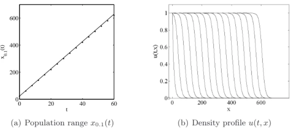
In any case, the rate of spread of the solution remains bounded. The range x_λ(t) of a solution u(t, x) of (2.1) with an EB initial datum u0 satisfying u0(x) = e−

x

10 for x ≥ 0 is

depicted in Fig. 1 (a). A very good fit for x0.1(t) is obtained with the linear function

t 7→ u−1₀ (0.1) + c(α) t. Indeed, in that case it follows from the results in Bramson (1983) that the rate of spread vλ(t) converges to c(α) as t → ∞. Convergence of the solution to

0 20 40 60 0 200 400 600 t x0.1 (t)

(a) Population range x0.1(t) (b) Density profile u(t, x)

Figure 1: (a) Population range x0.1(t) in model (2.1) with f (u) = u(1 − u) and an EB

initial datum u0 satisfying u0(x) = e− x

10 for x ≥ 0. The black dots correspond to the

approximation of x_0.1(t) by u−1₀ (0.1) + c(α) t with α = 1/10. (b) Density profile u(t, x) at successive times t = 0, 4, 8 . . . 60.

3

Fisher-KPP model with exponentially unbounded initial

data

We show here that EU initial data ineluctably lead to infinite spreading speeds and ac-celerating rates of spread. We further analyse the population range and its dependence with respect to the profile of the initial population. This analysis bears on mathematical arguments which are fully detailed in a paper by Hamel and Roques (2009) containing further mathematical results on the problem (2.1) with more general assumptions.

Consider model (2.1) with EU initial data; i.e. u₀(x) does not fulfil the condition of Definition 2.4 and is even such that u0(x) eαx → +∞ as x → +∞ for all α > 0. A

comparison principle then implies that the spreading speed is infinite. Indeed, for each 0 < α < f0_{(0), (2.1) admits a travelling wave solution u(t, x) = ϕ}

α(x − ct), moving to

the right with a constant speed c = c(α) = α + f0_{(0)/α, and satisfying ϕ}

α(x) ∼ Ce−αx

for large x. Whatever α, up to a translation xα in space, we can therefore assume that

u₀(x) ≥ ϕ_α(x + x_α) for all x ∈ R. Since ϕ_α(x + x_α− c(α)t) and u(t, x) are both solutions

to (2.1), it follows that for any α > 0,

u(t, x) ≥ ϕα(x + xα− c(α)t) for all t ≥ 0, x ∈ R.

As a consequence, the spreading speed of u is infinite. However, in most cases, it is still possible to estimate the population range: for any λ ∈ (0, K) and any ε > 0, we have

u−1₀ ³ λe−(f0(0)−ε)t ´ ≤ xλ(t) ≤ u−10 ³ λe−(f0(0)+ε)t ´ , (3.8)

for t large enough. In particular, it follows that the rate of spread v_λ(t) can be as large as we want (that is, larger than any continuous function V (t)), for large times, provided the initial condition is well chosen.

The proof of the right inequality in (3.8) is based on a comparison with an ODE model where the diffusion term has been dropped. The other inequality bears on the use of subsolutions to equation (2.1). See Appendix A for further details on the proof of these inequalities.

Let us apply the inequality (3.8) to two particular examples. First, if u0 is

logarithmi-cally sublinear for large x: u0(x) = Ce−βx

α

for large x, with C, β > 0 and 0 < α < 1, then, for any density threshold 0 < λ < K, the population range is asymptotically algebraic and superlinear in time3_: x_λ(t) ∼ µ f0₍₀₎ β ¶_1/α t1/α. (3.9)

Thus, the rate of spread vλ(t) = xλ(t)/t satisfies

vλ(t) ∼ µ f0₍₀₎ β ¶_1/α t1/α−1, (3.10)

and is asymptotically algebraic and sublinear if α > 1/2, linear if α = 1/2 and superlinear if α < 1/2.

Second, assume that u0(x) decays algebraically for large x: u0(x) = Cx−α with C > 0

and α > 0. In that case, for any 0 < λ < K, the population range xλ(t) increases

exponentially fast for large time:

ln(xλ(t)) ∼ f 0₍₀₎

α t, (3.11)

and so does the rate of spread. Though we only obtain a logarithmic equivalent in that case, the approximation of x_λ(t) by u−1₀

³

λe−f0_(0)t´

still gives good numerical results even for small times (Fig. 2 (a)).

The above discussion shows that rates of spread are qualitatively very different among models with EB and EU initial data. The shape of the solution is also different. Whereas, for EB initial data, solutions converge to travelling waves; i.e. a solution whose profile remains constant in a moving frame (Fig. 1 (b)), for EU initial data, we proved that the solutions become uniformly flat as time increases (see Fig. 2 (b)). Indeed, consider the equation satisfied by the quotient z = 1_u∂u_∂x:

∂z ∂t = ∂2_z ∂x2 + 2z ∂z ∂x+ az, with a = f 0_{(u) − f (u)/u.}

3_{By a(t) ∼ b(t), we mean that the functions a and b are equivalent as t → ∞, that is}

0 5 10 15 20 25 0 2000 4000 6000 8000 10000 t x0.1 (t)

(a) Population range x0.1(t) (b) Density profile u(t, x)

Figure 2: (a) Population range x0.1(t) in model (2.1) with f (u) = u(1 − u) and the

EU initial datum u0(x) = 1/(1 + x3). The black dots are the approximation of x0.1(t)

by u−1₀ ³

λe−f0(0)t

´

= ¡10et− 1¢1/3. (b) Density profile u(t, x) at successive times t = 0, 1, 2 . . . 27.

From the hypotheses on f the “growth term” a is nonpositive, and therefore drives the function z to 04_{. As a consequence, we have in particular:}

max x∈(−∞,+∞) ¯ ¯ ¯ ¯∂u_∂x(t, x) ¯ ¯ ¯ ¯ → 0 as t → +∞.

4

Comparison with integro-differential equations

Here, we compare the results of the preceding sections with what is known for integro-differential equations.

As for RD models, in integro-differential equations such as (Fedotov, 2001; M´endez et al., 2002; Medlock and Kot, 2003):

∂u

∂t(t, x) =

Z _+∞

−∞

j(|x − y|)u(t, y)dy − u + f (u), (4.12)

population density is given by two contributions: dispersal by the convolution kernel j and growth through the nonlinear source term f (u). Those models are the continuous-time analogue to integro-difference equations which are further discussed in Appendix B.

4_{To prove this result, in Hamel and Roques (2009), we use an additional hypothesis on u}

0: it is assumed

thatR_−∞+∞|u0

For EB kernels j, when the function f satisfies (2.2-2.3), model (4.12) is known to admit travelling wave solutions moving with a constant speed (Coville and Dupaigne, 2007). Consequently, compactly supported initial data lead in this case to bounded rates of spread.

On the other hand, as we mentioned in the Introduction, increasing rates of spread have been observed for such models with EU kernels. Medlock and Kot (2003) numerically observed a rate of spread that was linearly increasing with time, with the kernel j(s) = 1/4e−

√

|s|_{, a growth function f (u) = 10u(1 − u) and an initial density u}

0 concentrated

at one point. This is exactly what we obtain with the RD model (2.1) if we choose

u(0, x) = j(x) for large x, from equation (3.10) with α = 1/2.

A formula for the range of the solution of the linear model, where f (u) is replaced by

f0_{(0)u, was also derived by Medlock and Kot (2003). For a special type of EU kernels}

satisfying lim

s→+∞j(s)s

n_{→ 0 for all n ≥ 1, meaning that the kernel does not decrease too}

slowly, formal computations showed that xλ(t) ∼ j−1(λe−f 0_(0)t

) for large t and λ > 0. This asymptotic result is comparable to what we obtained in Section 3 for the RD model with initial datum u0(x) = j(x).

5

Spreading from cryptic refugia

The previous sections were concerned with continuous and decreasing initial data. More realistic modelling of cryptic refugia should involve initial data with fragmented support.

Such initial data can be described by the following formula:

u0(x) = 1 if x < 0 and u0(x) =

∞

X

i=0

h(x − αi)g(αi) if x ≥ 0, (5.13)

for some compactly supported function h such that h(0) = max h = 1, some increasing sequence αi→ +∞, which corresponds to the position of the refugia and a nonincreasing

function g, which describes how the population size in each refugium decreases away from the main population. It is also reasonable to assume that the sequence α_i+1− α_i

is increasing, so that the refugia get rarer and rarer as one moves away from the main population. Throughout this section, we assume that K = 1.

Let us first assume that g = 1. If, in addition, we assume that the populations in each refugium evolve independently from each other, we get that spreading occurs at the same constant rate c∗ _{from each refugium. The time at which a subpopulation}

starting from a refugium located at α_i merges with the main population (initially located in the negative region of R) is ti '

α_i− α_i−1

xλ(ti) ' αi+αi− α₂ i−1, for any λ ∈ (0, 1). Thus, the rate of spread at time ti is vλ(ti) ' c∗× µ 2 αi αi− αi−1 + 1 ¶ . (5.14)

From the assumption above, t_i increases with i; as a consequence, the rate of spread increases with time if vλ(ti) is an increasing function of i. From (5.14), we deduce that

the rate of spread is increasing if and only if

α2_i > αi+1αi−1, for i ≥ 1. (5.15)

Equivalently, the rate of spread is increasing if and only if i 7→ ln(αi) is a strictly concave

function. From (5.14) we also observe that the rate of spread tends to infinity if the ratio

αi/αi−1converges to 1.

Let us come back to the general case where g is a nonincreasing function, not necessarily equal to 1. If g is EU, it leads to fast saturation of each refugium, and the above argument should remain true. Conversely, if g is EB, a comparison principle implies that the solution of (2.1) with initial datum of the type (5.13) is smaller than the solution of (2.1) with initial datum u0 = g; thus it is impossible to have an infinite spreading speed. Hence, the above

formal analysis leads us to formulate the following conjecture: the solution to model (2.1), with an initial condition of the general form (5.13) exhibits an accelerating rate of spread and has an infinite spreading speed, if and only if g is EU and i 7→ ln(αi) is a strictly

concave function, which increments ln(α_i) − ln(α_i−1) converge to 0. These last conditions mean that the distance separating two successive refugia should not increase too fast as one moves away from the main population.

Remark 5.1. In this section, u0 is not decreasing and therefore u(t, x) is not monotone

anymore. In this case, definition 2.2 plays a critical role. If the population range were defined by xλ(t) = sup{x > 0, u(t, x) > λ}, meaning that xλ(t) is the furthest forward

po-sition where u is above the threshold λ, we would get different results. With an initial datum of the type (5.13), with g = 1 we would get x_λ(t) = +∞ for large t; on the other

hand, if g were decreasing to 0, we would get

x_λ(t) ≤ x_λ(t) ≤ sup{x s.t. u0(x) = λe−(f

0_(0)+ε)t

}

for any ε > 0 and large t. We conjecture in this case that, if g is EU, increasing rates of spread v_λ(t) = x_λ(t)/t are obtained irrespectively of the distances α_i+1− α_i.

Numerical examples

We have solved (2.1) with f (u) = u(1 − u) (thus c∗ _{= 2}p_f0_{(0) = 2), u}

0 being defined by

(5.13) with the EU function g(x) = e−√3_x

and h(x) = e− µ x x2− 1₄ ¶2 for x ∈ (−1 2,12), h(x) = 0 otherwise.

Assume first that αi = 2i. In this case ln(αi) = i ln(2) is concave, but not strictly

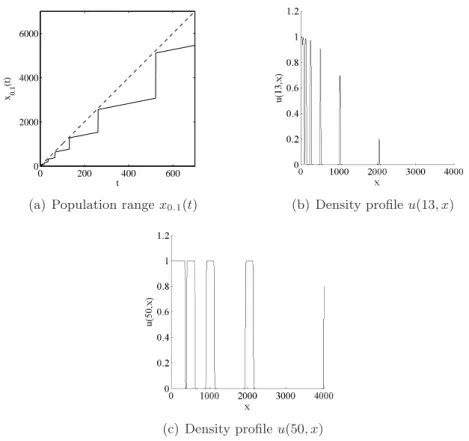
concave. Formula (5.14) indicates v_λ(t_i) ' 10, which is in good agreement with the results of the numerical computations (Fig. 3 (a)).

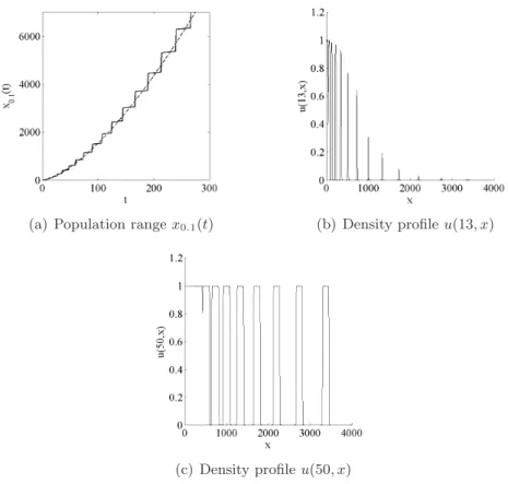
Next, assume that αi = iβ, with β > 1 (so that αi+1− αi is increasing). Then,

ln(α_i) = β ln(i) is strictly concave and ln(α_i) − ln(α_i−1) = β ln( i

i−1) → 0 as i → ∞. Thus,

following the above argument, increasing rates of spread leading to an infinite spreading speed should be obtained. With β = 3 we should have x(ti) ∼

¡_4t

i

3

¢3

2_{. Values of x(t)}

consistent with this formula were obtained (Fig. 4 (a)).

6

Discussion

For initial conditions of EB type, Fisher-KPP equations – which are archetypes of RD models – lead to finite spreading speeds. To our knowledge, the previous analyses of the spreading properties of such models were always carried out with such EB initial data. Thus RD models are usually associated with finite spreading speeds and travelling wave solutions with constant profiles.

In this paper we show that these RD models behave very differently for EB vs. EU initial data. EU initial data lead to accelerating rates of spread and infinite spreading speeds. Although they cannot be generated – in the absence of external constraints – by a simple diffusion mechanism from a localised point source, such initial data can result from previous external constraints. They should therefore be considered in modelling of recolonisation events which, by definition, follow a range retraction phase and then begin with the removal of the constraint responsible for the retraction. Because the environ-ment is heterogeneous and/or because of stochasticities, it is likely that retraction is not “perfect” and that fragments of the studied population can persist in the unfavourable habitat. These fragments act as micro-refugia and their spatial distribution governs the initial data.

These accelerating rates of spread are in fact very close to those obtained with integro-differential equations (Section 4) and integro-difference equations (Appendix B) – which traditionally model long distance dispersal events – for dispersal kernels of the same EU type than the initial condition of the RD model. Thus, RD models with EU initial data should accommodate well several data sets which were previously fitted with IDEs. For instance, the rapid spread of trees at the beginning of the Holocene (Reid’s paradox) was explained by Clark (1998) using long distance dispersal events, through integro-difference

0 200 400 600 0 2000 4000 6000 t x0.1 (t)

(a) Population range x0.1(t) (b) Density profile u(13, x)

(c) Density profile u(50, x)

Figure 3: (a) Plain line: population range x_0.1(t) of the solution u(t, x) to (2.1), with an initial density given by (5.13) and αi= 2i. Dashed line: the function t 7→ 10t. (b) and (c)

(a) Population range x0.1(t) (b) Density profile u(13, x)

(c) Density profile u(50, x)

Figure 4: (a) Plain line: population range x0.1(t) of the solution u(t, x) to (2.1), with an

initial density given by (5.13), with α_i = i3_{. Dashed line: the function t 7→}¡4t 3

¢3

2_{. (b) and}

equations with EU kernels. Our results sustain alternative explanations, such as those proposed by Skellam (1951) and later by McLachlan et al. (2005), based on the existence of cryptic refugia where the populations survived the Pleistocene glacial environment.

There are many situations where the observed rates of spread are higher than predicted with a RD model and an EB assumption on the initial population density, and where accel-eration can be found. For instance, the pine processionary moth, which is known to have a diffusive dispersal, has progressed of 86.7 km to the north of Paris between 1972 and 2004, with a notable acceleration (55.6 km) during the last 10 years (Battisti et al., 2005), leading to rates of spread higher than expected on the basis of known dispersal capabilities (females can at most travel 4 km per year [A. Roques, personal communication]). Since its ability to survive is linked to climate, it is likely that the pine processionary moth pro-gression consists in a series of colonisation-retraction-recolonisation events. Several other examples of accelerating rates of spread have been described in the literature (Hengeveld, 1989; Van den Bosch et al., 1992).

The comparison with IDEs models goes much further than rates of spread. Though not proved rigorously, flattening was numerically observed by Kot et al. (1996) for integro-difference models with fat-tailed (i.e. EU) kernels (compare our Fig. 2 (b), with Kot et al., 1996, Fig. 2, model 4). We show here that the Fisher-KPP model with EU initial data leads to the same phenomenon, in sharp contrast with what was known for EB initial data.

Mathematical statements of spreading results are generally simpler in infinite domains. However, it is noteworthy that the solution of a model like (2.1) can be approximated by the solution of the same model in a finite domain: the larger the domain, the closer the two solutions. Thus, the results of this paper remain qualitatively true in finite environments. In particular, the restriction of an EU datum to a finite interval leads to an accelerating phenomenon during a transient period whose length depends on the size of the interval. This is illustrated by our numerical results, performed in finite domains (see Appendix C). Other models have been proposed to describe accelerating rates of spread. For instance, stratified diffusion models (Shigesada et al., 1995; Shigesada and Kawasaki, 1997) where isolated colonies are founded by rare long distance dispersal events ahead of the expanding population front and expand by diffusion. For oaks, the range of which expanded rapidly at the beginning of the Holocene, these models have led to spatial genetic structures compatible with experimental data (Le Corre et al., 1997). Sharov and Liebhold (1998) also applied stratified diffusion models to the gipsy moth expansion. Patchy patterns of colonisation comparable to those obtained with stratified diffusion models can also be obtained with RD models with initial data like those introduced in Section 5.

Long distance dispersal hypothesis has often been used to explain fast spreading and ac-celerating rates of spread. It is certainly a valid explanation in several situations. However, our results show that diffusive dispersal can also very convincingly explain such patterns in a recolonisation context. The existence of colonisation-retraction-recolonisation events

is well-documented for many organisms (Gaston, 2003). Such events can for instance result from fires or climatic variations, and could lead to EU population densities. For the particular problem of tree recolonisation at the beginning of the Holocene, increasing evidence shows that cryptic refugia existed far from the main temperate refugia (Stewart and Lister, 2001; McLachlan et al., 2005; Provan and Bennett, 2008). In those cases, fast spreading and accelerating rates of spread can be obtained without the long distance hypothesis.

Appendix A: Sketch of the proof of inequality (3.8)

   du(t; x) dt = (f 0_{(0) + ε/2)u(t; x),} u(0; x) = C_εu₀(x), (6.16)

which solution is u(t; x) = Cεu0(x)e(f

0_(0)+ε/2)t

, shows that u is a supersolution (see Evans,

1998, for a precise definition) of the equation (2.1) satisfied by u, for Cε and x large

enough, for any ε > 0, provided u00₀(x)/u₀(x) → 0 as x → ∞5_{. As a consequence, for any}

ε > 0, u(t, x) ≤ Cεu0(x)e(f

0_(0)+ε/2)t

for x larger than some xε > 0 and all times t ≥ 0.

Let λ in (0, K). Since the spreading speed is infinite, after a certain amount of time,

x_λ(t) > x_ε. Thus λ = u(t, x_λ(t)) ≤ C_εu₀(x_λ(t))e(f0_(0)+ε/2)t

. As a consequence, we get, for any λ ∈ (0, K) and ε > 0, and for t large enough,

xλ(t) ≤ u−10

³

λe−(f0(0)+ε)t

´

. (6.17)

A more involved argument, based on the use of subsolutions to (2.1), like

u(t, x) = max ³ u0(x)ef 0_(0)t − M (u0(x)ef 0_(0)t )2, 0 ´ ,

for some M > 0, also enables us to give a lower bound for the population range . In fact, we claim (see Hamel and Roques, 2009, for a detailed proof) that for all ε > 0 there exists

Mε > 0 such that, for all x ∈ R and all t > 0,

u0(x)e(f

0_(0)−ε/2)t

− Mε(u0(x)e(f

0_(0)−ε/2)t

)2 ≤ u(t, x).

It follows that, when u0(x)e(f

0_(0)−ε/2)t

is small, then u0(x)e(f

0_(0)−ε)t

≤ u(t, x) for large t.

Finally, we get that for any λ ∈ (0, K) and ε > 0, and for t large enough,

u−1₀ ³ λe−(f0(0)−ε)t ´ ≤ x_λ(t). (6.18) 5_{The property u}00

0(x)/u0(x) → 0 as x → ∞ is shared by a large class of EU functions, e.g. those

satisfying, for large x, u0(x) = x−α, for α > 0, or u0= e−x

α

Appendix B: Comparison with integro-difference equations

Z _+∞

−∞

j(|x − y|)g(N_k(y))dy, with EU kernels j(s) have been studied by Kot et al. (1996), with growth functions satisfying

g(x) ≤ g0_{(0)s, for s ≥ 0.}

When the growth function g is nonlinear, expressions for the rate of spread can be delicate to obtain. Nevertheless, for EB dispersal kernels, the spreading speed was proved to be finite, and equal to the speed given by the linearised equation, where g(N_k(y)) is replaced by g0(0)Nk(y) (Weinberger, 1982).

The principle of equality between spreading speeds for a nonlinear model and its lin-earised counterpart (at 0), is referred to as the linear conjecture (Mollison, 1991). For kernels leading to infinite speeds, this conjecture is true, but does not give any informa-tion (∞ = ∞). It has however been extended, without proof, to the study of rates of spread in Kot et al. (1996), for kernels leading to such infinite speeds. The authors indeed made the assumption that the range of the solution was independent of the nonlinear part of the growth term.

Using this conjecture, for two particular kernels j1(x) = γ

2

4 e−γ|x|

1/2

and j2(x) = 1

πω2ω_+x2, Kot et al. (1996) were able to carry out explicit formulae for the population

range, starting from a Dirac (initial point source) of strength n0. Note that j2 does not

satisfy the requirement of Section 4.

The positions of the lines of level n were found to be, respectively:

x1(k) = _γ1₂ · ln[g0(0)]k + ln µ γ2n0 4n ¶¸2 and x2(k) = r ωkn0g0(0)k πn − ω2k2,

for each kernel.

To be consistent with the continuous-time models of Sections 3 and 4, we may assume that g0_{(0) = e}f0₍₀₎

. For instance, we can set

g(s) = sef (s)s for s > 0, and g(0) = 0.

We then get the equivalents x1(k) ∼ f

0₍₀₎2

γ2 k2, and ln(x2(k)) ∼ 1₂f0(0)k as k → +∞. This

exactly corresponds to the equivalents (3.9) and (3.11) obtained for the reaction-diffusion model (2.1), with initial datum u(0, x) = j(x). Thus rates of spread in integro-difference equations seem to be mainly controlled by the first dispersal event; besides, most data sets which could be fitted with integro-difference models should also be fitted with diffusion models with EU initial data.

Appendix C: numerical solution of (2.1)

The solution of the equation (2.1) in (−∞, +∞) was approximated by the solution of the same equation in a finite interval (a, b) ((−100, 2000) in the EB cases and (−100, 10000) in the EU cases) with no-flux boundary conditions: ∂u

∂x(t, a) = ∂u

∂x(t, b) = 0. Then, the

equa-tion was solved using Comsol Multiphysicsr _{time-dependent solver, using second order}

finite element method (FEM). This solver uses a method of lines approach incorporating variable order and variable stepsize backward differentiation formulas. Nonlinearities are treated using a Newton’s method.

Acknowledgements

The authors are supported by the French “Agence Nationale de la Recherche” within the projects ColonSGS (first, second, third and fifth authors), PREFERED (first and second authors) and URTICLIM (first author). The second author is also indebted to the Alexander von Humboldt Foundation for its support. The authors wish to thank the reviewers for their valuable comments on the manuscript.

References

Aronson, D. G. and H. G. Weinberger (1978). Multidimensional Non-Linear Diffusion Arising in Population-Genetics. Advances in Mathematics 30 (1), 33–76.

Battisti, A., M. Stastny, S. Netherer, C. Robinet, A. Schopf, A. Roques, and S. Lars-son (2005). Expansion of geographic range in the pine processionary moth caused by increased winter temperatures. Ecological Applications 15 (6), 2084–2096.

Booty, M. R., R. Haberman, and A. A. Minzoni (1993). The accommodation of traveling waves of Fisher’s type to the dynamics of the leading tail. SIAM Journal on Applied

Mathematics 53 (4), 1009–1025.

Bramson, M. (1983). Convergence of solutions of the Kolmogorov equation to travelling waves. Memoirs of the American Mathematical Society 44.

Brown, J. H., D. W. Mehlman, and G. C. Stevens (1995). Spatial variation in abundance.

Ecology 76 (7), 2028–2043.

Chandrasekhar, S. (1943). Stochastic problems in physics and astronomy. Reviews of

Clark, J. S. (1998). Why trees migrate so fast: Confronting theory with dispersal biology and the paleo record. American Naturalist 152, 204–224.

Clark, J. S., C. Fastie, G. Hurtt, S. T. Jackson, C. Johnson, G. King, M. Lewis, J. Lynch, S. Pacala, I. C. Prentice, E. W. Schupp, T. Webb III, and P. Wyckoff (1998). Reid’s Paradox of rapid plant migration. BioScience 48, 13–24.

Coville, J. and L. Dupaigne (2007). On a nonlocal reaction diffusion equation arising in population dynamics. Proceedings of the Royal Society of Edinburgh - A 137, 1–29. Ebert, U. and W. van Saarloos (2000). Front propagation into unstable states: universal

algebraic convergence towards uniformly translating pulled fronts. Physica D 146, 1–99. Ericsson, S., L. Ostlund, and A. L. Axelsson (2000). A forest of grazing and logging: Deforestation and reforestation history of a boreal landscape in central Sweden. New

Forests 19 (3), 227–240.

Evans, L. C. (1998). Partial differential equations. University of California, Berkeley -AMS.

Fedotov, S. (2001). Front propagation into an unstable state of reaction-transport systems.

Physical Review Letters 86 (5), 926–929.

Fisher, R. A. (1937). The wave of advance of advantageous genes. Annals of Eugenics 7, 335–369.

Friedman, A. (1964). Partial differential equations of parabolic type. Prentice-Hall, En-glewood Cliffs, NJ.

Gaston, K. J. (2003). The Structure and Dynamics of Geographic Ranges. Oxford Uni-versity Press, New York.

Hamel, F. and L. Roques (2009). Fast propagation for KPP equations with slowly decaying initial conditions. Preprint available on Arxiv http://arxiv.org/abs/0906.3164 .

Hengeveld, R. (1989). Dynamics of Biological Invasions. London: Chapman & Hall. Kametaka, Y. (1976). On the nonlinear diffusion equations of

Kolmogorov-Petrovsky-Piskunov type. Osaka Journal of Mathematics 13, 11–66.

Kay, A. L., J. A. Sherratt, and J. B. McLeod (2001). Comparison theorems and variable speed waves for a scalar reaction-diffusion equation. Proceedings of the Royal Society of

Kendall, D. G. (1965). Mathematical models of the spread of infection. In Mathematics

and Computer Science in Biology and Medicine, pp. 213–225. HMSO, London.

Kolmogorov, A. N., I. G. Petrovsky, and N. S. Piskunov (1937). ´Etude de l’´equation de la diffusion avec croissance de la quantit´e de mati`ere et son application `a un probl`eme biologique. Bulletin de l’Universit´e d’ ´Etat de Moscou, S´erie Internationale A 1, 1–26.

Kot, M., M. Lewis, and P. van den Driessche (1996). Dispersal data and the spread of invading organisms. Ecology 77, 2027–2042.

Larson, D. A. (1978). Transient bounds and time-asymptotic behavior of solutions to nonlinear equations of Fisher type. SIAM Journal on Applied Mathematics 34, 93–103. Lau, K.-S. (1985). On the nonlinear diffusion equation of Kolmogorov, Petrovsky and

Piscounov. Journal of Differential Equations 59 (1), 44–70.

Le Corre, V., N. Machon, R. J. Petit, and A. Kremer (1997). Colonisation with long distance seed dispersal and genetic structure of maternally inherited genes in forest trees : a simulation study. Genetical Research 69, 117–125.

Markoff, A. A. (1912). Wahrscheinlichkeitsrechnung. Leipzig, Germany: Teubner.

McKean, H. P. (1975). Application of Brownian motion to the equation of Kolmogorov-Petrovskii-Piscunov. Communications on Pure and Applied Mathematics 28, 323–331. McLachlan, J. S. and J. S. Clark (2004). Reconstructing historical ranges with fossil data.

Forest Ecology and Management 197, 139–147.

McLachlan, J. S., J. S. Clark, and P. S. Manos (2005). Molecular indicators of tree migration capacity under rapid climate change. Ecology 86, 2088–2098.

Medlock, J. and M. Kot (2003). Spreading disease: Integro-differential equations old and new. Mathematical Biosciences 184 (2), 201–222.

M´endez, V., T. Pujol, and J. Fort (2002). Dispersal probability distributions and the wavefront speed problem. Physical Review E 65 (4), 1–6.

Mollison, D. (1972). Possible velocities for a simple epidemic. Advances in Applied

Prob-ability 4, 233–257.

Mollison, D. (1977). Spatial contact models for ecological and epidemic spread. Journal

of the Royal Statistical Society: Series B 39, 283–326.

Mollison, D. (1991). Dependence of epidemic and population velocities on basic parame-ters. Mathematical Biosciences 107, 255–287.

Pearson, K. and J. Blakeman (1906). Mathematical contributions of the theory of

evolu-tion. A mathematical theory of random migraevolu-tion. Drapersi Company Research Mem.

Biometrics Series III, Dept. Appl. Meth. Univ. College, London.

Provan, J. and K. D. Bennett (2008). Phylogeographic insights into cryptic glacial refugia.

Trends in Ecology & Evolution 23, 564–571.

Reid, C. (1899). The origin of the British flora. London : Dulau & Co.

Romagni, J. G. and C. Gries (2000). Post-fire recolonization of dominant epiphytic lichen species on Quercus hypoleucoides (Fagaceae). American Journal of Botany 87, 1815– 1820.

Sharov, A. A. and A. M. Liebhold (1998). Model of slowing the spread of the gypsy moth (lepidoptera: Lymantriidae) with a barrier zone. Ecological Applications 8, 1170–1179. Shigesada, N. and K. Kawasaki (1997). Biological invasions: theory and practice. Oxford

Series in Ecology and Evolution, Oxford: Oxford University Press.

Shigesada, N., K. Kawasaki, and Y. Takeda (1995, Aug). Modeling Stratified Diffusion in Biological Invasions. American Naturalist 146 (2), 229–251.

Skellam, J. G. (1951). Random dispersal in theoretical populations. Biometrika 38, 196– 218.

Stewart, J. R. and A. M. Lister (2001). Cryptic northern refugia and the origins of the modern biota. Trends in Ecology & Evolution 16, 608–613.

Uchiyama, K. (1978). The behaviour of solutions of some non-linear diffusion equations for large time. Journal of Mathematics of Kyoto University 18 (3), 453–508.

Van den Bosch, F., R. Hengeveld, and J. A. J. Metz (1992). Analysing the velocity of animal range extension. Journal of Biogeography 19, 135–150.

Weinberger, H. F. (1982). Long-time behavior of a class of biological models. SIAM