Computational aspects of ductile crack growth in three dimensions

Computational Aspects of Ductile Crack Growth

in Three Dimensions

by

Vaibhaw Vishal

Bachelor of Technology in Mechanical Engineering,

Indian Institute of Technology, Bombay, India (2000)

Submitted to the Department of Mechanical Engineering

in partial fulfillment of the requirements for the degree of

Master of Science in Mechanical Engineering

at the

MASSACHUSETTS INSTITUTE OF TECHNOLOGY

MASSACHUSETTS INST11TUTE

OFTECHNOLOGY

JUL

16,2003

LIBRARIES

June 2003

©

Massachusetts Institute of Technology 2003. All rights reserved.

A uthor ...

...

Department of Mechanical Engineering

Vy 23, 2003

Certified by...

David M. Parks

Professor of Mechanical Engineering

esis Supervisor

Accepted by ...

..

r

Ami

Computational Aspects of Ductile Crack Growth in Three

Dimensions

by

Vaibhaw Vishal

Submitted to the Department of Mechanical Engineering on May 23, 2003, in partial fulfillment of the

requirements for the degree of

Master of Science in Mechanical Engineering

Abstract

Ductile crack growth can occur in many engineering applications, such as penetrating cracks in pressure vessels. Simulations of ductile crack growth are performed on a 3-D open-bend specimen. Two different finite element schemes namely, implicit finite element scheme and explicit finite element scheme are used to perform the simulations. Various type of meshes consisting of first-order and second-order tetrahedral elements (along with/without a brick or prism elements layer next to the crack-containing-plane) are used. Explicit finite element scheme takes about nine times higher cpu-time (on a Compaq AlphaStation DS20E, two processors at 667MHz each). Load-displacement curves show a steeper drop off after peak value when simulations are performed with explicit finite element scheme compared to when simulations are performed with implicit finite element scheme.

Thesis Supervisor: David M. Parks

Acknowledgments

I want to express my deep sense of gratitude to my advisor, Prof. D.M.Parks, for his invaluable guidance and constant encouragement throughout this work. I have learnt a lot while working with him and have enjoyed interacting with him. I would also like to thank Prof. F.A.McClintock for his insightful guidance into the field of fracture mechanics.

A want to thank my fellow graduate students, Dora, Rajdeep, Nuo, Nici, Jin, Yin, Hang, Ekrem, Ted, for their support. A special thanks to Ray Hardin for handling all the administrative works.

I would also like to thank my friends Sachin and Shweta for making a homely at-mosphere in Boston.

Support for this research was provided by the D.O.E. under grant number DE-FG02-85ER13331 to MIT.

Contents

1 Introduction 11

1.1 Motivation and Application . . . . 11

1.2 Organization of Present Work . . . . 12

2 Finite Element Modeling 16 2.1 GTN Failure M odel . . . . 16

2.2 Elements Used in Simulations . . . . 22

2.2.1 Advantages and Disadvantages of Various Tetrahedral Elements 23 2.3 Modified Second-Order Tetrahedral Element . . . . 24

2.4 Issues in Using C3D10M With the GTN Failure Model . . . . 26

2.5 Procedure for Adding Brick-Element Layer to a surface C3D10M Ele-m ent Layer . . . . 27

3 Finite Element Results with Abaqus/Standard 30 3.1 M esh Details . . . . 30

3.2 M aterial M odel . . . . 32

3.3 Comparison of Load-Displacement Curves . . . . 32

3.4 Void Volume Fraction Evolution for Different Meshes . . . . 33

3.5 CPU Time Comparison . . . . 34

4 Finite Element Results with Abaqus/Explicit 51 4.1 M ass Density Scaling . . . . 51

4.3 Comparison of Various Meshes . . . . 55

5 Summary and Conclusions 70

5.1 Future W ork . . . . 73

List of Figures

1-1 A typical specimen. (a) Full 3-D geometry. (b) 2-D idealization (plane strain ). . . . . 14 1-2 2-D idealization of pressure vessel showing a longitudinal penetrating

crack. ... ... 15

2-1 True stress-strain curve from ASTM standard compression test on A572 Gr. 50 steel (taken from [1]). . . . . 17 2-2 Effect of void volume fraction on yield surface (schematic). . . . . 19 2-3 Uniaxial behavior of a porous material against fully dense material

(schem atic). . . . . 20 2-4 Modified second-order tetrahedral element (C3D1OM). . . . . 24 2-5 Tetrahedral element (C3D1OM) divided into four hexahedral elements. 25 2-6 Brick elements attached to tetrahedral elements. . . . . 28 2-7 Typical mesh detail showing a layer of brick elements attached to

C3D1OM elements. . . . . 29

3-1 Specimen geometry (a) Full geometry. (b) Quarter geometry which is modeled in finite element method. All dimensions are in mm. .... 35 3-2 Schematic of void nucleation, growth, and coalescence in ductile metals

(taken from [2]). . . . . 36 3-3 Details of mesh-1. (a) Isometric view. (b) Zoomed isometric view. . 37

3-4 Details of mesh-2. (a) Isometric view. (b) Zoomed isometric view. . 39

3-5 Details of mesh-3. (a) Isometric view. (b) Zoomed isometric view. . 41

3-7 Load-displacement curves. . . . . 45 3-8 Contours of void volume fraction plotted on the crack-containing-plane

(at a load-point displacement of 10.4 mm), obtained with (a) Mesh-1. (b) M esh-2. . . . . 46 3-9 O-33 Contours of stress (0o33) plotted on the crack-containing-plane (at

a load-point displacement of 10.4 mm), obtained with (a) Mesh-1. (b) M esh-2. . . . .... .... ... .... . . . ... . . .... . 48 3-10 Brick elements attached to a tetrahedral element. . . . . 50

4-1 Kinetic energy and total deformation energy curves for (a) mesh-1, (b) mesh-3, and (c) mesh-4. . . . . 57 4-2 Material model distribution in finite element mesh (schematic). (a)

Case-1: GTN model with element failure restricted to only one layer next to the crack-containing-plane, classical plasticity in the rest of the mesh. (b) Case-2: GTN model throughout the mesh, element failure restricted to only one layer next to the crack-containing-plane. (c) Case-3: GTN model with element failure throughout the mesh. . . . . 58 4-3 Load-displacement curves obtained with mesh-3 for the three different

cases of material model distribution. . . . . 59 4-4 Contours of normal stress (O-33) obtained with mesh-3 (view of the

crack-containing-plane at a load-point displacement of 10.5 mm ). (a) Case-1: GTN model with element failure in only one layer next to the crack-containing-plane, classical plasticity in the rest of the mesh. (b)

Case-2: GTN model throughout the mesh, element failure in only one layer next to the crack-containing-plane. (c) Case-3: GTN model with element failure throughout the mesh. . . . . 60

4-5 Contours of void volume fraction obtained with mesh-3 (isometric view at a load-point displacement of 10.5 mm). (a) Case-1: GTN model with element failure in only one layer next to the

crack-containing-plane, classical plasticity in the rest of the mesh. (b) Case-2: GTN model throughout the mesh, element failure in only one layer next to the crack-containing-plane. (c) Case-3: GTN model with element failure throughout the mesh. . . . . 61 4-6 Contours of equivalent plastic strain obtained with mesh-3 (isometric

view at a load-point displacement of 10.5 mm). (a) Case-1: GTN model with element failure in only one layer next to the crack-containing-plane, classical plasticity in the rest of the mesh. (b) Case-2: GTN model throughout the mesh, element failure in only one layer next to the crack-containing-plane. (c) Case-3: GTN model with element failure throughout the mesh. . . . . 62 4-7 Contours of void volume fraction obtained with mesh-3 (view of the

crack-containing-plane at a load-point displacement of 10.5 mm). (a) Case-1: GTN model with element failure in only one layer next to the crack-containing-plane, classical plasticity in the rest of the mesh. (b) Case-2: GTN model throughout the mesh, element failure in only one layer next to the crack-containing-plane. (c) Case-3: GTN model with element failure throughout the mesh. . . . . 63 4-8 Contours of void volume fraction, at various load-point-displacement,

obtained with mesh-3, case-1. (a) at a load-point displacement of 5.5 mm. (b) at a load-point displacement of 8.8 mm. (c) at a load-point displacement of 10.5 mm . . . . 64 4-9 Contours of void volume fraction, at various load-point-displacement,

obtained with mesh-3, case-2. (a) at a load-point displacement of 5.25 mm. (b) at a point displacement of 8.8 mm. (c) at a load-point displacement of 10.5 mm. . . . . 65

4-10 Contours of void volume fraction, at various load-point-displacement, obtained with mesh-3, case-3. (a) at a load-point displacement of 5.25 mm. (b) at a point displacement of 8.8 mm. (c) at a load-point displacement of 10.5 mm. . . . . 66 4-11 Contours of normal stress (o33) at a load-point displacement of 10.5 mm

obtained with (a) mesh-3. (b) mesh-4. . . . . 67 4-12 Contours of void volume fraction, at various load-point-displacements,

obtained with mesh-4; GTN model with element failure throughout the mesh. (a) at a load-point displacement of 5.0 mm. (b) at a load-point displacement of 8.0 mm. (c) at a load-point displacement of 10.0 mm. 68 4-13 Load-displacement curves obtained with mesh-3 and mesh-4. . . . . . 69

5-1 Load-displacement curve obtained with mesh-3 using Abaqus/Standard and Abaqus/Explicit. . . . . 74 5-2 Load-displacement curve obtained with mesh-4 using Abaqus/Standard

and Abaqus/Explicit. . . . . 75 5-3 Contours of void volume fraction plotted on the crack-containing-plane

for mesh-3 (at a load-point displacement of 10.5 mm). (a) Simula-tion performed with Abaqus/Standard. (b) SimulaSimula-tion performed with Abaqus/Explicit. . . . . 76 5-4 Contours of -33 plotted on the crack-containing-plane for mesh-3,

List of Tables

2.1 Flow stress values at different plastic strain levels for A572 Gr. 50 steel (taken from [1]) .. . . . . 2.2 Parameters used in the Gurson-Tvergaard-Needleman model. . . . . .

3.1 CPU run-time comparison for various meshes. . . . .

4.1 CPU run-time comparison for various cases and meshes. . . . . 18 22

34

56

Chapter 1

Introduction

1.1

Motivation and Application

The resistance of ductile metals to stable crack extension strongly affects the safety and reliability of critical engineering structures. Fully-plastic crack growth or ductile crack growth can occur in many engineering applications such as long part-through cracks in tension in wide plates, penetrating cracks in pressure vessels, ship hulls etc. For many steels and aluminum alloys, a large increase in plastic deformation ahead of the crack front during the first few millimeters of (stable) crack extension permits increase in the crack driving force (e.g., the J-integral) to levels several times the values present at the initiation of growth.

At the micro-scale, crack growth commonly involves a mechanism of void nucle-ation, growth, and coalescence driven by the plastic strain field and (tensile) mean stress ahead of crack front. However, the macroscopic geometry and loading mode, combined with material flow properties, largely determines the level of mean stress and plastic strain attainable along the crack front. To better understand this complex interaction and to provide reliable prediction of crack growth resistance, robust and efficient computational tools which couple macro-scale features with realistic models of the micro-scale growth mechanisms are required.

[3,

[7],

Simulations of ductile crack growth can be performed using the finite element method. In many specimens (such as shown in Fig. 1-1), it is often attractive to use the 2-D idealization (Fig. 1-1) of the problem to perform the simulation, as the latter requires much less computational effort, compared to modeling the 3-D specimen. Simulating ductile crack growth using a 2-D idealization has a major

disadvantage; namely, it can not capture crack tunneling behavior which occurs in reality. This disadvantage (of 2-D idealizations) may result in predicting unstable crack growth when the crack may actually be stable. An experiment performed by INEEL shows a similar result. In the experiment, hydro test on a cylindrical pressure vessel containing a long, nearly constant depth longitudinal part-through crack was performed, a simulation based on a 2-D model of the vessel (Fig. 1-2) predicted a violently unstable crack growth whereas in experiment the pressure vessel leaked stably. Thus, it is important to simulate ductile crack growth in 3-D rather than only in its 2-D idealization.

Simulating ductile crack growth in 3-D specimens requires very high computa-tional effort. To solve the problem in a reasonable time, with desired accuracy, it is important to wisely choose the finite element scheme along with the type of elements to be used in the simulations. It is important to understand the relative advantages and disadvantages of each finite element scheme (e.g., implicit static scheme versus explicit dynamic scheme). It is also important to understand the relative merits of available elements such as, tetrahedral versus brick elements, second-order versus first-order elements, and how these elements perform within each of the finite element

schemes.

1.2

Organization of Present Work

Ductile crack growth is simulated in a 3-dimensional, 4-point loading open-bend spec-imen using an implicit finite element scheme (Abaqus/Standard) and an explicit finite element scheme (Abaqus/Explicit). Various types of elements are used. Chapter two

describes the Gurson-Tvergaard-Needleman (GTN) material model, which is used to simulate the growth of voids and resultant material softening. The material proper-ties and the parameters of the GTN model used in the simulations are also given. This chapter further discusses the various types of elements available for simulations and discusses advantages and disadvantages of each. This chapter also shows how a brick-element-layer can be attached to the second-order modified tetrahedral elements (C3D1OM elements of Abaqus).

Chapter three gives the specimen geometry and dimensions; it also provides all the meshes which are used in the simulations. The open-bend simulations performed on these meshes using Abaqus/Standard are presented in this chapter. The load-displacement curves obtained from all the meshes are compared and discussed. The void volume fraction values, equivalent plastic strain values, and stress values for all the meshes are compared using contour plots. The cpu-time required for all the meshes are also compared.

Chapter four presents the results obtained with Abaqus/Explicit. Various types of material modeling are used in this chapter, such as using isotropic hardening Mises-based plasticity away from the crack-containing-plane and the GTN model next to the crack-containing-plane. The load-displacement curves obtained with these differing material models are compared. The void volume fraction values and crack advance patterns are compared and discussed through contour plots. The cpu-time required

for each of them is also tabulated.

Finally, chapter five summarizes the results and provides interpretations of the differences between the results obtained from the two finite element schemes. It also gives recommendations for future work in this area.

Crack

(a)

Crack

(b)

Figure 1-1: A typical specimen. (a) Full 3-D geometry. (b) 2-D idealization (plane strain).

Internal Pressure Applied

Figure 1-2: 2-D idealization of pressure vessel showing a longitudinal penetrating crack.

Chapter 2

Finite Element Modeling

Finite element simulations of ductile crack growth are performed on 4-point loading open-bend specimen with different meshes. The details of the specimen are given in the next chapter. The material properties used in all the simulations are of A572 Gr. 50 steel. The Youngs's modulus of this steel is taken as E = 207GPa and the Poisson's ratio is taken as v = 0.30. The strain hardening (Table 2.1) of this material

is calculated from the true stress-strain curve shown in Fig. 2-1, obtained from an ASTM standard compression test [1] on A572 Gr. 50 steel.

The failure model used in the simulations is the Gurson-Tvergaard-Needleman (GTN) porous plasticity model for void-containing materials. This model was first proposed by Gurson [3] and later modified by Tvergaard and Needleman. The model is described below.

2.1

GTN Failure Model

The Gurson model analyzes plastic flow in a void-containing material by averaging the effect of voids throughout the material. The amount of voids is quantified by using porosity (or void volume fraction),

f,

0O Cf) 900 800 700 600 500 400 300 200 100 0 0 0.1 0.2 0.3 0.4 0.5 0.6 0.7 True Strain

Figure 2-1: True stress-strain curve from ASTM standard compression test on A572 Gr. 50 steel (taken from [1]).

I I I I I

Flow Stress, S (MPa) Plastic Strain, egm 3.53E+2 0 4.76E+2 0.009406 5.24E+2 0.019175 5.55E+2 0.029022 5.79E+2 0.038906 5.99E+2 0.048811 6.16E+2 0.058730 6.27E+2 0.068675 6.36E+2 0.078633 6.44E+2 0.088595 6.51E+2 0.098561 6.57E+2 0.108530 6.63E+2 0.118501 6.69E+2 0.128474 6.74E+2 0.138449 6.79E+2 0.148425 6.83E+2 0.158403

Table 2.1: Flow stress (taken from [1]).

of mean stress, Urn, to tensile flow strength, S, is plotted along the X-axis, and the ratio of Mises stress, req, to tensile flow strength, S, is plotted along the Y-axis (only positive portions of or/S and ueq/S axes are shown because in the GTN model, yield surface, <D, is an even function of Ur/S and aUq/S). The figure shows that, for

f

f

the porosity increases, the yield surface shrinks in size; i.e., yielding occurs at lower values of stress. Figure 2-3 compares the uniaxial stressing behavior of a porous metal with initial void volume fraction fo against a fully dense (void volume fraction = 0) perfectly plastic material. In this figure, true strain is plotted along the X-axis and true stress is plotted along the Y-axis. The figure shows that porous metal yields at a lower value of stress (both in tension and compression), compared to fully-dense metal. Also in compression, the porous material hardens due to closing of the voids, while in tension, it softens due to nucleation and growth of voids.

ceq S

f 0

(Mises)

S compression (fO)-f0 =0 (Mises) tension (fO) C, -s Figure 2-3: (schematic).

In the Gurson model, the yield surface is given by,

=(e) 2 _{+ 2f cosh 3 [1 + f2= 0, (2.1)}

where ueq is Mises stress, S is tensile flow strength of fully dense matrix at the current level of matrix work hardening, urn is mean hydrostatic stress, and f is void volume fraction. Tvergaard and Needleman [4], [5], [6] modified the above model by introducing two dimensionless parameters, qi and q2, and by replacing

f

f*,

f if

f

fc,7

f*

+ f -_'7 if fc < f < fF,

where

fc

S= () 2±+ 2qif* cosh 3q2m - [1 + (qi f*)2 = 0. (2.3) This addition of qi and q2 amplifies the effect of hydrostatic stress on yielding, and

the replacement of

f

f*

f

fc

To calculate the evolution of

f,

f

f

where fnucieation is the rate of change in void volume fraction due to the creation of

new voids, and jgrowth is due to the rate of growth of existing voids. The rate of nucleation of new voids is assumed to be plastic-strain-controlled and is given by

SfN {2 pN

fnucleation =2r exp- 2

J

the mean and standard deviation of normal distribution of void nucleation strain, and fN is the volume fraction of nucleating voids. The growth of existing voids is based on conservation of mass, and is given by

fgrowth= (1 - f) it, (2.6)

where P is rate of volumetric plastic strain. The plastic strain increment is given by the normality flow rule

P = A ,4 (2.7)

where cxj are the components of the Cauchy stress tensor. During plastic flow the parameter A is obtained from the consistency condition <> = 0. The hardening of fully-dense matrix material is given as a function of equivalent plastic strain in fully

dense matrix by (Table 2.1),

S = S (&eqm). _(2.8)

The evolution of the equivalent plastic strain in the matrix is given by the equivalence of plastic work

(1

f)

The numerical values of void nucleation parameters EN, SN and fN, as well as for the initial void volume fraction, fo, and the material failure parameters,

f,

fo eN SN IfN f fF q, q2 0.002 0.32 0.10 0.03 0.15 0.25 1.5 1.0

Table 2.2: Parameters used in the Gurson-Tvergaard-Needleman model.

2.2

Elements Used in Simulations

The quality of 3-D meshes generated with tetrahedral elements has been consistently improving over the past decade. Generating a 3-D mesh is easy and fast with

tetra-hedral elements. Unfortunately, mesh generation with brick elements is not so well developed. For the present work tetrahedral-element-based meshes are used. Various types of tetrahedral elements are available in Abaqus, and each has some advantages and disadvantages, which are described below.

2.2.1

Advantages and Disadvantages of Various Tetrahedral

Elements

* 4-noded first-order tetrahedral element (C3D4); these elements are com-putationally efficient and fast as they require only one integration point per element, but these elements have problems of volumetric and shear locking [10]. Very fine meshes are often needed for good accuracy if these elements are used

in a simulation.

" 10-noded second-order tetrahedral element (C3D1O); being second-order elements, they have four integration point per element, and so require more com-putational effort per element. They give good accuracy with finite deformation. However these elements are not appropriate for contact problems because in uniform pressure situations the contact forces are non-uniform at the corner and mid-side node (corner nodes carry zero nodal forces) [10]. Further, these elements may exhibit significant volumetric locking when incompressibility is approached.

" 10-noded modified second-order tetrahedral element (C3D10M); these elements exhibit minimal volumetric and shear locking and provide robustness and convergence for contact simulations, but are computationally expensive, especially in explicit dynamics simulations, because they require four integration points per element and also have linear multi-point constraints applied to some of its nodes. With these elements, relatively coarse meshes can be used for

2.3

Modified Second-Order Tetrahedral Element

The modified second-order tetrahedral element (C3D1OM) is shown in Fig. 2-4.

111

Figure 2-4: Modified second-order tetrahedral element (C3D1OM).

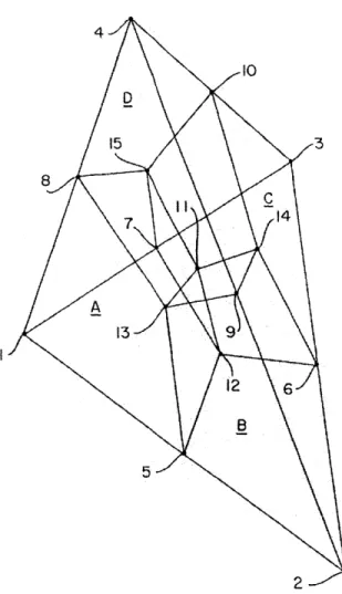
This element has ten user-defined nodes (node numbers 1-10). Node numbers 1-4 are vertex nodes, and node numbers 5-10 are mid-edge nodes. In these elements Abaqus adds five internal nodes (node numbers 11-15, which are invisible to user), and divides each tetrahedral element into four hexahedral elements, as shown in Fig. 2-5. These hexahedral sub-elements use a uniform strain formulation as developed in [11]; hourglass control is applied to the assembly of hexahedral elements and is described in [12].

The coordinates of node 11, which is a mid-body node, are given by

4 fO 01 5 3 13 9 B 2

where Atet = -0.006803281, Btet = 0.162131146, and Xi are the coordinates of the

ith node. This mid-body node is free to move; i.e., three degrees of freedom, one in each Cartesian direction, are added to the system by the addition of this node. The initial coordinates of nodes 12-15, which are mid-face nodes, are given by,

X12 = Atri(X1 + X2 + X3) + Btri(X5 + X6 + X7),

X₁₃ = Atri(XI + X2 + X4) + Btri(X5 + X8 + X9),

(2.11)

X14- Atri(X 2 + X3 + X4) + Btri(X6 + X9 + X10),

X15= Atri(Xi + X3 + X4) + Btri(X 7 + X8 + X10),

where Atri = -1/15, Btri = 2/5, and Xi are the coordinates of the ith node. These

nodes are constrained to move in a specific way; e.g., node 12, which is on the face formed by nodes 1, 2, 3, 5, 6, and 7, is constrained to move according to

U12 =Atri(Ui + u2 + u3) + Btri(U5 + U6 + u7) (2.12)

where Ati = -1/15 and Btri = 2/5, and ui is the displacement of the ith node. Node numbers 13-15 are also constrained to move in a similar fashion. Further details about this element are given in [12].

2.4

Issues in Using C3D10M With the GTN

Fail-ure Model

Many metals which fail by a void growth mechanism often display a macroscopically planar fracture surface. Very little or no void growth is observed away from the crack-containing plane [13]. Since many calculations are involved in finding the yield surface and void growth rate in the GTN failure model, it may be computationally inefficient to use the GTN model throughout the mesh. Therefore, in some of the simulations, to reduce computational effort, the GTN failure model is used in only one element layer (attached to the crack plane), and classical plasticity is used away from this layer. Using this type of modeling will have the disadvantage that we will

never know if the crack "wanted" to turn off-plane in a shear-band.

To limit fracture to the crack-containing plane, a layer of brick elements is attached to the tetrahedral element layer. The procedure for adding the brick element layer is described in the next section. Similar approaches of using two different types of elements in a mesh, one attached to the crack plane, and a different one away from it, have been used by many researchers; e.g., Xia & Shih [14] used computational cells near the crack plane for modeling ductile crack growth and Ortiz & Pandolfi [15] used irreversible cohesive elements near the crack plane for 3-D crack propagation analysis.

2.5

Procedure for Adding Brick-Element Layer to

a surface C3D10M Element Layer

To add brick elements on a face of a C3D1OM element, first, an additional node (node 16) is defined (Fig. 2-6) with the coordinates given by

X16 - Atri(Xi + X2 + X3) + Btri(X5 + X6 + X7) (2.13)

where Atrj = -1/15, Btri = 2/5, and Xi is the position vector of the ith node. This node (node 16) has the same coordinate as the Abaqus added internal node (node 12) of Fig. 2-4. This newly-added node is constrained to move according to the equation

U_{1 6} Atri (U + u2 + u3) + Btri(u5 + u6 + u7) (2.14)

where Atri = -1/15 and Btri = 2/5, and ui is the displacement of the ith node. Constraining this newly-added node in the way described above makes sure that this node coincides all the time with the moving, but hidden node (node 12 of Fig 2-4) of Abaqus.

To complete the formulation of the brick element layer, new nodes are defined at a height h below each node of the face of the tetrahedra (Fig 2-6), and the

newly-Face of

tetrahedral element

16

6

h

5

3 added

brick elements

-

--added node (node 16). This way, three cylindrical brick elements can be attached to one face of each tetrahedral element. A Fortran code is written to attach a layer of brick elements to a given C3D1OM element mesh. The code is given in appendix A. Figure 2-7 shows a mesh detail in which a layer of brick elements is attached to C3D1OM elements.

C3D1OM elements Brick elements

Figure 2-7: Typical mesh detail showing a layer of brick elements attached to C3D1OM elements.

Chapter 3

Finite Element Results with

Abaqus/Standard

Finite element simulations are performed using the commercially-available finite ele-ment software Abaqus/Standard, Versions 5.8, 6.1, and 6.3 [16, 17, 18]. The specimen geometry is shown in Fig. 3-1. A quasi-static analysis is performed in which a dis-placement, u, is applied on the center of top rollers while the bottom rollers are held fixed. Because of symmetry only one-quarter of the specimen is meshed with finite elements. In all the simulations of this chapter, the rollers are assumed to be fric-tionless and rigid. Four different meshes, mesh-1, mesh-2, mesh-3, and mesh-4, are considered. The details of these meshes are given below.

3.1

Mesh Details

Element size and mesh design play an important role in simulating ductile crack growth ([19],[20]). On the physical level, ductile fracture occurs because of void nu-cleation, growth and coalescence. Once voids nucleate (around second phase particles or inclusions), further plastic strain and hydrostatic stress causes them to grow and eventually coalesce. Figure 3-2 schematically illustrates the growth and coalescence mechanism of micro-voids. If the initial void volume fraction of voids is low (less than 10%) [2], each void can be assumed to grow independently; upon further growth,

neighboring voids interact. Plastic strain gets concentrated along a sheet of voids, and local necking instability develop. To capture this local instability, element size to be used in the finite element calculations should be of the order of inter-particle spacing (spacing between large inclusions). This way the element size provides the otherwise missing physical length-scale over which continuum damage occurs.

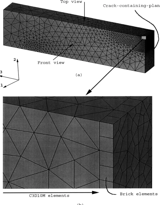
Mesh-1 is shown in Fig. 3-3; part (a), and part (b) of this figure show the isometric view of the specimen mesh, whereas parts (c), (d), and (e) show front view, top view, and a view of the crack-containing-plane, respectively. In this mesh C3D1OM elements are used away from the crack-containing-plane, and a 0.3 mm-thick layer of 8-noded brick elements (C3D8) is used on the crack-containing-plane. These brick elements are attached to the C3D1OM elements in the manner described in the previous chapter. The brick-layer can be seen in zoomed isometric view, as shown in Fig. 3-3(b). The number of (user) nodes and the number of elements in this mesh are 41,783 and 27,881, respectively. If we define the effective element size on the crack-containing-plane by the equation,

4 x Area of an element-face on the crack-containing-plane Perimeter of the element-face on crack-containing-plane '

the effective element size for this mesh is 0.23 mm.

Mesh-2 is shown in Fig. 3-4. In this mesh, again C3D1OM elements are used (away from the crack-containing-plane), along with a 0.3 mm-thick brick-element layer (on the crack-containing-plane). The number of (user) nodes and the number of elements in this mesh are 53,346 and 35,930, respectively. The only difference between mesh-1 and mesh-2 is in their number of nodes and elements. Mesh-2 is about 25% denser than mesh-1. The effective element size for this mesh is 0.20 mm.

In mesh-3 (Fig. 3-5), instead of using C3D1OM elements away from the crack-containing-plane, first-order 4-noded tetrahedral elements (C3D4) are utilized. A layer of 6-noded triangular prism elements (C3D6) is attached to these tetrahedral elements; the thickness of this prism layer is 0.3 mm. Displacement compatibility between C3D4 elements and C3D6 elements is ensured by extruding C3D6 elements

from the base of C3D4 elements. The number of nodes and the number of elements in this mesh are 16,174 and 78,173, respectively. The effective element size for this mesh is 0.23 mm.

In mesh-4 (Fig. 3-6), first-order 4-noded tetrahedral elements (C3D4) are used throughout the mesh. The number of nodes and the number of elements in this mesh are 15,030 and 75,996, respectively. The effective element size for this mesh is 0.23 mm.

3.2

Material Model

In all the simulations, the matrix hardening of Fig. 2-1, along with the Gurson pa-rameters of Table 2.2 are used. Since Abaqus/Standard does not easily accommodate element deletion (failure), the GTN material model without element failure is used. In this chapter, the GTN material model is used throughout the mesh. Later, for comparison purposes, some simulations are performed with the GTN material model in one layer next to the crack-containing-plane, and classical plasticity in the rest of the mesh. It will be noted that using the GTN material model throughout the mesh does not significantly increases the CPU time.

3.3

Comparison of Load-Displacement Curves

Figure 3-7 compares load displacement curves for all the meshes. Mesh-1 and mesh-2 give almost identical displacement curves, but mesh-3 shows a lower load-displacement curve than that of the other meshes. This is because mesh-3 has a higher value of void volume fraction on the crack-containing-plane than other meshes (Fig. 3-8). Since elements soften and carry less load at high void volume fraction values, therefore the load-displacement curve for mesh-3 is lower than the load-displacement curves of other meshes.

Since the simulations in this chapter are performed using Abaqus/Standard, ele-ments on the crack-containing-plane never fail and continue to carry load in

direction-3. This can be seen in Fig. 3-9, which show contours of -33 on the crack-containing-plane for all the meshes. The figure shows positive values of O-33 in the crack-growth

region. Some elements on the crack-containing-plane, which should have actually failed (because of high value of void volume fraction) and carry no load, are carrying load in direction-3, leading to a higher load-displacement curve. This condition is further worsened because of the long "moment arm" of these elements. To resolve this problem of overestimating the load-displacement curve and thereby falsely indi-cating more stability, in the next chapter, another finite element software program, Abaqus/Explicit is used, which accommodates element failure easily.

3.4

Void Volume Fraction Evolution for Different

Meshes

Figures 3-8 (a), (b), (c), and (d) show contours of void volume fraction for mesh-1, mesh-2, mesh-3, and mesh-4, respectively. The contours are shown on the crack-containing-plane for a load-point displacement of u =10.4 mm. Lower values of void volume fraction are observed in mesh-1 and mesh-2, compared to mesh-3. This is because the evolution of void volume fraction depends upon plastic strain increments (eq. 2.4, 2.5, and 2.6), and plastic strain increments would be smaller in a brick element of mesh-1 and mesh-2, compared to a prism element of mesh-3, as explained

below.

Consider brick-element 1 shown in Fig. 3-10. The plastic strain increment of this element will depend on the displacement increment of node 3 (because node 16 is constrained to move according to eq. 2.14), which is far away from crack front, and therefore has a small value of displacement increment. This in turn gives a low value of plastic strain increment in element 1. Whereas no such constraint exists in prism elements of mesh-3, and hence lower void volume fraction values are observed in mesh-1 and mesh-2, compared to that observed in mesh-3.

0.20 mm (as mentioned in section 3.1, which is calculated based on the area and perimeter of a brick element); rather, it is 0.36 mm and 0.33 mm, respectively (which is calculated based on the area and perimeter of a C3D1OM element-face just above the brick layer). Because of this higher effective element size, lower void volume fraction values are observed in mesh-1 and mesh-2, compared to that observed in mesh-3.

Further, poor contours of void volume fraction are observed in mesh-4. This is because mesh-4 contains only C3D4 elements on the crack-containing-plane. These elements have three nodes on the crack-containing-plane and only one node away from it. When these element have softened because of void growth, they become very compliant and essentially carry uniaxial load (low-triaxiality) in direction three. Because of low-triaxiality, the volumetric plastic strain increment is smaller, which results in slower void growth (eq. 2.6).

3.5

CPU Time Comparison

The CPU-time (on a Compaq Alpha Station DS20E, two processors at 667MHz each) for all the simulations are tabulated in Table 3.1. Mesh-1 and Mesh-2, which utilize second-order modified tetrahedral elements with a brick layer, result in significantly higher CPU-time, compared to that required for mesh-3 and mesh-4, which utilize first-order tetrahedral elements.

Mesh No. of nodes No. of elements CPU Time Mesh-1 41783 27881 50 hours 44 minutes Mesh-2 53346 35930 84 hours 28 minutes Mesh-3 16174 78173 10 hours 40 minutes

Mesh-4 15030 75996 9 hours 56 minutes

- -~~Jnu-T-~ -- - -= ---. ~--- -- -~---ii (applied) P/2 d=38.1 P/2 (calculated) D = 25.4 B = 25.

1

Front symmetry plane (fixed in direction-2)

(b)

Figure 3-1: modeled in

Specimen geometry (a) Full geometry. (b) Quarter geometry which is

s = 63.5

A77

... .

-.- ~-- - -- - .

-e

.4

.-.4..

(a) Inclusions in a ductile matrix.

o

00

(c) Void growth.

(e) Necking between voids.

Figure 3-2: Schematic of void nucleation, growl (taken from [2]).

4PI4

(b) Void nucleation.

0

₀

(d) Strain localiation between voids

(f) Void coalescence and fracture.

Top view

Crack-containing-plane

Brick elements

C3D1OM elements V

(b)

Figure 3-3: Details of mesh-1. (a) Isometric view. (b) Zoomed isometric view.

2

3

* y₁r~ * -- -~ -~--- -U (c) (d) 3 2 1

uncracked cracked ligament

ligament

(e)

Figure 3-3 (Continued): Details of mesh-1. crack-containing-plane.

(c) Front view. (d) Top view. (e) View of the

2

Crack-containing-plane

3

I

(a)

C3D1OM elements Brick elements

(b)

2 3 (c) 3 (d) 2 I uncracked ligament cracked ligament (e)

Figure 3-4 (Continued): Details of mesh-2. crack-containing-plane.

Top view

Crack-containing-plane

2

3 Front View

1 (a)

C3D4 elements Prism elements

(b)

32

(c)

1

(d)

2

uncracked cracked ligament

ligament

(e)

Figure 3-5 (Continued): Details of mesh-3. crack-containing-plane.

Top view Crack-containing-plane 2 3 1I Only C3D4 elements (b)

2 3 2 2 I uncracked ligament

Fig. 3-6 (Continued): Details of mesh-4. crack-containing-plane.

(c)

(d)

cracked ligament

(e)

8000 ... ... ... ... ... 7000 . .. .... ... . ... . Mesh-2 Mesh-1 IN_X .. ... .... .... ... 6000 Mesh-4 ... 5000 ... _{M O S4 _3 ... .. \\} z ... -0 4 0 0 0 . ... ... .... ... ... .... .... ... .. CO ... ... ... .... ... 3 0 0 0 . ... . ... ... ... ... ... ... ... 2000 ... ... 1 0 0 0 .. ... . ... . .. ... 0 0 5 10 15 Displacement of rollers (mm)

VVF (Ave. Crit.: 75%) +6.682e-01 +6.125e-01 +5.568e-01 +5.011e-01 +4.454e-01 +3.898e-01 +3.341e-01 +2.784e-01 +2.227e-01 +1.670e-01 +1.114e-01 +5. 568e-02 +0.000e+00 (a) VVF (Ave. Crit.: 75%1 +6.6 94e-01 +6. 137e-01 +5.-579e -01 +5.021e-01 +4.463e-01 +3.905e-01 +3. 347e- 01 +2. 789e-0 +2. 231e-01 +1 .674e -OI1 +1.116e-.O +5. 579e-02 (b)

Figure 3-8: Contours of void volume fraction plotted on the crack-containing-plane (at a load-point displacement of 10.4 mm), obtained with (a) Mesh-1. (b) Mesh-2.

(c) VVF (Ave. Crit.: 75%) +6.672e-01 +6.116e-01 +5.560e-01 +5.004e-01 +4.448e-01 +3. 892e-01 +3. 336e-01 +2. 780e-01 +2. 224e-01 +1. 668e-01 +1.112e-01 +5.560e-02 +0.000e+00 (d)

Fig. 3-8 (Continued): Contours of void volume fraction plotted on the crack-containing-plane (at a load-point displacement of 10.4 mm), obtained with (c) Mesh-3. (d) Mesh-4.

VVF (Ave. Crit.: 75%) +6.844e-01 +6 .274e-01 +5. 703e-01 +5.133e-01 +4.563e-01 +3.992e-01 +3.422e-01 +2.852e-01 +2 .28le-01 +1. 71le-01 +1.141e-01 +5.703e-02 +0.000e+00

S, S33 (Ave. Crit.: 75%) +3.109e+03 +1.655e+03 +1.449e+03 +1.242e+03 +1.036e+03 +8.300e+02 +6.238e+02 +4.175e+02 +2.112e+02 +5.000e+00 -2.012e+02 -4.075e+02 -6.138e+02 -8.200e+02 -2.528e+03 (a) S, S33 (Ave. Crit.: 75%) +3.742e+03 +1.655e+03 +1.449e+03 +1. 242e+03 +1.036e+03 +8.300e+02 +6.238e+02 +4 .175e+02 +2.112e+02 +5.000e+00 -2.012e+02 -4 .075e+02 -6. 138e+02 -8.200e+02 -2.999e+03 (b)

Figure 3-9: -3 3 Contours of stress (Or33) plotted on the crack-containing-plane (at a

S, S33 (Ave. Crit.: 75%) +2.492e+03 +1. 830e+03 +1.592e+03 +1.354e+03 +1.116e+03 +8.783e+02 +6.404e+02 +4.025e+02 +1.646e+02 -7.333e+01 -3.112e+02 -5 .492e+02 -7. 871e+02 -1. 025e+03 -4 .632e+03 (c) S, S33 (Ave. Crit.: 75%) +2.174e+03 +1.696e+03 +1.460e+03 +1.223e+03 +9.870e+02 +7.507e+02 +5.143e+02 +2.780e+02 +4. 167e+O1 -1.947e+02 -4.310e+02 -6 .673e+02 -9. 037e+02 -2.140e+03 -4. 174e+03 (d)

Fig. 3-9 (Continued): Contours of stress (-33) plotted on the crack-containing-plane (at a load-point displacement of 10.4 mm), obtained with (c) Mesh-3. (d) Mesh-4.

- ~44 - I

N

7

Face of

tetrahedral element

5

Brick-element 1

Direction of motion of crack-front

3 added

brick elements

Figure 3-10: Brick elements attached to a tetrahedral element.

h

16

Chapter 4

Finite Element Results with

Abaqus/Explicit

In the last chapter, finite element results obtained using Abaqus/Standard were summarized. Since Abaqus/Standard does not easily accommodate element dele-tion/failure (which is required to simulate the evolution of the crack-front), another software package, Abaqus/Explicit [21, 22, 23], is used in this chapter. Abaqus/Explicit easily accommodates element failure. When an element fails in Abaqus/Explicit, its internal nodal forces are set to zero while its mass remains allocated to its nodes.

The specimen geometry is shown in Fig. 3-1. An explicit-dynamic analysis is performed in which a displacement, u, is applied at the center of the top roller while the bottom rollers are held fixed. This displacement, u, is applied through a smoothly ramped-up displacement boundary condition. Again, because of symmetry, only one quarter of the specimen is meshed with finite elements. The meshes considered in this chapter are mesh-1 (Fig. 3-3), mesh-3 (Fig. 3-5), and mesh-4(Fig. 3-6). The details of these meshes have already been given in the last chapter (section 3.1).

4.1

Mass Density Scaling

Abaqus/Explicit uses an explicit time integration scheme to march forward in time with very small time increments. These time increments have to be smaller than a

critical value for a stable solution. For a given mesh (element size), the critical value of stable time increment is proportional to square-root of the material mass density

[10],

Ate,. c VP. (4.1)

Since the problem under consideration is quasi-static (material mass density does not affect the stresses in a quasi-static problem), but is being solved by an explicit dynamic analysis, therefore to reduce the total computation time, material mass density is scaled-up from its actual value of p = 7.83 x 103kg/m 3. Density is scaled-up by a factor of 1.3 x 108 for mesh-1 and by a factor of 6400 for mesh-3 and mesh-4. Scaled-up mass density results in larger stable time increments, thereby reducing total number of increments, and so the total computation time decreases. Higher mass density also results in larger values of system kinetic energy, all the other factors being equal. Since the problem under consideration is quasi-static, the ratio of total deformation energy to kinetic energy is monitored for all the simulations, so as to keep the kinetic energy of the system at a suitably small value. These kinetic energy and total deformation energy curves are plotted in Fig. 4-1. For mesh-3 and mesh-4, kinetic energy is indeed very small compared to total deformation energy. But for mesh-1, kinetic energy is considerably large, which will give poor results. A lesser mass density scaling is required for mesh-1 to provide acceptable results. With the current mass scaling (1.3 x 108), the cpu-time for mesh-i is 12-days, 18-hours, so further reducing mass density will reduce the stable time increment, but the total computation time will increase by a factor of 2-3, resulting in a cpu-time of about 30-days, which is prohibitively high. The reason for a very high total computation time for mesh-1 is explained below.

Mesh-1 utilizes C3D1OM elements along with an attached brick layer. This at-tached brick layer has many nodes which are constrained to move along with the attached mid-face nodes of C3D1OM elements (as explained in section 2.5). These de-grees of freedom, corresponding to the constrained nodes, are statically condensed at each increment, which results in very high total computation time as Abaqus/Explicit

takes a large number of increments to solve the problem. Because of the above, meshes which have large number of constrained nodes are not suitable for analysis with Abaqus/Explicit.

4.2

Comparison of Material Models

Plasticity modeling is done in three different ways in this chapter; these ways are described schematically in Fig. 4-2. In the first case (case-1), the GTN model with element failure is restricted to only one layer near the crack-containing-plane, while all other elements have been assigned a material model of classical (porous, non-dilating), strain hardening (Fig. 2-1), metal plasticity, as shown in Fig. 4-2(a). This type of model has been previously used by [13] for crack growth in compact tensile (bend) specimens. In the second case (case-2), the GTN porous plasticity model is assigned throughout the mesh. Again, the GTN model is augmented with element failure and deletion in only one layer near the crack-containing-plane; in the remainder of the mesh no element failure/deletion is implemented, as shown in Fig. 4-2(b). In this case matrix hardening of Fig. 2-1 along with the Gurson parameters of Table 2.2 are used. In the last case (case-3), the GTN plasticity with element deletion is used throughout the mesh, as shown in Fig. 4-2(c); and again matrix hardening of Fig. 2-1 along with the Gurson parameters of Table 2.2 are used.

The load-displacement curves (for mesh-3) for the above three idealizations of material models are plotted in Fig. 4-3. These load-displacement curves show some oscillations since the quasi-static problem is analyzed using explicit dynamics.

Here, case-2 and case-3 give identical load-displacement curves. In case-3, elements were free to fail anywhere in the mesh, but they failed only in the first layer next to the crack-containing-plane, as can be seen in Fig. 4-4 (which plots contours of normal stress (U-33) on the crack-containing-plane). Since elements failed only in one layer

next to the crack-containing-plane in case-3, and they were allowed to fail in the same layer in case-2 as well, therefore the load-displacement curves obtained for these two cases are identical.

Also, the load-displacement curve of case-1 is below the load-displacement curve of case-2 or case-3. This is explained as follows: Void growth causes the elements to soften, i.e., they deform more at the same load level. In case-2 and case-3, ele-ments soften away from the containing-plane (eleele-ments attached to the crack-containing-plane also soften), as can be seen in the void volume fraction contours shown in Fig. 4-5. While in case-1 softening of elements was allowed only in one layer next to the crack-containing-plane, the rest of the mesh was not allowed to soften (non-porous, non-dilating classical plasticity). This causes the case-1 specimen to deform less (since there is no void growth away from the crack-containing-plane) at the same load level, compared to case-2 or case-3, and so the load-displacement curve for case-1 is below the load-displacement curve of case-2 and case-3. Thus, case-1 falsely indicates that the system is less stable.

The contours of equivalent plastic strain and void volume fraction for all three cases, at load point displacement of 10.5 mm, are shown in Fig. 6 and Fig. 4-7, respectively. These figures show identical contours for case-2 and case-3, while slightly different contours for case-1 are observed. Figure 4-7 shows the crack profile (fracture surface) for all three cases at load point displacement of 10.5 mm. Crack tunneling is observed in these simulations, because the rate of void growth is higher in high stress triaxiality than in a low stress triaxiality environment. In our specimen the back-free-surface has a low stress triaxiality (as it is traction free) and the symmetry-plane has a high stress triaxiality (behaves like plane strain near front-symmetry-plane). This results in faster crack growth near the front-symmetry plane and a much slower growth near the back-free-surface, resulting in significant crack tunneling. Void volume fraction contours showing faster crack growth near the front-symmetry-plane and slower growth near back-free-surface are shown in Fig. 4-8, 4-9, and 4-10. These figures are showing the position of crack front at increasing load-point displacement for all three cases.

The cpu-time for the three cases are given in Table 4.1. The table shows almost identical cpu-times for case-2 and case-3, and a little less cpu-time for case-1. The ad-vantage of lesser cpu-time in case-1 is only marginal; hence the case of using the GTN

material model throughout the mesh, with failure, is a better choice for simulating ductile crack growth.

4.3

Comparison of Various Meshes

Results obtained on mesh-3 and mesh-4 are compared in this section. The GTN model with element failure is used throughout the mesh for both the meshes.

Fig. 4-11 shows the fracture surface for mesh-3 and mesh-4 at load-point displace-ment of 10.5 mm, contours of normal stress (-33) are plotted in this figure. The fracture surface obtained with mesh-3 is smooth, whereas the fracture surface ob-tained with mesh-4 is very rough, as some of the tetrahedral elements have not failed, though the crack front has advanced beyond these elements. This is happening in mesh-4 because it has only C3D4 elements on the crack-containing-plane, and when elements around a tetrahedral element fail, the stress state of the center element be-comes uniaxial (because surrounding elements have failed, so no constraint in plane 1-2). Since void growth is very slow in a low-triaxiality environment (as explained in section 3.4), these elements never reach the critical value of void volume fraction (which is 0.25 in our case), resulting in a very rough fracture surface. The evolution of crack front for mesh-3 and mesh-4 is shown in Fig. 4-10 and Fig. 4-12, respectively. The load-displacement curves for these two meshes are compared in Fig. 4-13. Mesh-3, which comprises C3D4 elements with an attached layer of C3D6 elements, has a lower load-displacement curve than that of mesh-4, which has only C3D4 elements throughout the mesh. The reason for a higher load-displacement curve for mesh-4 was already given in section 3.3. Again, these load-displacement curves show some oscillations since the quasi-static problem is analyzed using explicit dynamics. The cpu-time comparison for these two meshes are given in Table 4.1. As can be seen from the table, mesh-4, which comprises only C3D4 elements, takes a little less cpu-time than mesh-3, but this difference is only marginal, and given the other problems with mesh-4 (bad fracture surface and higher load-displacement curve), mesh-3, which comprises C3D4 elements with an attached prism (C3D6) layer, is a better choice for

simulating ductile crack growth.

Mesh Material model No. of nodes No. of elements CPU Time Mesh-3 Gurson with failure

in one layer, 41783 27881 95 hours 17 minutes classical plasticity

in rest (case-1) Mesh-3 Gurson throughout

fail one layer 53346 35930 95 hours 38 minutes (case-2)

Mesh-3 Gurson with failure 16174 78173 95 hours 45 minutes throughout (case-3)

Mesh-4 Gurson with failure 15030 75996 93 hours 23 minutes

throughout (case-3)

20. .~. 15. 0 4 0 10.P

Total Def. Energy

04 Kinetic Energy 0.0 0.2 0.4 0.6 0.8 1.0 Time (a) [xlO 3] [x10 3] 30.00 30.00 25.00 25.00 -r-4 : 20.00 - : 20.00 -0 15.00 15.00 ->1 >1 0% 10.00 / Total Def. 0 10.00

0) Energy 0) Total Def.

5.00 - Kinetic Energy

1z1Energy 5u~ .00 Kinetic

Energy

0.00 0.00

-0.00 0.20 0.40 0.60 0.80 1.00 0.00 0.20 0.40 0.60 0.80 1.00

Time Time

(b) (c)

Figure 4-1: Kinetic energy and total deformation energy curves for (a) mesh-1, (b) mesh-3, and (c) mesh-4.

Classical plasticity GTN with failure GTN with failure GTN with failure Crack- Containing-Plane Crack- Containing-Plane Crack- Containing-Plane

Figure 4-2: Material model distribution in finite element mesh (schematic). (a) Case-1: GTN model with element failure restricted to only one layer next to the crack-containing-plane, classical plasticity in the rest of the mesh. (b) Case-2: GTN model throughout the mesh, element failure restricted to only one layer next to the crack-containing-plane. (c) Case-3: GTN model with element failure throughout the mesh.

GTN without failure (a)

(b)

(c) GTN with failure

8000

7 0 0 0 -. - . . . . .. . . .. . . .. . . - - -

---Case-2 & Case-3

6000 -\-5000 Case4000 - 3000-2000 1000-0 0 2 4 6 8 10 12 Displacement of rollers (mm)

Figure 4-3: Load-displacement curves obtained with mesh-3 for the three different cases of material model distribution.

S, S33 (Ave. Crit.: 7S) +7.631e+03 +1 .826e-+03 +1.567e+03 +1.308e+03 +1.,049e+,03 +7,902e+02 +5.313e+02 +2 .725e+02 +1.3S9e+03 -2.453e+02 -5.041e+02 -7.630e+02 -1.022e+03 -1.281e+03 -5 529e+03 (a) S, S33

(Ave. CriL.: 7SU

+2.219e+03 +1.742e+03 +1.294e+03 +1,046e+03 +7.983e+02 +S .P04e+02 1+1.702e+03 -1.933e+02 -4.412e+02 -6.892e+02 -9.37!e+02 -4 .87e+03 (b) S, 533 ;,Ave. Crit.: 75%) +2.219e+03 +1. 790e+03 +1.542e-03 +1.294e+03 +1.046e+03 +7.983e+02 +5.504e+02 +3.025e+02 +5.458e+02 -1.933e+02 -4.412e+02 -6.892e+02 -9.371e+02 -c.)5te+03 Li -4. 567e-03 ( C)

Figure 4-4: Contours of normal stress (o-33) obtained with mesh-3 (view of the crack-containing-plane at a load-point displacement of 10.5 mm ). (a) Case-1: GTN model with element failure in only one layer next to the crack-containing-plane, classical plasticity in the rest of the mesh. (b) Case-2: GTN model throughout the mesh, element failure in only one layer next to the crack-containing-plane. (c) Case-3: GTN model with element failure throughout the mesh.

(a) VVF (Ave. Crit.: 75%) +2.500e-01 +2.000e-02 +1.850e-02 +1.700e-02 +1.550e-02 +1.400e-02 +1.250e-02 +1.100e-02 (b) +9.500e-03 +8.000e-03 +6.500e-03 +5.000e-03 +3.500e-03 +2.000e-03 +0.000e+00 VVF (Ave. Crit.: 75%) +2.500e-01 +2.000e-02 +1.850e-02 +1.700e-02 +1.550e-02 +1. 400e-02 +1.250e-02 +1.100e-02 (C +6.500e-03 +5.000e-03 +3.500e-03 +2.000e-03 +0.000e+00

Figure 4-5: Contours of void volume fraction obtained with mesh-3 (isometric view at a load-point displacement of 10.5 mm). (a) Case-1: GTN model with element failure in only one layer next to the crack-containing-plane, classical plasticity in the rest of the mesh. (b) Case-2: GTN model throughout the mesh, element failure in only

VVF (Ave. Crit.: 75%) +2.500e-01 +2.000e-02 +1.850e-02 +1.700e-02 +1.550e-02 +2.400e-02 +1.250e-02 +1.100e-02 +9.500e-03 +8.000e-03 +6.500e-03 +5.000e-03 +3.500e-03 +2.000e-03 +1.041e-04