Conditional value-at-risk : aspects of modeling and estimation

in

2011

with

funding

from

Boston

Library

Consortium

Member

Libraries

5

Massachusetts

Institute

of

Technology

Department

of

Economics

Working

Paper

Series

CONDITIONAL VALUE

-AT-RISK:

ASPECTS

OF

MODELING

AND

ESTIMATION

Victor

Chernozhukov,

MIT

Len

Umantsev,

Stanford

Working

Paper

01

-19

November

2000

RoomE52-251

50

Memorial

Drive

Cambridge,

MA

02142

This

paper can be

downloaded

without

charge from

the

Social Science

Research

Network

Paper

Collection

at

AUG

1 5

2001

Massachusetts

Institute

of

Technology

Department

of

Economics

Working Paper

Series

CONDITIONAL VALUE

-AT-RISK:

ASPECTS

OF

MODELING

AND

ESTIMATION

Victor

Chernozhukov,

MIT

Len

Umantsev,

Stanford

Working

Paper

01

-1

November

2000

Room

E52-251

50

Memorial

Drive

Cambridge,

MA

02142

This

paper

can be

downloaded

without

charge from

the

Social

Science

Research Network

Paper

Collection

at

Conditional

Value-at-Risk:

Aspects

of

Modeling and

Estimation

Victor

Chernozhukov

1 ,

Len

Umantsev

2 * 1 Department ofEconomics

MIT

Cambridge,

MA

02139 [email protected] 2 _Department

of

Management

Science andEngineering Stanford University

Stanford,

CA

94305-4026

[email protected]

Received: September30, 1999 /Revisedversion:

November

20, 2000

Abstract

This paperconsiders flexibleconditional (regression)

measures

of

market

risk. Value-at-Risk

modeling

is cast in terms ofthe quantile

re-gression function - the inverse of the conditional distribution function.

A

basic specification analysis relates its functional forms to the

benchmark

models

ofreturns

and

assetpricing.

We

stressimportantaspects of

measur-ingtheextremal

and

intermediateconditionalrisk.

An

empirical application characterizesthekey

economic

determinantsof various levelsofconditional

risk.

*

We

_{thank Takeshi}

_Amemiya,

_Herman

_{Bierens, Emily Gallagher, Roger}

Koenker,

Mary

Ann

Lawrence,

Tom

MaCurdy, Warren

Huang, an

anonymous

ref-eree,andparticipants ofseminarsatStanfordUniversity,Universityof

Mannheim,

Midwest Finance Association Risk Session,

CIRANO,

International Conference

on Economic Applications ofQuantile Regression for

many

useful conversations

and/or comments. Very special thanks toBernd Fitzenberger

who

provided

1

Introduction

and

Conclusion

Value-at-Risk (hereafter,

VaR)

is a

most

widely used

measure

of

market

risk,

employed

in the financial industry for

both

the internal control

and

regulatoryreporting.

We

explorevarious aspects of

VaR

modeling

based

on

the

median/

quantile regressions ₍ cf.

Hogg

(1975), Bassett

and Koenker

(1978),

Koenker

and

Bassett (1978)):

—

Conditional

VaR

modeling

is cast in terms of the regression quantile function - the inverse of the conditional distribution function.

We

re-late the functionalforms ofconditional quantiles tothe basicstatistical

models

of returns

and

the

models

of asset pricing

and

arbitrage.

The

conditional quantile

models

are semi-parametric innature

and

are con-siderably

more

flexible

than most

commonly

used parametric

methods

(section 2).

— The

key econometric aspects ofconditional

VaR

measurement

are

dis-played (section 3). In particular,

we

address estimation, inference,

and

specification analysis ofhigh

and

intermediate conditional risk.

A

fun-damental

problem

in

measuring

high conditional riskisthelack ofdata

on

high risk events,

which

requires the considerations of

extreme

value theory (see

Chernozhukov

(1999a) for atheoretical account).

—

_An

extensive empirical section exposes the methods.

We

estimate

and

analyze the conditional

market

risk of

an

oil producer stock price as

a function ofthe key

economic

variables.

We

find that these variables

impact

various quantiles of thereturn distribution in a very differential

and

nontrivial

manner.

The

key determinantsof theextremal

and

inter-mediate

conditional risk are characterized.

The

market

index (DJI) is

foundto

be

theonlystatistically significantdeterminantoftheextremal

risk.

The

other key variables

may

also exhibitverylargeeffect.

However,

thedirectionoftheeffect

can

not

be

isolated

due

to thescarcity of

data

on

high risk events.

We

hope

our views are useful to the reader.

We

also

recommend

other

works

thatconsiderregressionquantile

modeling

invalue-at-risk

and

related

problems

infinance:Bassett

and

Chen

(1999),Engle

and

Manganelli (1999), Heiler

and Abberger

(1999), Taylor (1999),

among

others.

2

Modeling

Risk

Conditionally

In thissection

we

discuss

modeling

VaR

and

related

Market

Risk

measures

(MRMs)

via conditional quantiles

and

other techniques.

2.1 Preliminaries

The

setting

we

consider is asfollows:

—

_Y

t is theprice process of the security or portfolio ofsecurities.

—

_X

t is takento be a"stateprocess" or"information" vector. In practical

applications,

Xt

usually consists of prices(or returns) ofsecurities,

mar-ket indexes, interest rates, spreads, yields,

and

the like.

We

may

allow

X

t to

grow

with the length ofthe

sampling

period.

Lagged

values ofYt

and

functions ofsuch laggedvalues (e.g. exponentially-weighted

sample

volatility)

may

or

may

not be includedin Xt-1

The

Return

ofa portfoliowith price process Yt over [t,t

+

h) is

y?

=

\nY

t+h

-}nY

t.

The

Conditional Value at Risk (VaR), Vt(p), is defined as a level of

return y^ over the period of [t,t

+

h) that is exceeded with probability

_p

(pe(o,i)):

2

t£(p)=inf{i;:P

t(yt

h

<t;)>l-p}.

V

Alternatively, this

can

be

written in terms ofthe conditional distribution function ofy^:

v?(j?)

=

F-

h

1

(l-p\X

t),

Vt

where

F~

h (-\Xt) is

an

inverse ofthe cdf

F

'h(-\X

t )orthe so-called conditional

quantile function. Let us call

p

and

r

=

1

—

p

- the confidence level

and

the index of

VaR,

respectively.

The

Conditional

VaR

curve is the conditional

VaR

viewed as a function ofthe confidence level.

Similarly, the

Extreme

VaR

may

be

defined asthe

maximum

possibleloss

overa periodof time. Inthisregard,the

extreme

VaR

may

be introducedas

the limit

form

ofthe

non-extreme

VaR

for confidence levels

p

approaching

1:

^(1)

=

lim

F~

l(l

-

p\X

t)

=

inf{v :

F

t(y?

<

v)

>

0}.

Correspondingly, extremal

VaR

are

VaR

measures

with

p

close to 1. 1

Using thestandard notation, timesubscriptundertheexpectationE[],

prob-ability P(), dfF(), ordensity /() denotes conditioningon the information set

X

t.

Thisdefinitionallows toavoidambiguity

when

thedistribution ofy^isatomic.

p}-As

noted, thesuperscript hspecifiesthe length ofthetimeinterval.

(We

drop

thesuperscript inthesequel to simplify notation.) Inthe practical

ap-plications,

h

is typically chosen to be 2

weeks

for the regulatory reporting

3 _(which

typically translates to 10 business days for local applications or 12 business days for around-the- globe trading applications, such as Forex

desks). 1-day intervals are used for the quality assessment of banks'

VaR

models

by

regulators. It is also

commonly

used for the internal risk

man-agement, although other values ofh (uptoone

month)

arehot

uncommon.

There

are

two primary

reasons

why we

are not interested in

measuring

market

risk for time periods longer

than

one

month:

(1)

market

riskevents typically

happen

during short intervals,

and

(2) losses

due

to

market

risk

eventscan be relatively easily restored in short periods oftime (reduction ofbalancesheet, refreshment ofcapital, etc.), especially ifthe

market

risk

event isnot

accompanied by

the liquidity orsystemicriskevents. This

con-trastswith the

measures

ofthecredit risk,

which have

to be estimatedover

the instruments' lifetime (which could

be

as longas 10 to30 years).

2.2

Market

Risk

Measures

and

Conditioning

MRMs,

as statistical estimators, can

be

parametric, semi-parametric,

and

non-parametric,

depending

on

the strength of identifiability assumptions

made

by

the

methods.

4

_The

_most

_commonly

used parametric

MRM

is the variance-covariance

method

that

assumes

(conditionally)

normal

returns

(implemented, forexample, inJ.P.

Morgan's

RiskMetrics).

The

conditional quantile

methods

with parametric

and

non-parametricfunctional forms fall

into the semi-parametric

and

the non-parametricclasses, respectively.

3

See

FedReg

(1996) for the review ofthe 1996 Risk

Amendment

to theBasle Capital Accord of1988.

4

Another fundamentally different

method

is the stress-testing, in which one

defines "basis of probable events" (such as various parallel shifts of the

Trea-sury yield curve, changes ofthe yield curveslope, and others used in the

DPG

guidelines), "highlyunlikely events" (such asadrop by

25%

in the

S&P500)

and

"structurallyimpossible events" (suchasadropby

25%

inthe

S&P500

accompa-nied byalargeincrease inDJI) and examines thebehaviorofthe portfoliounder

various such events or shocks.

MRMs

of the last type

may

offer valuable insight

about the market-riskproperties ofasecurity oraportfolio.

The methods

areless statistical and

more

experimentation-basedin their nature,yetthey couldbe

use-fully combined with statistical methods, especially

when

datais not informative

The

type ofconditioningis another vital

dimension

along

which

MRMs

can be classified.

The

following

two

types are not mutually exclusive, yet

the proposeddistinction will be useful.

(a)

Moving

Window

Sampling

-

Regime

Conditioning

Many

ofthe historical

and

parametric

MRMs

arebased

on

the samples

of certain (often

moving) width

(e.g. a

window

of the last 100 returns).

The

sample

is then weighted or not weighted to

compute

the

parameter

estimates. Forexample, the "historical volatility"approaches5usegeometric

weighting. In this case, such

measures

may

be seen as

GARCH

models

that have recursive conditional variances.6

Thus

such

methods

could be

interpreted asthe regression

measures

described next.

Oftentimes, however,

no

weighting is

done

and

no

interpretation ofthe

above

kind is provided.

What

is achieved

by

such a

form

ofconditioning?

A

primary

goal is to robustify the

MRM

against the structural changes

or regime switches.

That

is, the

whole

history

may

not be

an

appropriate

sample

for

measurement/estimation

due

to structural changes that

have

occurredinthe past.Indeed, the

dynamics

ofoilpricesinthe 70sisprobably

very different

from

that now. Therefore, considering the equally weighted

sample

of

moving width

is,

most

ofall, a

method

for disregarding un- or

dis- informative data. Thus, such procedures could

be

seen primarily as

methods

ofconditioning

on

the

environment

and

as a

way

to

guard

against misspecification w.r.t. a given historical period.

(b) Regression - Conditioning

on

the information

Xt

In addition to considering the informative data, a risk-modeler seeks to

produce

a

measure

ofrisk conditionally

on

theset ofthe key

economic

("state") variables Xt- For example,

one

may

wish to characterize

volatil-ity oftheoil return asa function ofthe oil spot price, key

exchange

rates,

etc.

Such

a

form

of conditioning is a regression characterization of risk.

Regression seeks to describe the

moments

of return (generally,

distribu-tion or quantiles) as functions of

X

t.

The

sample

analogues of regression

dependencies are regression estimators.

Examples

of

MRM

ofthis kind

in-clude frequently used parametric

methods,

such as the

normal

GARCH,

and

the class of quantile regression

MRMs

treated in this paper. Indeed,

GARCH

represents volatility as a function of

X

t, the regression quantile

5

Implementedin RiskMetrics.

6

Standard

GARCH

modelsalsoassigngeometric weightstothe squaresofpast

innovations, and the "moving window" resultsfrom truncating the

sum

once the

method

describes the quantiles of return distribution of

Vt\X

t.

Note

that

most

non-parametricor "historical"

methods,

such as unconditional

quan-tileor

moment

estimation arenotregression

methods

inthat the regression

dependence

issimply not modeled.

An

example

ofa non-parametric

method

that gives a regression

measure

is a non-parametric estimator ofthe con-ditional density function (from

which

a conditional

VaR

estimate can

be

computed

- seeAit-Sahalia

and

Lo

(1998)).7

2.3 Quantile Regression

QR

flexibly allowsus to directly

model

theconditional

VaR,

utilizing only

the pertinent information that determines quantiles of interest. This is in

sharp contrast

with

the traditional

methods

that use information

on

the

central

moments

of conditional distribution

- mean,

variance, kurtosis, etc.

- toconstruct the

VaR

estimates. This

primary

feature of

QR

is especially

important for

modeling

intermediate

and

extremal conditional

VaR.

Envisioning the essence of the conditional quantile modeling is quite

easy. Fix

any

p, a confidencelevel.

Assume some

functional

dependence

of

VaR

on

the informationvariables

X

t:

vt(p)

=

F-^rlXt)

=

m

p

(X

t

,(3(p))-For

_{any p}

(oraset ofp's)

we

couldsuitablypick

one

ortheother

form

of

m

_p to

match

theobservedhistoricaldatasufficientlywell

through

aset of

sam-ple

moment

restrictions.8This

matching

is

implemented

through the

means

ofquantile regression

and

related

methods

(see section4). Inthis paper

we

exclusively confineour attention tothe linear (polynomial) analysis.

3

A

Basic Specification Analysis

Linear (Polynomial)

Models

7

To

name

a few disadvantages ofthefully non-parametric approach: (1)

com-putational, and (2) due to model complexity, it often entails a significant loss

of predictive ability in moderate-sized samples and cases of

many

conditioning

variables.

8

In fact, the choice of

m

p could be arbitrarily flexible - non-parametric. For

example,

m

p can be modeled through a composition of basis functions ofa

A

fundamental

model

isthelinear

model

of conditional quantilefunction (VaR):

vt(

P

)

=

F-^rlXt)

=

X[

/?(p), (3.1)

where

X

t is a d-dimensional vector representing

any

desired transforms

(powers,etc.) of

X

t, includingaconstant.

We

nextdiscuss

both

the

plausi-bility

and

restrictivenessofsuch model.

(a) Location- Scale

Models

Linear

model

(3.1) naturally arises, for example,

from

an

AR

formula-tion ofthe returndynamics. Indeed, consider a simple linearlocation-scale

model:

yt

=

X'

t

a

+

X'

t

\u

t,

Ut is independent of

Xt

,

P

(ut

<

0)

=

1/2.

Model

(3.2) is a location-scale model,

where both

location

X'

t

a

and

scale

X[\

>

are parameterized as linear functions. Furthermore, location

X[a

isthe conditional

median

function.

We

shouldalso

impose

scalerestrictions

to identifyA, e.g.

E\u

t\

=

1or, alternatively, ||A|| =1.Since

models

like(3.2)

are not used insequel,

we

omit

any

further discussion ofidentification.

We

candefine the "shock"

term u

t in a (perhaps)

more

familiarway:

yt

=

X'

t

a

+

X[\u

t,

u

t is independent of

X

t ,

E

(ut )

=

0,

E

(uj)

=

1.

In this case, location

X[a

is the conditional

mean

function,

and

X[X

>

is thescale ((X'

tX) 2

is the conditional variance).

Note

that

models

such as

(3.3) are directlyjustifiable

from

thestandard

APT

and

other factor

models

(see

Campbell, MacKinlay,

and

Lo

(1997)).

It is very plausible that either

model

generates a linear conditional quantilemodel.

Denote by

F

u the distribution function of

u

t.

Then

clearly

vt(p)

=

X[a

+

X'

t

XF

u

-\r)

=

X'

t(3{p).

(b)

N

on- Location- Scale

Models

While

a linearlocation-scale

model

implies alinear

VaR/

quantile

func-tion,the converse

may

notbetrue.Indeed, itiseasyto seethatthe

location-scale

model

necessarily involves

monotone

coefficients /3(p) inthe quantile

indexp,

whereas

(3.1) imposes

no

such assumption. In either

model

(3.2)

or (3.3), it is

assumed

that Ut is independent ofXt- In general

u

t will be

not independent of

Xt

,

and

all such cases

form

the class of

non-location-scale models. It is not difficult to see

how

these cases can generate the linear/polynomial forms.

Polynomial Models

as

Approximations

ofNon-linear

Models

More

generally, thelinear/polynomialspecifications

can

be consideredas

approximationsofnonlinear

models

ofthe

form

yt

=

/-i(Xt)+o-(Xt)ut.Since

it is clear

how

this

approximation

works,

we

omit

any

further discussion.

RecursiveSpecifications

Models

that

we

have

considered so far represent

VaR

as a function of

only a few key

economic

variables

and

their transforms,

X

t. It

may

be

desirable to consider

models

that reflect the

whole

past information Xt-Nonlinear

dynamic models

allowfora

wide

variety ofsuchspecifications. For example, let

X

t be the subsetofinformationvariables (ortheirtransforms)

that

become

availableinthe r.-thperiod

and

X

t-\

be

variables {Xj}^Z.q, so

that

Xt

=

{X

t,Xt-i).

A

general recursive specificationcan then be obtained

asfollows:

vt {jp)

=

X'

ta{p)

+

b{jp)h{Xt,p)

f

l

{x

u

p)

=

c{p)fl

{x

t

-uP)

+

h{Xtid{p))

Linearformsin (3.4) can be replaced

by

nonlinearforms. Restrictions, guar-anteeing stability of the model,

must

be

imposed

on

a,b,c,fi,f2-

Models

of this sort

were

considered in

Weiss

(1991),

Koenker and

Zhao

(1996),

Engle

and

Manganelli (1999).

Models

like (3.4) are useful as parsimonious

regressionsthatrepresent value-at-risk/quantiles asa functionofallpast

in-formation. Incontrast,thesimpler

markovian

specificationspositthat

most

of relevantinformationis contained in a few past lags ofthe key variables.

The

model

(3.4)

can

typically

be

solved recursively to eliminate/i,

yield-ing nonlinear

dynamic

functional forms,

which

can

be

used in a usual

non-linear estimation.

One

example

involvesthe

model

f

1

(X

u

p)

=

a(Y

t

-fH

\X

t), (3.5)

where

o-2

(yt

—

Ht\Xt) is the conditional variance ofthe

de-meaned

return. It can, for example, take the

form

of a

GARCH

model

(see

Koenker and

Zhao

(1996) for discussion). In practice, a simple strategy to

accommo-date

a

model

like (3.4) -(3.5) into a linear

framework

is to first estimate

a(yt

—

fJ-t\Xt ) via a

GARCH

model and

use it as a regressor in the earlier

linearmodel:

X

t

=

{X't,

a(y

t

-

Ht\X

t))''

Of

course,thattheregressoris

esti-mated

can be

accommodated

intheinference analysis or, alternatively,can

be

ignored for all practical purposes. In the empirical section

we

will not

make

use of the recursivity, since

we

are

more

interested in the

economic

determinants ofrisk, but

most

oftechniques discussed next apply

both

to

ConditionalValue-at-Risk: AspectsofModelingand Estimation 9

In

summary,

it isimportanttostressthatthe conditional quantile

model

imposes

no

strong assumptions

about

the distribution function ofthe

un-derlying error term. This underscores the semi-parametric, flexible nature

ofthe conditional quantile models,

which

could be valuable to

model

the

market

risk.

4

Estimation/Inference

This section reviews

some

recent results

on

estimation

and

inference. Sec-tion4.1 reviews regularasymptotic estimation

and

inferenceinthequantile regression literature. Section 4.2 reviews results of

Chernozhukov

(1999a)

on

estimating high

and

low (extremal) regression quantiles.

4-1 Estimation

and

Inference

The

Conditional

VaR

function, vt(p), is parameterized as m(Xt,/3(r),T), which, in our empirical setting, takes the linear-quadratic

form

X^P(t).

Hence

we

willdiscussthiscaseonly(tokeep notationsimple).

The

nonlinear

caseis similar-just replace

X

t

by

thederivative

dm{X

t,P,T)/d(3\j}^,

and

Xtfbym(X

t,(3,T).

The

sample

analogueof

moment

conditionsthatdefinethequantile

func-tion,integrated with respect to(3(t) yieldsthequantile regression objective

function

_Qt

(Koenker

and

Bassett, 1978). /3(t) is

denned

asthe

argmin

of

Qr-P(t)

=

argmin

fi

[q t

(P,t)

=

£

p

T{vt

~

X

t/3)] (4.6)

t

where

_pT(x)

=

tx~

+

(1

—

t)x +. For a givenr, \/T((3(t)

—

/3(r)) is

asymp-totically

normal

undergeneral

dependence and

heterogeneity,9and,

further-more, the regression

VaR

coefficientsconvergeto a

Gaussian

process G(-),

10 _{asfunctionsofr}11

JT{K-)

-W)

=>G(-).

(4.7)

9

See e.g. Portnoy (1991), Fitzenberger (1998), Weiss (1991) (nonlinear cases),

Koenker and Zhao (1996).

10

See Portnoy (1991) and also theresults in Chernozhukov (1999b) that allow

for non-linear specifications and variousforms ofdependent data.

11

Here => denotes weak convergence in £°° - see e.g. van der Vaart and

Well-ner (1996). G(-)

=

J"

:

(l

-

-)GP f{W,), f(W,r)

=

(1(7

<

X'/3{t))

-

t)

X,

and

Inferenceisfacilitated

by

estimating appropriate variance-covariance matri-ces

by

a moving-blockbootstrap (Politis

and

Romano

(1994), Fitzenberger

(1998)).

Test Processes

and

their Functionals

Testing is discussed in detail in e.g.

Koenker and Portnoy

(1999)

and

Weiss(1991).

Koenker

and

Machado

(1999)

and

also

Chernozhukov

(1999b) studyseveralformsoftests

and

testprocesses(teststatisticsviewedas func-tionsoft).

These

test processes are variants of

Wald,

Score, quasi-LR,

and

specification test statistics,

viewed

as functions of

r

in

an

interval

V

(e.g.

V

=

[.1,.9]).

The

quasi-LR,

Wald,

and

rank-score test processes are

in-troduced

and

studied in

Koenker and

Machado

(1999) in the context of

independent data

and

linear functional forms.

These

test processes, as well

as

some

of their alternatives, are studied in

Chernozhukov

(1999b),

un-der conditions of

dependence and

nonlinearities. Test processes are

shown

to be asymptotically distributed as quadratic formsof

Gaussian

processes (P-Bessel Processes),

and

each coordinate ofthe test statistics is

asymp-totically distributed as chi-squared. Bootstrap inference is also discussed

there.

The

specification test process is introduced

Chernozhukov

(1999b).

The

coordinates Sc{t) ofthe specificationtest process Sc(-) are defined as

quadratic formsofthe usual specification test statistic ( such as

gmm-like

overidentification statistics or statistics like those in Bierens

and

Ginther

(1999)).

A

simple, practical version defines Sc(t) as a quadratic

form

of

t

Stli [Wvt

—

X'

tf}{r))

-

r)Zt],

where

Z*'s are functions of

X

t or other

information variables (other

than

Xt).

The

specification test process con-verges

weakly

toa generalizedP-Bessel process.

By

selecting variousforms

of Zt one can check:

—

conditionality

-

abilitytoincorporateallrelevantpastinformation (with

Zt equal topast information variables)

—

_functional

_form

validity (with Zt equal tovarioustransforms of Xt).

exactly a P-Brownian Bridge -cf. vander Vaart and Wellner (1996), whose

dis-tribution is defined by the finite-dimensional normal distributions and the

co-variancekernel

CV(f(W,n),f(W,

r,))

=

limr-»<x>

_£

_{£f=i E(/}

{W

t,n)f

(W

t,r,)')

+

ZLiHfCWt+k^fiWt,^)' +f(W

t,Ti

)f(W

t+k,Tjy] ; and finally, J(t)

is a fixed non-stochastic invertible matrix J(r)

=

limT-Kx>

_^

_{2t=i E}

[fyt

{F~

t l

{T\Xt)\Xt)XtX't]. Note that (4.7) is very succinct statement,

conve-niently characterizing thedistribution. For example, (v/

T(/3(tj) —f3{Ti), j

=

1,...I)

converges in distribution to N(0,A), whereij-th blockAij

=

A'ji ofmatrix

A

is

Various functionals of these processes

form

test statistics that enable

si-multaneous

tests

on

all t

€ V.

For example, sup_Tg.pSc(t) forms aglobal

specification test of the

Kolmogorov-Smirnov

type. It

examines

validity of the functional

form

ofthe conditional quantile functionforallr in

V

simul-taneously.12

Simpler versions ofthe (pointwise) conditionality tests (that disregard thatP(t) is

an

estimatedquantity) can

be

constructed

by

regressing(l(yt

<

X[(3{t))

—

t)

on

the lagged values ofitself

and

other informationvariables,

and

then checking if the regression coefficients are zero.

These and

other

testsaresuggested, toevaluate

VaR

models,

by

Lopez

(1998), Christoffersen

(1998), Crnkovic

and

Drachman

(1996), Diebold, Gunther,

and Tay

(1998),

Engle

and

Manganelli (1999),

among

others.

Such

proceduresoffer a

good

simple

way

to quicklycheckifa given

VaR

model

is

more

or lessplausible.

Lopez

(1998) offersavaluable detailed discussion

on

thecriteriawith

which

VaR

models can

be evaluated.

Definitions of the Test Processesfor the EmpiricalSection

Inthe empirical section

we

compute Wald,

integrated

Wald, and

quasi-Scoretest processesat a sequenceof values of

p

inordertotestthe

hypoth-esis:

H

:Pi(t)

=

0,

where

_f3

=

(Po(t),Pi(t)')'»

an

d_A)(T) istneinterceptparameter. Hypothesis

H

statesthat the coefficients

on

all conditioning variables are zero. If

H

istrue, it

means

that conditioning is statistically irrelevant.

To

define these tests denote the constrained quantile regression

coeffi-cient as _J3

r

(t)

=

arginf/3

_Qt(P,t)

s.t. /3i(t)

=

0.

Then

define the

Wald

Given the stochastic equicontinuity of the test processes, their distribution

can be approximated via finite subnets ofthe processes evaluated at thegrid of

equi-distant quantile indices {n,i £ 1,...K} for

K

sufficiently large. This

means

thatonly afinite

number

ofevaluations shouldbeconsideredtoapproximatewell, e.g.sup_T6.pSc(t) viasup

Ti Sc(n).Iftheapproximationerroristo vanish,

we

need

and

Score testprocesses13:

w(-)

=

t0

r

(.)

-

p(-)yn

1T

(-)0

R

(-)

-

/?()),

S(-)

= Tv

_Q

_T

R

(-),.)'n2T(.)v

_Q

_T

R(-),).

The

specification test process, as a function ofr, is definedas:

1

T

Sc(-)

=

_MO'rtsHOM-),

w

here /x

_r

(r)

=

—

=

£(l(y

t

<

X[(3{r))

-

r)Z

t

v

-* _t=i

The

specification test, as stated earlier, checks the validity of the given functionalform, as well asthe conditioning ability.14

4-2

Near-Extreme

Regression Quantiles

(VaR)

While

the regular asymptotics iscertainly useful in alarge

sample

for non-extremal regression quantiles, a

more

cautious

approach

is needed to

dis-tinguisha separate kindof inference for near-extreme (extremal) regression quantiles,asdeveloped in

Chernozhukov

(1999a).

What

follows

summarizes

some

oftheseresults. Intuitively,the

sample

quantile regressionisa

method

of generalizing thenotionoforder statisticstotheregressionsettings.

Cor-respondingly, for

any

given

sample

size T, the r-th regression quantile fit

can

be seen as the

rT-th

conditionalorder (or rank) statistic.

Depending

on

this rank, asymptotic approximationsreflect the extremal or rare data

considerations.Indeed, consider a simple

example

with

no

covariates.

A

.01-th quantile estimator in the

sample

of 100 isthe first order statistics,

and

13

(a)

How

tochoose _{Oit, &2T, and}

Qzt

?

Each

ofthe testsprocessesisofthe

form wt{t)' f2T{r)wT{r). For anyr, Qt(t) is chosen to be an inverse ofa

con-sistentestimatorofthe asymptotic varianceofwt{t).

One

caneither exploitthe

analyticalexpressionsforthese variances (asdiscussedinChernozhukov(1999b))

or, as employed in the empirical section, use a moving-block bootstrap to

esti-mate

them.

The

procedureisquite simple: usingsuchformofbootstrap,

compute

statistics u)6t(t~) (for b

=

\,...B denoting the bootstrap replications, setting

B

large).

Then compute

the variance matrix ofthe "sample" {wbT{i~),b

—

1,...B}.

(This procedure is consistent under the local alternatives, since then only the asymptotic

mean

ofwt{t) isshiftedandvarianceisunaffected.) (b) V/sQr

means

^

E

t6y

PAYt

-

Xi${T)), /

=

{« :Yi

#

X'J(r)}.

14

In the empirical section

we

give the specification test process for the linear

modelwith

Z

tselected tobethe polynomial formsof

X

t That is,

we

havedevoted

ourattention tothe first problem. However, one can check the conditionality by

hence

one would

expect that regular asymptotic approximation does not apply here, but

some

other asymptotic theorydoes. Similar considerations

applytoregressionsetting. Indeed, datascarcityis amplified

by

thepresence

of covariates.

To

that end, the concept ofeffective rank is useful. Effective rank,r, is the ratioofrank k

= tT

(ift

<

1/2,

and

(1

-

t)T

ift

>

1/2 )to

the

number

ofregressors, k/d.

To

motivate such anotion, considerthe

"re-gression" quantile

problem

ina

sample

of1000 observations

and

10

dummy

regressors, in

which

thetarget is the .01

—

th conditional quantile function.

The

constructed estimates ofslopes will be the 1-st lowest order statistics ineach of 10

subsamples

corresponding to the

dummy

variables.

Hence an

extremal situationstill applies here.

Let us

now

distinguish

two

formal asymptoticconsiderations/statistical

experiments that account for the data scarcity illustrated above. (In the

sequel,

we

always

assume

r

<

1/2. Replace t

by

(1

—

r) ifr

>

1/2):

(i)

t

—

> 0,

tT —

> oo (intermediate

rank

behavior, or r is relatively low as

compared

tothe

sample

size),

(ii)

t

—

» 0,

tT

—

> k (extreme

rank

behavior, or t is very low as

compared

tothe

sample

size).

Both

(i)

and

(ii) intend to asymptotically capture

forms

ofdatascarcity arisinginthe tailsofdistribution.

Both

can beapplied for

any

given quantile

indexofinterest in a fixeddataset,

and

thesenotionsgiverisetoalternative inferencetechniquesthat can be applied

when

dealingwiththeextremal

re-gression quantiles (VaR). Intuitively,these alternative inferenceapproaches should

perform

betterforthenear-extremeregression quantiles

than

forthe

central ones. Intheempirical section, thesealternative techniques areused

to construct the confidence intervals ofthe regression quantile coefficients.

A

"rule-of-thumb" choice ofthe (more) appropriate

approximation

theory

forinference purposesisas follows: ifr

<

10, one

may

select

method

(ii) (as

illustrated inthe

example

above), ifr

€

(10,25)-

method

(i),

and

ifr

>

25

-

the regular or central asymptotic approximations (previous subsection).

A

briefdescription ofthe asymptotics

under

(i)

and

(ii) follows next.

Assume

that the conditional distribution function of_yt

—

X[(3{q) (q

=

1/2 or 0) is tail-equivalent to

some

function

K(x)F

u(-), 15

where

F

u is a

distribution functionwith the extremaltail types.

We

say thatcdfF\ is tail-equivalenttocdfF2 at (saythe lower) end-point x, ifasz

\

x,F\{z)JFi(z)

—

>1.

14 Victor Chernozhukov, Len

Umantsev

In thecase (i), the asymptoticdistributions are normal, but the

covari-ance

matrix depends on

the tail index: (for

any

m

> 0,m

^

1)

where

Q™

=

lim

_T

_£

_Ef=i

EX

tX[,

Q

n

=

lim

r

j,

£

t

T

=1

EX

t

X[/U{X

t), Z is

the tail index of

F

u, 7i(x) is

some

function of

x

that

depends on

the tail

type of

F

_u,

and

\i

x

= hm

r

^

Z!t=i

EX

t. Furthermore, /j.'

_x

(/3(m,T)

-

/?(t))

can

be replaced

by

X

(/3(mr)

-

/3(r)), without affectingthevalidity ofthe

result.

We

do

not state theexplicit forms here sincetheresult is used only

indirectlytojustifytheresampling techniques(thatwill

be

usedtoconstruct the confidence intervals inthe empirical section- see the next section).

In the case (ii), the asymptotic distributions are defined

by

a

random

variable that solvesastochastic optimization problem,

where

theobjective function is

an

integral w.r.t. aPoisson point process:

a

_T

_(/?(r)

-

(3(r))

A

c(k)

+

arginf [

-

_k^

_x

z

+

J

(j

-

x'z)-<IN(j, x)

where

N

is a certain Poisson Point Process.

The

mean

intensity function of

N,

constants c(k),

and

scaling

ar

depend on

the underlying tail type

of

F

u

and on

the tail heterogeneity function

K(x).

Again,

we

do

not state

the explicit forms here since the result is used only indirectly to justify

the resampling techniques (that will be used to construct the confidence

intervals in the empirical section- seethe next section).

Furthermore,

Chernozhukov

(1999a) defines

and

studies inference pro-cessesanalogoustothoseintheprevioussection16

and shows

how

toconduct

inference

by

asymptotic orresampling

methods.

In particular, estimatesof

tail index £, 17 tail heterogeneity function

K(x),

and

scaling constants

ax

16

Construction of quantile and inference processes is done by introducing an

indexI inaset [Zi, Z2], sothatprocess

or

1(3(t-)

—

(3(r)I isa functionofI, etc. 17

A

simple rule-of-thumb estimator for the empirical section is deduced from

thefollowing relationship

_^

j T*l7 -1 /

m

~

^

—

> *' as T

^

—

> oo,t

\

( but

more

sophisticated estimators can beconstructed -see (Chernozhukov, 1999a)).

Sothat

£l \ 1

X0(mr)-p(r))

„

£(m,t)

=

—

In

—

—

^—

—

i—^i—

[nm

X(P{t)

-

(?(rm-'))'

In practice

m

shouldnot besettoo faraway from 1. E.g.in theempirical section,

we

used

m

=

.75,

m

=

1.25, and various values oft s.t. r, the effectiverank, is

between 10 and 20.

We

thentook the median of{£(mi,Tj)} over all suchvalues of

mi

and Tj toobtain thefinal estimate£.

are offered,

and

the validity of

subsampling

is established. Alternative

re-gression quantile estimators

emerge from

these results. For example,

a

re-gression quantileextrapolationestimator18 is constructed as follows (for re

close to zero

and

r not close),

and any

positive constant

m

^

1:

M/.uJ

T

_eA)-

{

_-l

Fy-^Telx)

x'0{rnr)

-

P{t))

+

x'$(t

m-« -

1

This also implicitly defines the extrapolation quantileestimates for (3{re) .

5

Empirical

Analysis

This section considers estimating the

VaR

of the Occidental

Petroleum

(NYSE:OXY)

security returns.

The

dataset consists of

2527

daily obser-vations19

on

—

?/4, theone-day returns,

—

_{Xt, a} vector of returns (or prices, yields, etc.) ofother securities that

affect distribution of

Y

t

and/or

lagged values of yt itself: a constant,

lagged one-day returnof

Dow

JonesIndustrials (DJI), the lagged return

on

the spot price of oil

(NCL,

front-month contract

on

crude oil

on

NYMEX),

and

_{the lagged return y}t.

Generally, to estimate the

VaR

ofa stock return,

Xt

may

contain such

variables as a

market

index of corresponding capitalization

and

type (for

instance,the

S&P500

Value

foralarge-capvaluestock),the industryindex,

apriceof

commodity

or

some

othertradedrisk thatthe firmis

exposed

to,

and

lagged values ofits stock price. It is also conceivable to include

some

unobserved

factors, suchasSize,Value,

Momentum,

orLiquidity

premiums,

whose

effect

on

stockreturns

and

riskhas

been

a subject of

numerous

stud-ies.

However,

we

chose notto includeestimated variablesin theinformation

set forthe sakeofsimplicity.

Functional

Forms

of

Conditional Quantile Functions

Two

functional formsofconditional

VaR

were

estimated:

• Linear

Model

: v£(p)

=

X[

6(p), • Quadratic Model: w_th(p)

=

X'

t8{p)

+

X

t

B{p)X'

t.

18

Thisis adirect regression analogueoftheestimator ofDekkers and de

Haan

(1989) thatwas suggested for non-regression cases.

19

Conditional

Risk

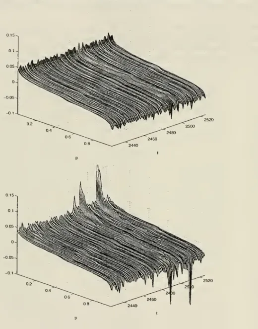
Surfaces

Figure 1 presents surfaces ofthe regression

VaR

functions plottedinthe time-probability level coordinates, (t,p). Recall that

p

is called the

proba-bility levelof

VaR, and

r

=

1

—

p

is the quantile index.

We

report

VaR

for all values of

_{p £}

[.01, .99].

The

conventional

VaR

reporting typically involves the probability levels of

p

=

.99

and

p

=

.95. Clearly, the

whole

VaR

surface

formed by

varying

p

in [.01,.99] represents a

more

complete

depiction of conditional risk.

Note

also that since

one

can beeither longor shortthe security,estimation of

VaR

inbothtailsofthereturndistribution

is ofinterest.

The

dynamics

depicted infigure 1

unambiguously

indicate certaindates

on which market

risk tends to be

much

higher

than

its usual level. This

by

itselfunderscores the

importance

of conditional modeling.

We

also stress

thatthe driving force

behind

the

dynamics

is the behavior of

X

t.

Model

Comparison

Figure 1 also

compares

the

dynamic

evolution of the linear

and

the

quadratic

VaR

surfaces. Notably, the quadratic

model

predicts higher risk

magnitudes than

thelinear model. Indeed, thefluctuations of thequadratic

VaR

surface are significantlylarger.

The

linear

model

thus predicts a

more

"smoothed

out"

VaR

surface.

Conditional Quantile

and

Quantile

Coefficient

Functions

The

nextseriesof figures presentsthestatistical aspectsoftheanalysis.

For brevity,

we

choseto present the results in agraphical form.20

Let ussetthedate at t

=

2500toanalyze the

VaR.

Figure2depicts the

estimated

VaR

2soo{p) for values of

p

inthe interval [.01, .99].21 This figure

also

shows

the

95%

confidenceintervals (c.i.) obtained

by

the following pro-cedures:22 (1)regular inference,based

on

theasymptotic

normal

approxima-tion (labeled as "asymptotic"), (2) resamplinginference,

by

the stationary

bootstrap, that is valid

under

regular

and

intermediate rank asymptotics,

and

(3)

and

(4):

subsampling

inference with different scaling schemes,

de-notedas

"Subsampling

I"

and "Subsampling

II," suitedfor

dependent

data,

and

valid

under

the

extreme

rank asymptotics.

Method

(1) is intended to

20

_We

have not presented here the formal statistical analysis ofthe quadratic

modelfor brevity.

Umantsev

and Chernozhukov(1999) offeradetailed analysis of

the quadratic model.

21

_We

computed

VaR(-) and coefficients forvalues ofplyingon agrid with cell size .01andinterpolatedinbetween.Thisisajustifiableinterpolation sinceVaR(-)

and coefficient processes are stochastically equicontinuous.

22

givethe confidenceintervalsthat are bestforthecentral values

p

£ [.1,-9],

method

(2) - forthe intermediate (near-extreme) values,

p

€ [.04,.96],

and

methods

(3)

and

(4)- for the

extreme

values

p

<E (0, .04]

and

[.96, l).24

As

can

be seen

from

figure2, thec.i.

by

methods

(2), (3),

and

(4) tend

tobe roughly 1.5, 2,

and

2.5timeswider

than

thestandardc.i.,respectively.

Hence

additional significant estimation uncertainty is present in the tails,

and

it is importantto properlyaccount forit.

Accounting

forit

means

that,

within the c.i. by

methods

(2)- (4), near-extreme

VaR

may

actually be as

much

as

two

times higher

than

thepointestimates suggest.

Figures 4-5 present the

same

analysis for the coefficient functions 6(-)

ofthe linearmodel.

The methods

and

the results

employed

are like those

we

havejust discussed.

We

will give

an

economic

meaning

tothe coefficient

shapes later.

Specification

Analysis

Figure 6 presents the pointwise values of

Wald

and

quasi-Score test

statistics for testingthe hypothesis:

—

Is theconventional (unconditionalhistorical)

VaR

model

statisticallynot

different

from

the conditional

VaR

model?

The

answer

isconclusive:the hypothesisis rejectedpointwise.

Note

that the'p-values'25 forthiscase areallsmaller

than

0.01.

That

is,the regression conditioning matters.Thiscanalso

be

seeninfigure4,

where

theconfidence

intervals ofslope coefficients are plotted

throughout

the interesting range

of

_p

-these confidenceintervalsexclude 0s.

Figure 6 (right) also depicts the specification test process (see earlier

section). Resultsofthe specification testingareclearly infavorofthe linear

model: the critical value (pointwise) for

10%

level is 6.25,

which

is

above

Based on Monte-Carlowith thesamplesizeof1000 andthe considerationsof

the previoussection.

In this application, for transparency and clarity, the subsampling methods

wereoperationalized by assumingthetails areexactly algebraic, sothat therate ofconvergenceor divergence is ar

=

T~*. £ wasestimated to beapproximately

.25 by the

method

described in the previous section. Hence

ar

=

T~'25 defined

ascalingfor thesubsamplingprocedure.

As

suggestedin Chernozhukov (1999a),

the centering constant was taken to be J3T{k/b).

The

subsample size b was set

to be1/10 ofthe whole sample T.

The

resulting confidenceintervals are labeled

"SubsamplingII." For comparison,rateaT

=

T

01wasalsoused,andtheresulting

confidence intervalswerelabeled as "SubsamplingI." 25

any

of the values depicted. Obviously, since the critical value for the test

statistic

sup

_{T6[001j 99}

j5c(t) should be

above

6.25, the linear

model

passes

thisstronger

Kolmogorov-type

test, too !

The

Determinants

of

Risk

We

now

provide

both

a statistical

and an economic

interpretation of

the coefficient functions #;(•). Let us fix time period t

=

2500

and suppose

for a

moment

that 9i(p)

>

for

some

i

>

0,p

6

(0,1).

As

VaR

t(p)

=

vt(p)

=

0o(p)

+

J2i9i(p)Xt,i, a positive coefficient in front of

X

t ,i implies

that higher values of

X

tji correspond to higher values of

VaR

t(p), given

that other elements of

X

t are

unchanged.

Stated differently, if_6i(p)

>

_0,

then increases (decreases) of

Xt

ti are associated with

upward

(downward)

shifts of

VaR

t{-) at pointp.

Note

that

VaR

t(-) is the "reversed" inverseof

the

cdioiy

t

\X

t, i.e.

F'^l

-

-\Xt) [Take figure3 (middle)

and

rotate it90°

clockwise togetthe conditional cdf.].

Thus

positive shocksin

X

t ,ishift the

cdf

F

_yt(-\Xt ) tothe right.

Similarly, if_9i(p) is negative, effects ofpositive

and

negative shocks in

the i th

information variable are reversed: positive shocks

move

VaR

t{p)

down

and

cdf of

yt\X

t totheleft

and

negative shocks

move

VaR

t(p)

up

and

cdf ofyt\Xt tothe right.

The

effectsdescribed

above

arelocal,inthe sense that theyaffect

VaR

t(•)

and

F

yt(-\Xt ) onlylocally,

around

points

p

and

F'^l

—p\X

t), respectively.

Transformations of these functions at other points caused

by

such shocks

depend on

the sign

and magnitude

of9i{p) at otherprobability levelsp.

Suppose

next that 9 is positive

and

decreasing in the right tail of

dis-tribution of yt\Xt (e.g. #i(-)

on

(0, .2), see figure 4).

A

positive shock in

Xi

will

now

shift the entire right tail ofcdf of

yt\X

t to the right,

and

the

effect will be greater for

extreme

points (those close to

p

=

0), at

which

9i(p) is higher.

The

effect

on

the density of_yt

\X

t is schematically depicted

in figure 7. Thus, this particular

shape

of6>i(-) implies that positiveshocks

ofthe corresponding informationvariable result in the righttail ofdensity ofyt\Xt being stretched further tothe right

(more

positiveskewnessin the

right tail).

A

similar

shape

is observed for the coefficient function

^(p)

for

almost allvalues ofp.

Thus, the shapesof0j(-)suchas#i(-)or^(-)infigure4 translate positive

shocksofthecorresponding informationvariables into the longer righttails

(favorable for holding long positions in Y).

On

the other hand, shapes of

9i(-) similarto those of6>3(-) in figure4 translate such shocks into shorter

Finally,

we

provide the

economic

interpretation of the slope coefficient

functions#i(-), #2(')i ^3(

-)> correspondingtothe laggedreturns

on

oil spot

price,

Xi,

equity index,

X2, and

priceofthe security inquestion,

X3.

—

9\(-) is significantly positive

and

decreasing in the right tail ofthe

dis-tribution ofyt\Xt (figures 4

and

5,

p

<

1/4). It is insignificantlypositive

in the middle part (for

p

€

(.25,.95))

and

then it is increasing in the

far left tail _(p

>

.96), although values Q\(p),

p

>

.96, are not as high

as those for

p

<

1/4. This suggests that the Spot price of Oil

and

the return

on

our stock are positively related, with the right tail of equity

return being

much

more

sensitive to Oil price shocks, than the left tail.

This effectcan be explainedby, for example,realoptionalityintrinsicto

the operation of the firm, or

by

a non-linear hedging policy (e.g., long

positions input options instead of

swaps

or futures,

whose

payoffis

lin-ear in the underlyingprice

movements).

The

overalleffect ofapositive

shockin thespot oilprice

X\

is presentedin figure 7.

—

#2(-)>

m

contrast, is significantly positive for all values of

p

with the

possibleexception ofthe far right tail ofyt\Xt, (p

€

(0,0.04)).

We

also

noticea

moderate

increaseintherighttail

and

asharpincreaseintheleft

tail(p closeto1).Thus,inadditiontothestrongpositiverelationbetween

the stock return

on

the individual stock

and

the

market

return (DJI)

(dictated

by

the fact that #2(-)

>

on

(0,1)) there is also additional

sensitivity ofthe lefttail ofthe securityreturnto the

market

movements

(steep increase

on

(.94, 1)),

which

is strongly consistent with the notion

of highly correlated equity returns in

market

drops. For high positive returns,incontrast,

market

returnhas a

much

weaker

effect (lowvalues

on

(0,0.04)).

The

effect of positive shock in the

market

return (X2) is

depicted in figure7.

—

#3(), in contrast, issignificantlynegative, exceptforvalues of

p

closeto

0. This

may

be clearly interpreted as a

"mean

reversion" effect in the

central part of the distribution.

However, X3,

the lagged return, does not

appear

tosignificantly shift thequantile function inthetails.

Thus

X3

is

more

importantforthe determination of intermediaterisks(values of

_p

in [.15,.85]).

The

effect ofa positive shock in

X3

is schematically portrayed in figure 7. Figures 4

and

7 also capture the

asymmetry

of

response tothenegative

and

positive return shocks- apositiveshockleads

to

mean

reversion

and

intermediate risk contraction, whereas a negative

Note

thattheestimates ofnear-extreme

VaR

should beinterpreted

care-fully, sincethe point estimates provided

by

regression quantiles are highly biased in the tails.

Some

correction can be achieved

by

using alternative

estimators that usethe regular variation properties oftailsin order to con-struct regression-likeestimates ofthe near-extreme

VaR

(seeprevious

sec-tion). For example, asdepicted inFigure 3, the regression extrapolation

es-timatorintroduces a significant correction, but within the confidence

bands

constructed

by

method

(4). Further conclusionsare stated insection 1.

Fig. 1 VaR,(p)for Linear (upper)and Qudratic (lower) Models (

VaR

t{p) ison

e2 a 3 a-a o 1-1 "0 a 1 in II

'M.

Fig. 4 Estimates and

95%

(Pointwise) Confidence Intervals for 6> (-),

24 VictorChernozhukov, Len

Umantsev

_r ' /'' /// '" v_l^ // / // ' OS _/ ' /// '/ -— /'' _/// ''/ c 1

—

/' /// '/ 3 V£S /,' I// ' '. " ' //I''/ c ^b J/ / / / ' / t-t '/' _{/ / /} '/' o ' /' / / / / CO ' / // / / ' nt >

''/////'

= S-. IU G

''/////'

' 1—4 ' ' /////' 1 Q> ' '

If

' U C ' 1111i i ' CD -n 1 (111i i ' <c ' 1111i ' i a ' 1i111 > o ' 1111j i

-U

_'III''

l *S ' ///// ' ' >n /// // ' ' ai

lllll

' -o ,////,/,', . , E : I

o J3 I a CM o in <B O Ph J3 tf 5e o

References

Ait-Sahalia,Y.,

and

A.

W.

Lo

(1998): "NonparametricRisk

Management

and

Implied Risk Aversion," preprint.

Bassett, G.,

AND

H.

Chen

(1999): "Quantile Style: Quantiles to Assess

Mu-tual

Fund

Investment Styles," a

Working

Paper,Presented at theInternational

Conference on

Economic

ApplicationsofQuantile Regression, Konstanz, 2000.

BASSETT, Jr.,

C,

and

R.

Koenker

(1978): "Asymptotictheoryofleastabsolute

error regression," J. Amer. Statist. Assoc, 73(363), 618-622.

BlERENS, H.,

AND

D. K.

GlNTHER

(1999): "IntegratedConditional

Moment

Test-ing ofQuantile Regression Models," a

Working

Paper,Presentedat the

Interna-tional Conferenceon Economic ApplicationsofQuantileRegression, Konstanz,

2000.

Campbell,

J., C.

MacKinlay,

AND

A.

Lo

(1997): Econometrics ofFinancial Markets.

MIT.

CHERNOZHUKOV,

V. (1999a): "Conditional Extremes and Near-Extremes,"

November, Ph.D. dissertation draft, Stanford.

(1999b): "Specification and Other Test Processes for Quantile

Regres-sion," August, a

Working

Paper, Stanford.

CHRISTOFFERSEN,

P. (1998): "Evaluating Interval Forecasts," International

Eco-nomic

Review, 39(4), 841-862.

CRNKOVIC,

C,

AND

J.

Drachman

(1996): "Quality Control," Risk, 9(9),

138-144.

DEKKERS,

A.L. M.,

AND

L.

DE

Haan

(1989):

"On

the estimationofthe extreme-valueindex and largequantile estimation," Ann. Statist., 17(4), 1795-1832.

Diebold, F. X., T. A.

Gunther,

and

A. S.

Tay

(1998): "Evaluating

Den-sityForecastswith ApplicationstoFinancial Risk Management," International

Economic

Review, 39(4), 863-883.

Engle,

R. F.,

AND

S.

Manganelli

(1999):

"CAViaR:

Conditional Autoregressive

ValueatRiskbyRegressionQuantiles,"

UCSD

Economics Deaprtment Working Paper99-20 , October.

FedReg

(1996): Risk-basedcapitalstandards: MarketRiskvol.61.FederalRegister.

FlTZENBERGER,

B. (1998): "The

moving

blocks bootstrapandrobustinferencefor

linear leastsquares andquantile regressions," J. Econometrics, 82(2), 235-287.

HEILER, S.,

AND

K.

ABBERGER

(1999): "ApplicationsofNonparametricQuantile RegressiontoFinancialData," a

Working

Paper, Presentedat theInternational

Conferenceon

Economic

ApplicationsofQuantile Regression, Konstanz, 2000.

Hogg,

R. V. (1975): "Estimates of Percentile Regression Lines Using Salary Data," J. Amer. Statist. Assoc, 70(349), 56-59.

KOENKER,

R.,

AND

G. S.

Bassett

(1978): "RegressionQuantiles," Econometrica,

46, 33-50.

KOENKER,

R.,

AND

J.

Machado

(1999): "Goodnessof Fit andRelatedInference

Processesfor Quantile Regression," preprint.

KOENKER,

R.,

AND

S.

PORTNOY

(1997): "The Gaussian Hare andthe Laplacian

Tortoise," Statistical Science, 12, 279-300.

KOENKER,

R.,

AND

S.

PORTNOY

(1999): "Regression Quantiles," preprint.

KOENKER,

R.,

and

Q.

Zhao

(1996): "Conditional quantile estimation and

infer-encefor

ARCH

models," Econometric Theory, 12(5), 793-813.

LOPEZ, J. A. (1998): "Regulatory Evaluation ofValue-at-Risk Models," Journal

of Risk, 1(2), 37-63.

POLITIS, D. N.,

and

J. P.

ROMANO

(1994): "Thestationarybootstrap," J. Amer.

Statist. Assoc, 89(428), 1303-1313.

PORTNOY,

S. (1991): "Asymptoticbehavior of regression quantilesin

nonstation-ary, dependentcases," J. Multivariate Anal., 38(1), 100-113.

RESNICK, S. I. (1987): Extreme values, regular variation, and point processes.

Taylor,

J. (1999): "A Quantile Regression Approach toEstimating the

Distri-bution ofMulti-Period Returns," J. Derivatives, Fall, 64-78.

Umantsev,

L.,

AND

V.

CHERNOZHUKOV

(1999): "Polynomial Regression Quantile

Modelingof Risk," September, a

Working

Paper, Stanford.

VAN

DER Vaart,

A.

W.,

AND

J. A.

Wellner

(1996):

Weak

convergence and

empirical processes. Springer- Verlag,

New

York.

Weiss, A. A. (1991): "EstimatingNonlinear

Dynamic

Models UsingLeast