The complexity of optimal mechanism design

The Complexity of Optimal Mechanism Design

by

Christos Tzamos

Submitted to the Department of Electrical Engineering and Computer

Science

in partial fulfillment of the requirements for the degree of

Master of Science in Computer Science and Engineering

at the

MASSACHUSETTS INSTITUTE OF TECHNOLOGY

June 2013

ARCHINES

IIXSSMCHiU5ETTINSTIfE OF TECHNOLOGY

JUL 0 8 2013

UBRARIES

@

Massachusetts Institute of Technology 2013. All rights reserved.

A u th or ...

Department of Electrical Engineering and Computer Science

May 22, 2013

C ertified by

....

.

.

,...

Constantinos Daskalakis

Associate Professor

Thesis Supervisor

Accepted by ...

...

K..o...o..d.z.ie.j.s.k.i

The Complexity of Optimal Mechanism Design

by

Christos Tzamos

Submitted to the Department of Electrical Engineering and Computer Science on May 22, 2013, in partial fulfillment of the

requirements for the degree of

Master of Science in Computer Science and Engineering

Abstract

Myerson's seminal work provides a computationally efficient revenue-optimal auction for sell-ing one item to multiple bidders. Generalizsell-ing this work to sellsell-ing multiple items at once has been a central question in economics and algorithmic game theory, but its complexity has remained poorly understood. We answer this question by showing that a revenue-optimal auction in multi-item settings cannot be found and implemented computationally efficiently, unless ZPP = P. This is true even for a single additive bidder whose values for the items are independently distributed on two rational numbers with rational probabilities. Our result is very general: we show that it is hard to compute any encoding of an optimal auction of any format (direct or indirect, truthful or non-truthful) that can be implemented in expected polynomial time. In particular, under well-believed complexity-theoretic as-sumptions, revenue-optimization in very simple multi-item settings can only be tractably approximated.

We note that our hardness result applies to randomized mechanisms in a very simple setting, and is not an artifact of introducing combinatorial structure to the problem by allowing correlation among item values, introducing combinatorial valuations, or requiring the mechanism to be deterministic (whose structure is readily combinatorial). Our proof is enabled by a flow interpretation of the solutions of an exponential-size linear program for revenue maximization with an additional supermodularity constraint.

Thesis Supervisor: Constantinos Daskalakis Title: Associate Professor

Acknowledgments

Foremost, I want to thank my advisor, Constantinos Daskalakis, for his constant help and guidance in the project and his encouragement throughout my life here at MIT. I want to thank my co-author and collaborator, Alan Deckelbaum for his contribution and for the hours we spent together working on the research problems in this thesis. I also want to thank the students of the TOC group for their helpful discussions and the fun time we had together.

Finally, I want to thank my parents, my brother, my girlfriend and all my friends, near or far, that are always close to me and support me through the difficult times in my life.

Contents

1 Introduction 1.1 O ur results . . . . 1.1.1 Pricing mechanisms . . . . 1.1.2 General Mechanisms . . . . 1.2 Contribution . . . . 1.3 Related Work . . . . 1.4 Further Results and Discussion . . . .

2 Hardness of Pricing Mechanisms

2.1 Prelim inaries . . . .

2.2 Hardness of Sum-of-Attributes Distributions . . . .

3 Overview of General Mechanisms

3.1 The Optimal Mechanism Design Problem . . . .

3.2 Structure of Optimal Mechanisms . . . .

3.3 Techniques . . . .

4 Computing General Multi-Item Mechanisms

4.1 Prelim inaries . . . . 4.1.1 Our Proof Plan . . . . 4.2 A Linear Programming Approach . . . .

4.2.1 Mechanism Design as a Linear Program . . . .

4.2.2 A Relaxed Linear Program . . . .

13 14 15 16 16 17 19 21 21 22 27 28 31 32 35 35 37 39 39 39

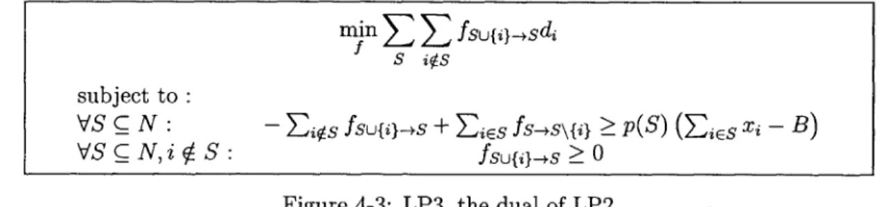
4.2.3 _{The Dual of the Relaxed Program as a Min-Cost Flow . . . . 42}

4.3 Characterizing the Linear Programming Solutions . . . . 43

4.3.1 The Canonical Solution to LP3 . . . . 43

4.3.2 _{From LP3 to LP2 Solutions . . . . 43}

4.3.3 _{From LP2 to LP1 Solutions . . . . 44}

4.3.4 Putting it All Together . . . . 46

5 Hardness of Multi-Item Mechanisms ₄₉ 5.1 _{Hardness of LEXRANK . . . . 49}

5.2 Hardness of Mechanism Design: Reduction from LEXRANK . . . . . . . . . . 51

6 Beyond Computationally Bounded Bidders 57 6.1 _{Budget-Additive Bidders . . . . 57}

6.2 _{Further Discussion: Powerful Bidders . . . . 58}

6.2.1 _{NP Power . . . . 58}

6.2.2 PSPACE and Beyond . . . . 59

List of Figures

4-1 LP1, the linear program for revenue maximization . . . . 39

4-2 LP2, the relaxed linear program . . . . 41

4-3 LP3, the dual of LP2 . . . . 42

List of Tables

Chapter 1

Introduction

Consider the problem facing a seller who is looking to sell items to bidders given distribu-tional information about their valuations, i.e. how much they value each subset of the items. This problem, called the optimal mechanism design problem, has been a central problem in economics for a few decades and has recently received considerable attention in computer science as well. The special case of a single item is well-understood: in his seminal paper [18], Myerson showed that the optimal single-item auction takes a simple form-when the values of the bidders for the item are independent. Moreover, if every bidder's value distribution is supported on rational numbers with rational probabilities, the optimal auction can be computed and implemented computationally efficiently-see e.g. [6]. On the other hand, the general (multi-item) problem has been open since Myerson's work and has remained poorly understood despite significant research effort devoted to its solution-see [16] and its references for work on this problem by economists.

More recently, the problem received considerable attention in computer science where algorithmic ideas have provided insights into its structure and computational complexity. Results have come in two flavors: approximations [8, 9, 4, 1, 15, 11], guaranteeing a constant fraction of the optimal revenue, and exact solutions [10, 6, 2, 7], guaranteeing full revenue extraction. These results provide comprehensive solutions to the problem, even under very general allocation constraints [7], but do not pin down its computational complexity. In par-ticular, all known exact mechanisms can be computed and implemented in time polynomial in the total number of valuations a bidder may have-i.e. the size of the support of each

bidder's valuation-distribution; so they are computationally efficient only when the valuation distributions are provided explicitly in the specification of the problem, by listing their sup-port together with the probability assigned to each valuation in the supsup-port. But this is not always the computationally meaningful way to describe the problem. The most trivial set-ting where this issue arises is that of a single additive bidder1 _{whose values for the items are}

independent of support two. In this case, the bidder may have one of 2" possible valuations, where n is the number of items, and explicitly describing her valuation-distribution would require Q(2") vectors and probabilities. However, a mechanism with complexity polynomial in Q(2") is clearly inefficient, and one would like to pay complexity polynomial in the dis-tribution's natural description complexity, i.e. the bits required to specify the disdis-tribution's n marginals over the items. Such efficient mechanisms have not been discovered, except in item-symmetric settings [10].

1.1

Our results

In this work, we study situations where we are given a more succinct description of the distribution of possible valuations. Previous work [5, 20, 11] has provided hardness results but only for special classes of mechanisms or complicated classes of valuations, failing to characterize the computational complexity of the optimal mechanism design problem. We achieve this by showing that optimal mechanism design is computationally intractable, even in the most trivial settings.

In particular, we consider the case where we only have one bidder who is additive over the items and her value for every item comes from an independent distribution of support two. As argued before, there is an exponential number of different valuation functions that the bidder may have but there exist implicit ways of describing them that are polynomial in the number of items, for example by writing down the marginal for each item.

Our work is divided in two parts. In the first part, we focus on deterministic mechanisms where we need to compute the price for one or multiple items while in the second we study

'An additive bidder is described by a value-vector (vi,... , Vn), where vi is her value for item i E [n), so

much more general mechanisms which are allowed to be randomized and may involve many phases of interaction between the seller and the bidders.

1.1.1

Pricing mechanisms

We consider first the problem of optimally pricing a single good for a single buyer whose val-uation is a sum of independent random variables. In our context, the probability distribution of the good's valuation has an exponentially sized support, but has a succinct description in terms of each component variable's distribution. The seller must choose a price to offer the good. The buyer will accept the offer (and pay the amount the seller asked for) if her valuation for the good is at least the price, and will reject the offer otherwise (giving the seller zero revenue). The seller's goal is to choose a price to maximize his expected revenue.

By Myerson [18), the best such pricing scheme is in fact the the optimal mechanism in this

setting.

This problem occurs fairly naturally. When selling a complex product (for example, a car), there are a number of attributes (color, fabric, size, etc) that a buyer may or may not value highly. The buyer's overall valuation of the car may be the sum of her valuation of the individual attributes. Assuming independence of the buyer's preferences for each attribute, her overall valuation of the car can be modeled as a sum of independent random variables.

We show that it is #P-hard to compute the optimal price. For our reduction, we consider a class of instances where we prove that there are only two candidate prices for extracting the optimal expected revenue. However, we show that distinguishing which of the two prices is better is equivalent to the counting version of the subset sum problem which is known to be #P-hard [22].

This hardness result can be directly translated to the multi-item setting. It corresponds to the simple case we described above, where there is one additive bidder and all items are independently distributed, under the restriction that items cannot be sold separately so a single price must be found for the bundle of all items.

1.1.2

General Mechanisms

The previous result for multi-item mechanisms only applies to mechanisms of a restricted format, selling all items for a single price. In fact, if this restriction is dropped, for all instances considered in our reduction, there exist different simple mechanisms that are easily computable and achieve higher revenue.

To show a much more general result, we consider general mechanisms under the very sim-ple setting we described above, making no assumptions about the format of the mechanism or how it is specified. We only require that the mechanism can be computed and executed in expected polynomial time. The main difficulty in proving hardness for this very relaxed problem is that, in contrast to the single-item case, the structure of the optimal mechanism is poorly understood. Even when there are only two items, the optimal mechanism may be very complicated and counter-intuitive and may require randomness to achieve high expected revenue. Therefore, a necessary step to analyze the problem is to identify a simple class of instances, for which we can understand the form of the solution. At the same time though, this class needs to be rich enough so that we are able to embed a hard problem and perform a hardness reduction.

In this work, we develop a framework that allows us to compute a class of instances whose solutions correspond to solutions to a well known combinatorial problem, the minimum-cost flow problem. This flow-interpretation enables us to understand the solution behavior. However, the flow instances we obtain are defined on exponential-size graphs with succinct description and therefore we cannot directly apply a flow algorithm to solve them efficiently. Using this class of instances, we obtain our main hardness result for Optimal Mechanism Design. We show that, unless ZPP = PO, we cannot efficiently compute a revenue-optimal

mechanism that can be executed in expected polynomial time.

1.2

Contribution

The contribution of our results is two-fold. First, we give a definitive proof that approxi-mation is necessary for revenue optimization beyond Myerson's single-item setting. Approx-imation has been heavily used in algorithmic work on the problem, but there has been no

justification for its use, at least in simple settings that don't induce combinatorial structure in the valuations of the bidders (sub-modular, OXS, etc.), or the allocation constraints of the setting. Second, our results represent advancement in our techniques for showing lower bounds for optimal mechanism design. Despite evidence that the structure of the optimal mechanism is complicated even in simple settings (see Section 3.3), previous work has not been able to harness this evidence to obtain computational hardness results. Our approach, using duality theory and flows to narrow into a family of instances for which this is possible, provides a new paradigm for proving hardness results in optimal mechanism design and, we expect, outside of algorithmic game theory. Again we note that complexity creeps in not because we assume correlations in the item values (which can easily introduce combinatorial dependencies among them), or because we restrict attention to deterministic mechanisms (whose structure is readily combinatorial), but because our approach reveals combinatorial structure in the optimal mechanism, which can be exploited for a reduction. See further discussion in Chapter 3.

1.3

Related Work

We have already provided background on optimal mechanism design in economics literature, as well as algorithmic solutions to the problem. We summarize the state of affairs in that exact, computationally efficient solutions are known for broad multi-item settings, as long as the bidder types are independent and their type-distributions are given explicitly. In particular, the runtime of such solutions is polynomial in the size of the support of each bidder's type-distribution, which may be exponential in the natural description complexity of the distribution, e.g., when the distribution is product over the items.

There has also been considerable effort towards computational lower bounds for the problem. Nevertheless, all known results are for either somewhat exotic families of valuation functions or distributions over valuations, or for unnatural correlated distributions.

In the first vein, Dobzinski et al. [11] show that optimal mechanism design for OXS bidders is NP-hard via a reduction from the CLIQUE problem. OXS valuations are described

Number of Items Simple Distributions [Simple Valuations I Unrestricted]

[DFK'11] many yes no yes

[Briest'08] many no yes no

[PP'11] one no yes no

Thm 1 one yes (implicit) yes yes

many yes yes no

Thm 2 many yes yes yes

Table 1.1: Summary of lower bounds for Optimal Mechanism Design. We provide the most general setting in which every result applies. For this purpose we compare the results based on different properties: Number of Items indicates whether the result is for single- or multi-item auctions. Simple Distributions indicates that the result does not depend on complicated correlated distributions to show hardness. Simple Valuations indicates that the result does not rely on artificial and highly combinatorial valuation functions to show hardness but instead uses simple valuation functions, e.g. additive or unit-demand. Unrestricted indicates that the result does not apply only to restricted classes of mechanisms (e.g. deterministic) but holds true for all possible mechanisms (even randomized). The more of these properties a lower-bound satisfies the more general it is.

implicitly via a graph, include additive, unit-demand2

and much broader classes of valuations, and are more amenable to lower bounds given the combinatorial nature of their definition.

(See further discussion in Chapter 6.)

Other related work shows lower bounds for mechanism design when the bidder valuations are simple but distributions are allowed to be correlated. Briest [5] shows inapproximability results for selling multiple items to a single unit-demand bidder via an item-pricing auction,3 when the bidder's values for the items are correlated according to some explicitly given distribution. More recently, Papadimitriou and Pierrakos [20] show APX-hardness results for the optimal, incentive compatible, deterministic auction when a single item is sold to multiple bidders, whose values for the item are correlated according to some explicitly given distribution. We note that for the settings of Briest [5] and Papadimitriou-Pierrakos [20] the restriction to deterministic mechanisms is crucial. The instances considered are polynomial-time solvable via linear programming when the determinism requirement is removed [11, 10].

2

A unit-demand bidder is described by a vector (Vi,... , Vn) of values, where n is the number of items. If the bidder receives item i, her value is vi, while if she receives a set of more than one item, her value for that set is her value for her favorite item in the set.

3

An item-pricing auction posts a price for each item, and lets the bidder buy whatever item s/he wants. It is clearly a deterministic auction as there is no randomness used by the auctioneer. A randomized auction for this setting could also be pricing lotteries over items.

Compared to these lower bounds, our goal is instead to prove intractability results for very simple valuations (namely additive) and distributions over them (namely the item values are independent and the distribution of each item is given explicitly) which have no combinatorial structure incorporated in their definition. Moreover, we aim to provide very general lower bounds without making any assumptions on the format of the mechanism or how it is specified. Table 1.1 summarizes the comparison between the different lower bounds. Furthermore, in a slightly different line of work, Hart and Nisan [14] introduce an alter-native notion for analyzing the complexity of auctions. They think of an auction as a large list of choices given to the buyers where each choice corresponds to a (possibly randomized) allocation of the items and a price. Given this representation, they study the menu-size complexity of auctions where mechanisms are ranked according to the number of choices they offer to the buyers.

We note that our results, translated to this setting, imply that menu-size complexity is not compatible with the notion of computational complexity that was considered above. Even when focusing on mechanisms with a menu of size one, it can be computationally hard to compute the optimal such mechanism. It is not difficult to verify that the optimal mechanism of menu-size one is deterministic and offers the bundle of all the items for the optimal bundle price [14]. However, as we show in Theorem 1, computing the optimal such price is #P-hard.

1.4

Further Results and Discussion

In addition to our main results, we show that, beyond additive valuations, computational intractability arises for very simple settings with submodular valuations, namely even for a single, budget-additive,4 quasi-linear bidder whose values for the items are perfectly known, but there is uncertainty about her budget. This is presented as Theorem 3 in Section 6.1.

Interestingly, the hard instances constructed in the proof of Theorem 3 have trivial in-direct mechanism descriptions, but require NP power for the bidder to determine what to

4

A budget-additive bidder is described by a value-vector (vi, ... , v), where vi is her value for item i E [n],

buy. We show that this phenomenon is quite general, discussing how easily implementable, optimal, indirect mechanisms may be trivial to compute, if the bidders are assumed suffi-ciently powerful computationally. This is discussed in Section 6.2, and further justifies the assumptions about the computational abilities of the bidders made in our framework (in Section 3.1) for studying the complexity of optimal mechanism design.

Chapter 2

Hardness of Pricing Mechanisms

2.1

Preliminaries

To illustrate the problem that arises when considering implicitly defined distributions, we first consider the problem of optimally pricing a single good for a single buyer whose valuation is a sum of independent random variables with support 2. In our context, the probability distribution of the good's valuation has an exponentially sized support, but has a succinct description in terms of each component variable's distribution. The seller must choose a price P to offer the good. The buyer will accept the offer (and pay P) if her valuation is at least P, and will reject the offer (giving the seller zero revenue) if her valuation is strictly less than P. The seller's goal is to choose P to maximize his expected revenue. By Myerson [18], the best such pricing scheme is in fact the the optimal mechanism in this setting.

This problem occurs fairly naturally. When selling a complex product (for example, a car), there are a number of attributes (color, fabric, size, etc) that a buyer may or may not value highly. The buyer's overall valuation of the car may be the sum of her valuations of the individual attributes. Assuming independence of the buyer's preferences for each attribute, her overall valuation of the car can be modeled as a sum of independent random variables.

Definition 1 (Sum-of-Attributes Pricing). We define the Sum-of-Attributes Pricing problem as follows: Given n pairs of nonnegative integers (u1, v1), (u2, v2),- -, (un, vn) and

Pr[Z'l Xi > P*], where the Xi are independent random variables taking value ui with probability pi and vi with probability 1 - pi.

Equivalently, we can view the Sum-of-Attributes Pricing problem in the multi-item setting as a Grand Bundle Pricing problem. In this setting, there is a seller with n items and a buyer whose values for the items X1, ... , Xn are independent random variables drawn from known distributions. We seek the optimal price to sell the "grand bundle", i.e. the collection of all n goods, such that the seller maximizes his expected revenue. We assume that the buyer is additive, meaning that her value for the grand bundle is simply the sum

E

Xi of her values for the individual items. As discussed in [17], selling only the grand bundle is optimal in several natural contexts. Furthermore, bundling oftentimes has a revenue guarantee close to the optimal mechanism [13]. The problem of optimally pricing the grand bundle is furthermore interesting in its own right [12].

2.2

Hardness of Sum-of-Attributes Distributions

The next theorem shows that the task of determining the optimal price P can be hard, even in this simple setting.

Theorem 1. The Sum-of-Attributes Pricing problem and the Grand Bundle Pricing problem are #P-hard.

Proof. We will show how to use oracle access to solutions of the GBP problem to solve the counting analog of the subset sum problem, which is #P-complete. 1

The idea of our proof is to design an instance of the GBP problem for which the optimal price is one of two possibilities. A single parameter (in this case, the probability Pn+1 for the last good) determines which of these two options is optimal. By repeatedly using a GBP oracle and varying the value of Pn+1, we can determine the exact threshold value of Pn+1, which provides sufficient information to deduce the answer to the #-subset sum problem.

Given an input {ao, a1,... , an_1} and a target T <

E

ai of positive integers to the

#-subset sum problem, our goal is to determine the number of #-subsets of the ai's which sum 'Indeed, the reduction from SAT to SUBSET-SUM as presented in [22] is parsimonious.

to at least T.

We create an input to GBP containing n

+

1 items, where each of the first n items have

ui = ai and vi = 0. The value of item n + 1 has un+1 = T

+

1 and v"+1 =

1-For the first n items, we fix

A 1

2"n(n+1+E"

ai)2-Observe that each of these items has the same pi value. The probability of all n of these items being 0 is:

n a.)2) 1

2nn(n + 1 +

E>1-

2n(n + 1 + E"1 a)2

which is very close to 1.

We denote by p the (currently undetermined) probability pn+1 for the last item having value T

+

1.

Consider pricing the grand bundle at value B. We have the following claims:

1. If B = 1, the expected revenue is 1.

2. If 1 < B < T

+

1, then the expected revenue is at most

B p+ + ₁ P n

2"(n + 1 + E"= ai)2

3. If B = T

+

1, then the expected revenue is at least p(T + 1).

4. If T

+

1 < B < T ± 1

+

" aj, then the expected revenue is at most

n1 _{1 +}

_E"

_ai

T + 1 +

ai

< 1 a < 1.

2n(n

+1 + E"

ai)2J 2n'(n + 1 +

ai2

5. If B>T±+1+ " aj, then the expected revenue is 0.

The fourth and fifth cases are never optimal, since they are both dominated by setting B = 1. We claim that the second case is likewise never optimal. Suppose for the sake of

were optimal. Then we would have the following two constraints:

* B

(P

+

2n(n±1±Z 1ai)2 >

* B

(p+

2"(n+1+n ja)2) > (T + 1)p. Let

2n(n +1+ ai)2

We will now show that no value of p exists for which both of the above constraints are simultaneously satisfied. From the first constraint, we deduce p + E(1 - p) > 1/B and thus

1/B - e 1/T - E

p-c;> >- > 1/T -c.

Since T <

E

aj, we know that

1 1 1 1 1

1/T - E > 1 - > >

-Ea a 2"(n=+1+ a)2 _~E

_a

_2nEaj

_{- 2Eai'}

Therefore, the first constraint implies that p > 2

-From the second constraint, we deduce B(p + e(1 - p)) > (T + 1)p and thus

Be - T + 1 - B + BE Since B < T, we know that T + 1 - B + BE > 1. Therefore,

p < BE <Te <EajE= _{2n(n + 1 +}

_En

* , _ai)2 <

₂

_E

.

a;

Both constraints on p cannot be satisfied simultaneously. In summary, we have shown the following:

For any p, the optimal grand bundle price is either 1 or T + 1.

We note the monotonicity property that if, for some p, the optimal bundle price were T

+

1, then the optimal price would be T

+

1 for any p' > p.2 Therefore, for any T, there

2

This follows from the fact that the expected revenue from selling the bundle at T + 1 will only increase as p increases.

exists a unique p' for which the expected revenue of selling the bundle at price T + 1 is exactly the same as the expected revenue of selling the bundle at price 1.

We denote by V the total value of the first n items. Suppose that we have found a p* such that the expected revenue of selling the grand bundle at T + 1 is exactly 1. (We notice that such a p* must satisfy p*(T

+

1) < 1.) Then

1 = (T + 1) (p* + (1 - p*)P[V > T])

and thus 1- (T + 1)p* P >p* Furthermore, P* 1/(T + 1) - P[Vn >: T] 1 - P[V > T]

Therefore, if we could solve for p*, it would be simple arithmetic to compute P[V ;> TI.

We notice that _n

P[Vn > T]

=

p1

-p1)n-k -

S(k,T)

k=0

where S(k, T) is the number of subsets of the ai which sum to at least T. By our choice of pi being sufficiently small, we know furthermore that (1 - pi)/pi > 2"n, and therefore

p1- pi)i > 2"p--1(1 - pi)n-i- for all i. This means, in particular, that we can greedily

compute S(k, T) for each k by starting with k = 0 and setting S(k, T) to be as large as

possible consistent with the already assigned S values and the computed value of P[V, > T]. We exactly solve for p* using binary search: In each step of the search, we use an oracle for the GBP problem to determine if the optimal grand bundle price is 1 or T +1. Since there are only 2" possible values of P[V > T] (and specifying each requires only a polynomial number of bits3), we would need at most n calls to the GBP oracle to exactly determine p*.

E

This result demonstrates the difficulty of designing multi-dimensional distributions when the joint distribution of the items is not expilicitely given in the input. However, it does not

completely pin down the complexity of multi-dimensional mechanism design, since one could come up with a better mechanism, not restricted to selling all items together, that is easier to compute and achieves higher revenue. In fact, for all instances considered in the reduction, the simple mechanism that sells each item independently achieves higher revenue than selling the grand bundle. In the next few chapters, we tackle this problem and provide much more general complexity results making no assumptions about the format of the mechanism or how it is specified.

Chapter 3

Overview of General Mechanisms

The results of the previous chapter apply to multi-item mechanisms of a restricted format, selling all items for a single price. If this restriction is dropped it is not clear whether there is an efficient mechanism that computes and runs the optimal auction. Our goal in the following two chapters, is to investigate the behavior of general mechanisms and provide lower bounds on their complexity. We characterize the optimal mechanism for a sufficiently large class of input instances and then use those to reduce a computationally hard problem to the problem of optimal mechanism design. Our main result is the following:

Theorem 2. There is no expected polynomial-time solution to the optimal mechanism design problem (formal definition in Section 3.1) unless ZPP D P#P.

Moreover, it is #P-hard to determine whether every optimal mechanism assigns a specific item to a specific type of bidder with probability 0 or with probability 1 (at the Bayesian Nash equilibrium of the mechanism), given the promise that one of these two cases holds simultaneously for all optimal mechanisms.

The above are true even in the case of selling multiple items to a single additive, quasi-linear' bidder, whose values for the items are independently distributed on two rational

num-bers with rational probabilities.

'A bidder is quasi-linear if her utility for purchasing a subset S of the items at price ps is vs - Ps, where vs is her value for S.

3.1

The Optimal Mechanism Design Problem

To explain our result, we describe the Optimal Mechanism Design (OMD) problem more formally. As we are aiming for a broad lower bound we take the most general approach on the definition of the problem placing no constraints on the form of the sought after mechanism, or how this mechanism is meant to be described. Hence, our lower bounds apply to computing direct revelation mechanisms as well as any conceivable type of mechanism.

INPUT: This consists of the names of the items and the bidders, the allocation constraints of the setting (specifying, e.g., that an item may be allocated to at most one bidder, etc.), and a probability distribution on the valuations, or types, of the bidders. The type of a bidder incorporates information about how much she values every subset of the items, as well as what utility she derives for receiving a subset at a particular price. For example, the type of an additive quasi-linear bidder can be encapsulated in a vector of values (one value per item). We won't make any assumptions about how the allocation constraints are specified. In general, these could either be hard-wired to a family of instances of the OMD problem, or provided as part of the input in a computationally meaningful way. For the purposes of our intractability results, the allocation constraints will be trivial, enforcing that we can only allocate at most one copy of each item, and we restrict our attention to instances with precisely these allocation constraints. As far as the type distribution is concerned, we restrict our attention to additive quasi-linear bidders with independent values for the items. So, for our purposes, the type distribution of a bidder is specified by specifying its marginal on each item. We assume that each marginal is given explicitly, as a list of the possible values for the item as well as the probabilities assigned to each value.2

DESIRED OUTPUT: _{The goal is to compute a (possibly randomized) auction that optimizes,}

over all possible auctions, the expected revenue of the auctioneer, i.e. the expected sum of prices paid by the bidders at the Bayes Nash equilibrium of the auction,3 where the

2

There are of course other ways to describe these marginals. For example, we may only have sample access to them, or we may be given a circuit that takes as input a value and outputs the probability assigned to that value. As our goal is to prove lower bounds, the assumption that the marginals are provided explicitly in the input only makes the lower bounds stronger.

3

Informally Bayesian Nash equilibrium is the extension of Nash equilibrium to incomplete-information games, i.e. games where the utilities of players are sampled from a probability distribution. We won't provide a formal definition as it is quite involved and is actually not required for our lower bounds, which

expectation is taken with respect to the bidders' types, the randomness in their strategies (if any) at the Bayes Nash equilibrium, as well as any internal randomness that the auction uses.

We note that there is a large universe of possible auctions with widely varying formats, e.g. sealed envelope auctions, dynamic auctions, all-pay auctions, etc. And there could be different auctions with optimal expected revenue. As our goal is to prove robust intractability results for OMD, we take a general approach imposing no restrictions on the format of the auction, and no restrictions on the way the auction is encoded. The encoding should specify in a computationally meaningful way what actions are available to the bidders, how the items are allocated depending on the actions taken by the bidders, and what prices are charged to them, where both allocation and prices could be outputs of a randomized function of the bidders' actions. In particular, a computationally efficient solution to OMD induces the following:

AUCTION COMPUTATION&SIMULATION: A computationally efficient solution to a

family I of OMD problems induces a pair of algorithms C and S satisfying the following:

1. [auction computation] C : I -+ S is an expected polynomial-time algorithm

map-ping instances I E I of the OMD problem to auction encodings C(I) E E; e.g. C(I) may be "second price auction", or "English auction with reserve price $5", etc.

2. [auction simulation] S is an expected polynomial-time algorithm mapping in-stances I E I of the OMD problem, encodings C(I) of the optimal auction for I, and realized types ti,.. . , tm for the bidders, to a sample from the (possibly ran-domized) allocation and price rule of the auction encoded by C(I), at the Bayes Nash equilibrium of the auction when the types of the bidders are ti, ... , tm.

Clearly, Property 1 holds because computing the optimal auction encoding C(I) for an

in-focus on the single-bidder case.

For the purposes of the problem definition though, we note that, if an auction has multiple Bayesian Nash equilibria, its revenue is not well-defined as it may depend on what Bayesian Nash equilibrium the bidders end up playing. So we would like to avoid such auctions given the uncertainty about their revenue. Again this complication won't be relevant for our results as all auctions we construct in our hardness proofs will have a unique Bayes Nash equilibrium.

stance I is assumed to be efficient. But why does there exist a simulator S as in Property 2? Well, when the auction C(I) is executed, then somebody (either the auctioneer, or the bid-ders, or both) need to do some computation: the bidders need to decide how to play the auction (i.e. what actions from among the available ones to use), and then the auctioneer needs to allocate the items and charge the bidders. In the special case of a direct Bayesian Incentive Compatible mechanism,4 the bidders need not do any computation, as it is a Bayes Nash equilibrium strategy for each of them to truthfully report their type to the auctioneer. In this case, all the computation must be done by the auctioneer who needs to sample from the (possibly randomized) allocation and price rule of the mechanism given the bidders' reported types. In general (possibly non-direct, or multi-stage) mechanisms, both bidders and auctioneer may need to do some computation: the bidders need to compute their Bayes Nash equilibrium strategies given their types, and the auctioneer needs to sample from the (possibly random) allocation and price rule of the mechanism given the bidders' strategies. These computations must all be computationally efficient, as otherwise the execution of the auction C(I) would not be computationally efficient. Hence an efficient solution must induce an efficient simulator S. Notice, in particular, that S requires that the combined computa-tion performed by bidders and auccomputa-tioneer be computacomputa-tionally efficient. This is important as placing no computational restrictions on the bidder side easily leads to spurious "efficient" solutions to OMD, as discussed in Section 6.2.

In view of the above discussion, Theorem 2 establishes that, even in very simple special cases of the OMD problem, there does not exist a pair (C, S) of efficient auction computa-tion and simulacomputa-tion algorithms, i.e. the optimal auccomputa-tion cannot be found computacomputa-tionally efficiently, or cannot be executed efficiently, or both. We note that our hardness result is subject to the assumption ZPP 2 P#P (rather than P Z P#P) solely because we prove lower bounds for randomized mechanisms.

Remark 1 (Hardness of BIC Mechanisms). A lot of research on optimal mechanism design has focused on finding optimal Bayesian Incentive Compatible (BIC) mechanisms, as focusing on such mechanisms costs nothing in revenue due to the direct revelation principle (see [19]

4_{A mechanism is direct if the only available actions to a bidder is to report a type in the support of her}

type-distribution. A direct mechanism is Bayesian Incentive Compatible if it is a Bayes Nash equilibrium for every bidder to truthfully report her type to the auctioneer.

and Section

4.1).

As an immediate corollary of Theorem 2 we obtain that it is #P-hard to compute the (possibly randomized) allocation and price rule of the optimal BIC mechanism (Corollary 1 in Section

4.

1). However, Theorem 2 is much broader, in two respects: a. in the

definition of the OMD problem we impose no constraints on what type of auction should be found; b. we don't require an explicit computation of the (possibly randomized) allocation and price rule of the mechanism, but allow an expected polynomial-time algorithm that samples from the allocation and price rule.

3.2

Structure of Optimal Mechanisms

There are serious obstacles in establishing intractability results for optimal mechanism de-sign, the main one being that the structure of optimal mechanisms is poorly understood even in very simple settings. To prove Theorem 2, we need to find a family of mechanism design instances whose optimal solutions are sufficiently complex to enable reductions from some #P-hard problem, while at the same time are sufficiently restricted so that solutions to the #P-hard problem can actually be extracted from the structure of the optimal mechanism. However, there is no apparent structure in the optimal mechanism even in the simple case of a single additive bidder.

To gain some intuition, it is worth pointing out that the optimal mechanism for selling multiple items to an additive bidder is not necessarily comprised of the optimal mechanisms for selling each item separately. Here is an example from Hart and Nisan [13]. Suppose that there are two items and the bidder's value for each is either 1 or 2 with probability

j,

independently of the other item. In this case, the maximum expected revenue from selling the items separately is 2, achieved e.g. by posting a price of 1 on each item. However, offering instead the bundle of both items at a price of 3 achieves a revenue of 3 ₄ - _4*

On the other hand, bundling the items together is not always better than selling them separately. If there are two items with values 0 or 1 with probability i, independently from each other, then selling the bundle of the two items achieves revenue at most

j,

but selling the items separately yields revenue of 1, which is optimal.

selling the grand bundle of all the items, or selling each item separately, even when the item values are i.i.d. In fact, the optimal mechanism might not even be deterministic: we may need to offer for sale not only sets of items, but also lotteries over sets of items. Here is an example. Suppose that there are two items, one of which is distributed uniformly in {1, 2} and the other uniformly in {1, 3}, and suppose that the items are independent. In this case, the optimal mechanism offers the bundle of the two items at price 4, and it also offers at price 2.5 a lottery that with probability

j

gives both the items and with probability

}

just

the first item.5

3.3

Techniques

Given that optimal mechanisms have no apparent structure, even in the simple case of an additive bidder with independent values for the items, the main challenge in proving our hardness result is pinning down a family of sufficiently interesting instances of the problem for which we can still characterize the form of the optimal mechanism. To do this we follow a principled approach starting with a folklore, albeit exponentially large, linear program for revenue optimization, constructing a relaxation of this LP, and showing that, in a suitable class of instances, the solution of the relaxed LP is also a solution to the original LP, which has rich enough structure to embed a #P-hard problem. In more detail, our approach is the following:

" In Section 4.2.1 we present LP1, the folklore, albeit exponentially large, linear program

for computing a revenue optimal auction.

" In Section 4.2.2 we relax the constraints of LP1 to construct a new, still exponentially

large, linear program LP2. The solutions of the relaxed LP need not provide solu-tions to the original mechanism design problem. We prove however that an optimal LP2 solution is indeed an optimal LP1 solution if it happens to be monotone and supermodular.

* In Section 4.2.3 we take LP3, the dual program to LP2. We interpret its solutions as solutions to a minimum-cost flow problem on a lattice.

5

" In Section 4.3.1 we characterize a canonical solution to a specific subclass of LP3 instances. This solution requires ordering of the subset sums of an appropriate set of integers.

* In Section 4.3.2 we use duality to convert a canonical LP3 solution to a unique LP2 solution. We are therefore able to characterize the unique solution for a variety of LP2 instances.

" In Section 4.3.3 we show that the LP2 solutions obtained above are also feasible and

optimal for the corresponding LP1 instance. Thus, we gain the ability to characterize unique optimal solutions of a class of LP1 instances.

" Finally, using the previous characterization, in Chapter 5 we show how to encode a

Chapter 4

Computing General Multi-Item

Mechanisms

4.1

Preliminaries

We restrict our attention to instances of the mechanism design problem where a seller wishes to sell a set N =

{1,

2, ..., n} of items to a single additive quasi-linear bidder whose values

for the items are independent of support 2. In particular, the bidder values item i at aj, with probability 1 -pi, and at ai + di, with probability pi, independently of the other items, where aj, di, and pi are positive rational numbers. If she values i at aj, we say that her value for i is "low" and, if she values it at ai + di, we say that her value is "high." The specification of the instance comprises the numbers {ai, di, pi} 1.

A mechanism M for an instance I as above specifies a set A of actions available to the

bidder together with a rule mapping each action a E A to a (possibly randomized) allocation

A, E {O, 1}", specifying which items the bidder gets, and a (possibly randomized) price -o E R that the bidder pays, where A, and -r could be correlated. Facing this mechanism, a bidder whose values for the items are instantiated to some vector V E Xi{ai, ai + di} chooses any action in arg maxEA{- E(Aa) - E(ra)} or any distribution on these actions, as long as the maximum is non-negative, since iI. E(A0 ) - E(r) is the expected utility of the bidder for

choosing action a.' In particular, any such choice is a Bayesian Nash equilibrium behavior

for the bidder, in the degenerate case of a single bidder that we consider.2 _{If for all vectors V} there is a unique optimal action ag E A in the above optimization problem, then mechanism

M induces a mapping from valuations f E x i{ai, ai+di} to (possibly randomized) allocation and price pairs (Aa, r ,). If there are i's with non-unique maximizers, then we break ties in favor of the action with the highest E(T) and, if there are still ties, lexicographically beyond that.3

In Section 3.1 we explained in detail what it means to solve an instance I = {ai, di, pi}'

computationally efficiently. In short, the solution needs to encode the action set A as well as the mapping from actions a E A to (Aa, Ta), _{in a way that given an instantiated type}

i E _{xi{ai, ai + di} we can computationally efficiently sample from Aa, and from Tar,.}

It is convenient for our arguments to first study direct mechanisms, where the action set available to the bidder coincides with her type space xi{ai, ai + di}. In this case, we can equivalently think of the actions available to the bidder as declaring any subset S C N, where the correspondence between subsets and value vectors is given by if(S) = EiEN aiei +

EiS

die, where ei is the unit vector in dimension i; i.e. S represents the items whose values

are high. For all actions S C N, the mechanism induces a vector q'(S) E [0, 1]n of probabilities that the bidder receives each item and an expected price r(S) E R that the bidder pays. The expected utility of a bidder of type

V(S)

for choosing action

S'

is given by V(S) - (S') - T(S').

We denote by u(S) = if(S) - i(S) - r(S) her expected utility for reporting her true type. The

following are important properties of direct mechanisms.

Definition 2. A direct mechanism for the family of single-bidder instances we consider in

this thesis is Bayesian Incentive Compatible (BIC) if the bidder cannot benefit by misreporting the set of items he values highly. Formally:

VS, T C N : (S) -i(S) - r(S) ;> (S) -q(T)- T(T).

include in A a special action "stay home" that results in the bidder getting nothing and paying nothing. If all other actions give negative utility the bidder could just use this special action.

2

As mentioned earlier, we opt not to define Bayesian Nash equilibrium for multi-bidder mechanisms as this definition is involved and irrelevant for our purposes.

3

We can enforce this tie-breaking with an arbitrarily small hit on revenue as follows: For all a, we decrease the (possibly random price) -r output by M by a well-chosen amount-think of it as a rebate-which gets larger as E(r) gets larger. We can choose these rebates to be sufficiently small so that they only serve the purpose of tie-breaking. These rebates won't affect our lower bounds.

Or, equivalently:

VS, T C N: u(S) > u(T) + (V(S)

-

U(T)) -e(T).

Definition 3. The mechanism is individually rational (IR) if u(S) 0, for all S C N.

We note that an immediate consequence of our proof of Theorem 2 is the following.

Corollary 1. Given an instance I = {ai, di, pi } of the optimal mechanism design problem

(i.e. the same setting as Theorem 2), it is #P-hard to compute circuits (or any other implicit

but efficient to evaluate description of) q : x{ai, ai+diJ -+ [0, 1]" and T : xi{ai, ai+di -+ R inducing a revenue-optimal, BIC, IR mechanism.

Note that, for a meaningful lower bound, we cannot ask for q(S), r(S) for all S, as there are too many S's-namely 2". Instead we need to ask for some implicit but computationally meaningful description of them, such as in the form of circuits, which can be evaluated on an input S in time polynomial in their size and the number of bits required to describe S-if we don't require that q and r can be evaluated efficiently on any given S we would allow for trivial solutions such as "I is itself an implicit description of the optimal q and r for I." We conclude with the following remark.

Remark 2. For the single-bidder instances we consider in this thesis, a direct mechanism that is Bayesian Incentive Compatible is also Incentive Compatible and vice versa.4 As

all our hardness results are for single-bidder instances, they simultaneously show the in-tractability of computing optimal Bayesian Incentive Compatible as well as optimal Incentive

Compatible mechanisms.

4.1.1

Our Proof Plan

To prove Theorem 2 we narrow into a family of single-bidder instances (of the form de-fined in the beginning of this section) for which there is a unique optimal BIC, IR, direct

4_{For the reader who is not familiar with these concepts here is a brief explanation. A direct multi-bidder}

mechanism is Incentive Compatible if, for all bidders i and all ti, it is optimal for bidder i to truthfully report ti no matter what the other bidders report. It is a stronger notion than Bayesian Incentive Compatibility which requires that, for all bidders i and all ti, it is optimal for bidder i to truthfully report ti, if the other bidders also truthfully report their types in expectation with respect to their realized types. I.e. the latter concept requires that it is Bayesian Nash equilibrium for every bidder to truthfully report their type, while the former concept requires that it is a Dominant Strategy equilibrium for every bidder to truthfully report their type. Clearly, the two concepts collapse if there is just one bidder.

mechanism, and this mechanism satisfies the following: for a special item

i*

and a special type S*, qj. (S*) E {0, 1} but it is #P-hard to decide whether q. (S*) = 0. Our approach for

narrowing into this family of instances was outlined in Section 3.3 and is provided in detail in Sections 4.2 through 5. These sections establish two hardness results: First, they show Corollary 1 that it is #P-hard to compute circuits for q and r, as if we could compute such circuits in polynomial time then we would also be able to answer whether qi.(S*) = 0 in polynomial time. Second, they establish Theorem 2 restricted to BIC mechanisms. Indeed, if there were expected polynomial-time algorithms C, S (see Section 3.1), then we would plug in type S* and get one sample from the allocation rule for that type. Notice that this sample will allocate item

i'*

if and only if qi.(S*) = 1, which is #P-hard to decide. Details

are provided in Chapter 5.

Finally, it is straightforward to translate this hardness result to general mechanisms by making the following observation, called the "Revelation Principle" [19]:

9 Any (possibly non-direct) mechanism M has an equivalent BIC, IR, direct mechanism

M' so that the two mechanisms induce the exact same mapping from types V to (possibly randomized) allocation and price pairs. Indeed, as explained above, given the (possibly randomized) allocation rule A and price rule r of M we can define the mapping V '-* (Aa,, r,). This mapping is in fact itself a BIC, JR direct mechanism

M'.

Clearly, M and M' have the same expected revenue.

As mentioned above, the hard instances we narrow into in our proof satisfy that their optimal BIC, IR direct mechanism is unique and it is a #P-hard problem to tell whether qj* (S*) = 0 or 1 for a special item i* and a special type S*. The above observation implies that, for any instance in our family, any (possibly non-direct) optimal mechanism M for this instance needs to induce an optimal direct mechanism. Since the latter is unique, M needs to give the same (possibly randomized) allocation to type S* that the unique direct mechanism does. As argued above, getting one sample from this allocation allows us to decide whether

qj* (S*) = 1, a #P-hard problem. As any efficient solution to our family of OMD instances

would allow us to get samples from the allocation rule of an optimal mechanism in expected polynomial-time, we would be able to solve a #P-hard problem in expected polynomial-time. This establishes Theorem 2 (for unrestricted mechanisms).

4.2

A Linear Programming Approach

Our goal in Sections 4.2 through 5 is showing that it is computationally hard to compute a BIC, IR direct mechanism that maximizes the seller's expected revenue, even in the single-bidder setting introduced in Section 4.1. In this section, we define three exponential-size linear programs which are useful for zooming into a family of hard instances that are also amenable to analysis. Our LPs are defined using the notation introduced in Section 4.1.

4.2.1

Mechanism Design as a Linear Program

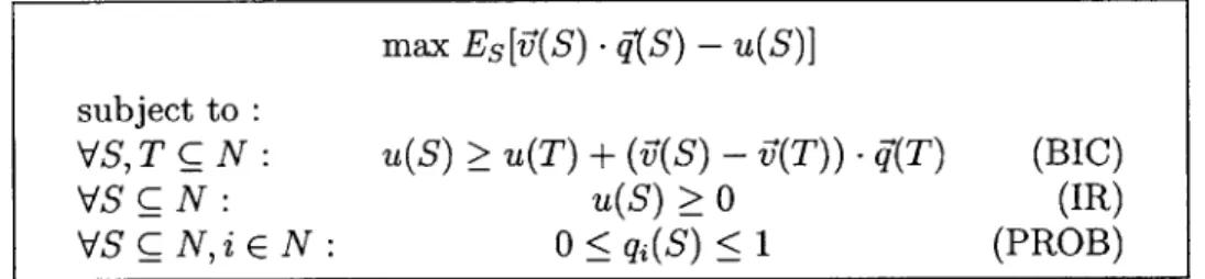
The optimal BIC and IR mechanism for the family of single-bidder instances introduced in Section 4.1 can be found by solving the following linear program, which we call LP1:

max Es[V(S) - f(S) - u(S)]

subject to :

VS, T C N: u(S) > u(T) + (V(S) - V'(T)) - q(T) (BIC)

VS C N: u(S) 2 0 (IR)

VS C NiE N: 0 < ql(S) < 1 (PROB)

Figure 4-1: LP1, the linear program for revenue maximization

Notice that the expression V(S) -i(S) - u(S) in the objective function equals the price r(S) that the bidder of type S pays when reporting S to the mechanism. The expectation is taken over all S C N, where the probability of set S is given by p(S) = ILES Pi - HS(1 - Pi). We notice that this program has exponential size (variables and constraints).

4.2.2

A Relaxed Linear Program

We now remove constraints from LP1 and perform further simplifications, making the pro-gram easier to analyze. Later on we identify a subclass of instances where optimal solutions to the relaxed program induce optimal solutions to the original program (see Lemma 3).

As a first step, we relax LP1 by considering only BIC constraints that correspond to neighboring types (types that differ in one element). We also drop the constraint that the probabilities qi(S) are non-negative:

max

Es[fi(S) -q(S)

-

u(S)]

subject to :

VS C N, i

V

S:

u(S

U

{i})

u(S) + diqi(S)

(BIC1)

VS C N,

i

V S: u(S) u(S U {i}) - diqi(S U

{i})

(BIC2)

VS C

N:

u(S) >

0

(IR)

VS

C

N, i E N: qi(S)

< 1

(PROB')

Since the coefficient of every qi(S) in the objective is strictly positive, no qi(S) can be increased in any optimal solution without violating a constraint. We therefore conclude the following about qi(S):

" If i E S, then qi(S) is only upper-bounded by constraint PROB', and thus qi(S) = 1

in every optimal solution.

" If i V S, then qi(S) = min{1, u(su{l})-u(s)} _{from (BIC1) and (PROB'). Furthermore,}

from (BIC2) we have u(sufi})-u(s) < qi(S U{i = 1, and thus q (S) - u(sufi})-u(s)

So the program becomes (after setting q(S) = 1 whenever i E S, removing the constant

terms from the objective, and tightening the constraints (BICI) to equality):

max Es

[z

vi(S)qi(S) - u(S)

subject to :

VS C Ni V S : qi(S) = u(Su{i})-u(S) _di (BIC1')

VSC

N,i V S:

u(SU{i})-u(S) 5di

(BIC2)

VS C N: u(S)

>

0 (IR) VS C N, i

V

S : qi(S) < 1 (PROB')

Notice that the constraint (PROB') is trivially satisfied as a consequence of (BIC') and (BIC2).

We now rewrite the objective, substituting qi(S) according to (BIC') and noting that vi(S) = ai for i V S: