HAL Id: hal-00384944
https://hal.archives-ouvertes.fr/hal-00384944
Submitted on 17 May 2009
HAL is a multi-disciplinary open access
archive for the deposit and dissemination of
sci-entific research documents, whether they are
pub-lished or not. The documents may come from
teaching and research institutions in France or
abroad, or from public or private research centers.
L’archive ouverte pluridisciplinaire HAL, est
destinée au dépôt et à la diffusion de documents
scientifiques de niveau recherche, publiés ou non,
émanant des établissements d’enseignement et de
recherche français ou étrangers, des laboratoires
publics ou privés.
Quantum turbulence at finite temperature: the
two-fluids cascade
Philippe-Emmanuel Roche, Carlo Barenghi, Emmanuel Lévêque
To cite this version:
Philippe-Emmanuel Roche, Carlo Barenghi, Emmanuel Lévêque. Quantum turbulence at finite
tem-perature: the two-fluids cascade. EPL - Europhysics Letters, European Physical Society/EDP
Sci-ences/Società Italiana di Fisica/IOP Publishing, 2009, 87, pp.54006. �10.1209/0295-5075/87/54006�.
�hal-00384944�
Quantum turbulence at finite temperature:
the two–fluids cascade
P.-E. Roche1
, C.F. Barenghi2and E. Leveque3 1
Institut N´eel, CNRS/UJF, BP166, F-38042 Grenoble Cedex 9, France
2
School of Mathematics and Statistics, Newcastle University, Newcastle upon Tyne NE1 7RU, UK
3
Laboratoire de Physique, ENS Lyon, CNRS/Universit´e de Lyon F-69364 Lyon, France
PACS 47.37.+q– Hydrodynamic aspects of superfluidity: quantum fluids
PACS 47.27.ek– Direct numerical simulations
PACS 47.27.Gs– Isotropic turbulence; homogeneous turbulence
Abstract.- To model isotropic homogeneous quantum turbulence in superfluid helium, we have performed Direct Numerical Simulations (DNS) of two fluids (the normal fluid and the superfluid) coupled by mutual friction. We have found evidence of strong locking of superfluid and normal fluid along the turbulent cascade, from the large scale structures where only one fluid is forced down to the vorticity structures at small scales. We have determined the residual slip velocity between the two fluids, and, for each fluid, the relative balance of inertial, viscous and friction forces along the scales. Our calculations show that the classical relation between energy injection and dissipation scale is not valid in quantum turbulence, but we have been able to derive a temperature–dependent superfluid analogous relation. Finally, we discuss our DNS results in terms of the current understanding of quantum turbulence, including the value of the effective kinematic viscosity.
Motivation and aim. – The low temperature phase of liquid helium4
He (He II) consists of two co–penetrating fluids [1]: an inviscid superfluid (associated to the quan-tum ground state) and a gas of thermal excitations which make up the viscous normal fluid. Quantum mechanics constrains the rotational motion of the superfluid to dis-crete, quantised vortex filaments of fixed circulation κ; these vortices scatter the thermal excitations, thus induc-ing a mutual friction force between the two fluids [2]. Me-chanical [3–6] or thermal driving [7] can easily excite tur-bulence in both fluids. The resulting state of quantum turbulence at temperatures1
above 1 K and its similarities with ordinary turbulence is a problem which is attracting interest, and is the subject of this investigation.
According to experimental, theoretical and numerical results (for a review see [9]), at sufficiently large scales in the inertial range, the superfluid and normal fluid veloc-ities are matched (vs ≈ vn) and their spectra obey the
classical Kolmogorov scaling k−5/3 (where k is the
magni-tude of the three–dimensional wavenumber). Our aim is to go beyond this first order description and explore the con-sequences of the finiteness of the mutual coupling between the two fluids in the inertial and dissipative ranges of the turbulent cascade. In particular we want to know if the inter–fluid locking remains efficient at different
tempera-1In the zero-temperature limit, the normal fluid, hence the
mu-tual friction, is negligible, and the quantum turbulence problem be-comes different
ture, what is the residual slip velocity between the two fluids and how the energy transfer between the two flu-ids affects the classical formulae from ordinary turbulence theory which relate injection and dissipation to Reynolds number. To answer these questions we introduce a nu-merical model based on the traditional direct nunu-merical simulation (DNS) of the Navier–Stokes equation.
Numerical model. – Our model is inspired by the HVBK equations [10, 11], which describe the dynamics of He II in the continuum limit using a Navier–Stokes equa-tion (for the normal fluid) and an Euler equaequa-tion (for the superfluid) coupled by a mutual friction force. The HVBK equations have been used with success to describe vortex waves in rotating helium [12] and to predict the observed instability of the Taylor–Couette flow of He II between two rotating concentric cylinders in the linear [13,14] and non-linear regimes [15]. The key aspect of the HBVK equations is that they smooth out the discrete nature of superfluid vortex lines by introducing a “coarse–grained” superfluid vorticity field ωs. The advantage of the HVBK approach
is that it allows us to account for the fluid motion on scales larger than the typical inter–vortex spacing ℓ in a dynam-ically self–consistent way, that is to say, the normal fluid determines the superfluid and vice versa. The disadvan-tage in the context of turbulence is that vortex filaments which are randomly oriented and Kelvin waves of wave-length smaller than ℓ do not contribute to ωs; hence, if we
P.-E. Roche1, C.F. Barenghi2E. Leveque3
define the vortex line density (vortex length per unit vol-ume) as L = |ωs|/κ, we underestimate its actual value. In
other words, the HVBK approach only captures the “po-larised” contribution of the superfluid vortex tangle [16].
For reference, we note that a numerical simulation of quantum turbulence with friction coupling acting (self– consistently) on both fluids has already been reported us-ing Large Eddy Simulation [17]. The self–consistent cou-pling of Schwarz’s vortex filament method [18] for the su-perfluid (which models the motion of individual vortex lines) and a Navier–Stokes equation for the normal fluid has been implemented only for the case of a single vortex ring [19]. Modifications of Schwarz’s method which are not dynamically self–consistent (in which the normal fluid affects the superfluid vortices but not vice versa) have also been proposed [20–23].
The model which we propose differs from the HVBK equations in two respects. Firstly, we introduce an arti-ficial superfluid viscosity νs as a “closure” to damp the
energy at the smallest scales and prevent possible numer-ical instabilities and numernumer-ical artifacts; this feature also greatly simplifies our task, as it allows us to make use of efficient Navier–Stokes validated codes, optimised to run on parallel supercomputers. The value of νsis chosen to be
as small as possible, smaller than the normal fluid’s value νn, so that the artificial damping of the superfluid occurs
at smaller scales than viscous damping of the normal fluid. Secondly, we simplify the form of the mutual friction force of the HVBK equations, to allow a more direct interpre-tation. The resulting equations for the normal fluid and superfluid velocity fields vsand vn are
Dvn Dt = − 1 ρn∇pn+ ρs ρFns+ νn∇ 2 vn+ fnext, (1) Dvs Dt = − 1 ρs∇ps− ρn ρFns+ νs∇ 2 vs+ fsext, (2)
where the indices n and s refer to the normal fluid and superfluid respectively, fext
n and fsext are external
forc-ing terms, ρn and ρs are the normal fluid and
super-fluid densities, ρ = ρn + ρs, pn = (ρn/ρ)p + ρsST and
ps= (ρs/ρ)p − ρsST are partial pressures, S, T and p are
specific entropy, temperature and pressure, and vn and
vssatisfy the incompressibility conditions ∇ · vn= 0 and
∇ · vs = 0. For simplicity the mutual friction force is
written as
Fns=
B
2|ωs|vns, (3)
where vns= vn− vsis the slip velocity and ωs= ∇ × vs
is the superfluid vorticity.
Our numerical code for two–fluids DNS has been adapted from an existing single–fluid DNS code (used for example in [24]). Here it suffices to say that it is based on a pseudo–spectral method with 2nd
order accurate Adams– Bashforth time stepping; the computational box is cu-bic (size 2π) with periodic boundary conditions in the three directions and the spatial resolution is 2563.
Val-idation of the code includes checking the preservation of
the solenoidal conditions and of the correct balances of the energy fluxes (injected, exchanged between the two fluids and dissipated).
Calculations were performed with density ratios ρn/ρs
10, 1 and 0.1, corresponding respectively to T = 2.157 K (hereafter referred to “high temperature”), T = 1.96 K (“intermediate temperature”) and T = 1.44 K (“low tem-perature”) [25] In this range of temperatures the friction coefficient B changes only by a factor of two, thus, to fa-cilitate the interpretation of the results, we set B = 2 con-stant in all calculations. At each temperature, we set the artificial kinematic viscosity of the superfluid to be four time smaller than the normal fluid kinematic viscosity, νn/νs= 4. One extra calculation, performed at high
tem-perature with νn/νs= 100, will be hereafter referred to as
the “Quasi-Euler” superfluid case, because energy dissipa-tion by the superfluid viscosity is negligible2
. A random forcing (acting in the shell of wave-vectors 1.5 < |k| < 2.5) was imposed on the normal fluid alone at high and inter-mediate temperatures, and on the superfluid alone at low temperature. The intensity of this forcing was such that the total energy injected per unit mass of fluid was con-stant over time, and was kept the same at all tempera-tures.
Results. –
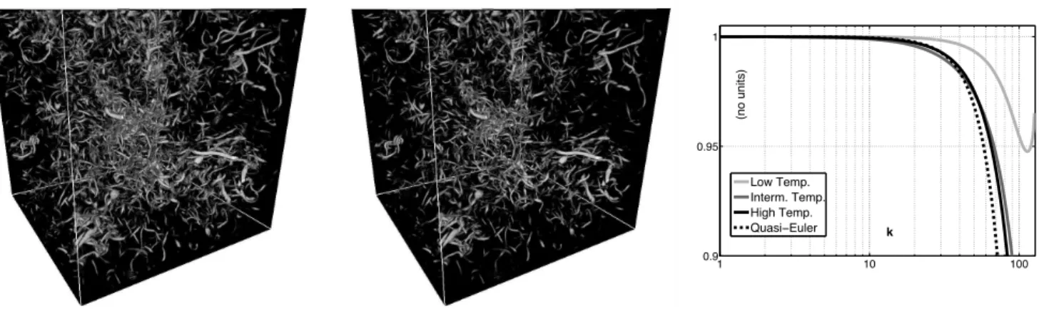
The locking of the two fluids. Figure 1 shows the local superfluid and normal fluid enstrophies |ωs|
2
(left) and |ωn|
2
(right) at the intermediate temperature (ρn = ρs).
Intense vortex regions (“worms”) are highlighted by the colour scale, which becomes gray above 5 < |ωs|
2
> and opaque white above 10 < |ωs|
2
>, where the symbol < · · · > indicates volume averaging 3
. The figure clearly shows that the vorticity structures of the two fluids are very similar. The degree of similarity can be quantified by the correlation coefficient
c1= < ωsωn> √ < ωs 2>< ω n 2>, (4)
We find that c1is larger than 97% at all three
tempera-tures explored, in agreement with recent numerical calcu-lations [23] of a superfluid vortex tangle driven by a turbu-lent normal fluid at high temperature (ρn/ρs≃ 3). Unlike
our work, these simulations ignored the back–reaction of the vortex tangle onto the normal fluid.
The plot on the right side of Fig. 1 compares the spectral coherence function
c2(k) = |v
n(k).vs(k)|2
|vn(k)|2.|vs(k)|2
(5) of superfluid and normal fluid velocity fields: The fact that c2(k) is larger than 98% at all scales below kmax/4, where
kmax = 128 is the largest wave vector associated with
2more than 99.8% of the injected kinetic energy was dissipated
by the normal fluid
3This visualisation was generated with “Vapor” freeware,
1 10 100 0.9 0.95 1 k (no units) Low Temp. Interm. Temp. High Temp. Quasi!Euler
Fig. 1: Left and Center visualisations : local enstrophy (squared vorticity) field of superfluid (left) and normal fluid (center) at intermediate temperature. The pattern of vorticity structures is the same in both fluids, but is more intense in the superfluid. The grayscale is defined in the text. Right plot : Spectral coherence function c2(k) of normal and superfluid velocity fields.
our 2563
mesh, means that superfluid and normal fluid velocity fields are strongly locked along the inertial range, up to the forcing length scale, where the energy, which is injected into one fluid only, is redistributed very efficiently over both fluids. We recall that energy is injected into the normal fluid only, except at low temperature, where it is injected in the superfluid only.
1 10 100 10!6 10!4 k E(k) 10!3 10!2 E | ! s | (k)
Low Temp. : superfluid Low Temp. : normal fluid Low Temp. : slip velocity Interm. Temp. : superfluid Interm. Temp. : normal fluid Interm. Temp. : slip velocity High Temp. : superfluid High Temp. : normal fluid High Temp. : slip velocity Quasi!Euler : superfluid Quasi!Euler : normal fluid Quasi!Euler : slip velocity !5/3
b a
Fig. 2: [colour online] Subplot a : Spectra of the magnitude of the superfluid vorticity |ωs| vs wavenumber k. From top to bottom low [green], intermediate [blue] and high [red] temper-atures. Subplot b / Upper part: Superfluid (thick solid lines) and normal fluid (thick dashed lines) velocity power spectra vs wavenumber k at the three temperatures. The thin dashed line denotes the Kolmogorov k−5/3scaling. Subplot b / Lower part: The thin solid lines show the spectra of the slip velocity at the three temperatures.
The upper set of curves of Fig. 2b presents the super-fluid and normal velocity power spectra En(k) and Es(k)
(defined by Ei=REi(k)dk (i = n, s) where Eiis the total
energy in arbitrary units) at high, intermediate and low temperature. As expected from the previous figure, the
spectra overlap along the inertial range; around k = 10, both spectra are compatible with Kolmogorov’s k−5/3
in-ertial range scaling (illustrated by the thin straight line). Note also that at each temperature, since νs < νn, for
increasing k the normal fluid becomes damped before the superfluid. This is consistent with Fig. 1, which shows that the superfluid enstrophy is indeed stronger than the normal fluid’s.
The slip between the two fluids. If the two fluids were perfectly locked, the mutual friction would be zero, which would inevitably result in the unlocking of the two fluids, as they would experience different forcing and dissipation processes. A residual slip velocity vns= vs− vn between
the two fluid must therefore be present. The lower set of curves in Fig.2b shows the spectrum of vns. The peak
at k ≈ 2 is caused by the forcing, which is applied to a single fluid, and induces a residual slip at this wavevector. The striking feature of this spectrum is that it increases with k in the inertial range, starting at k ∼ 10, and peak-ing in the dissipation scales, where the dissipation of one fluid is significantly larger than that of the other. The in-crease with k of the slip velocity spectrum is remarkably pronounced in the “quasi-Euler” case.
Energy transfer between the two fluids. We focus on the high temperature “quasi-Euler” case (νn/νs = 100,
ρn/ρs= 10) because it is expected to mimic He II
hydro-dynamics more closely than other viscosity ratios. The scale–by–scale energy budget per mass unit for the nor-mal fluid and superfluid are respectively:
∂En ∂t (k, t) = −Dn(k, t) − Tn(k, t) − Mn→s+ ǫ injδ k,2, (6) ∂Es ∂t (k, t) = −Ds(k, t) − Ts(k, t) − Ms→n, (7) where Dnand Ds are the viscous dissipation terms in the
normal fluid and superfluid,
P.-E. Roche1, C.F. Barenghi2E. Leveque3
Tn and Tsare the energy transfer rates arising from triad
interactions between Fourier modes within each fluid; the energy flux at wave number k related to the non-linear interaction is defined by
Fi(k, t) =
Z k 0
Ti(k′, t)dk′. (9)
Ms→n and Mn→s result from the exchange of kinetic
en-ergy between the two fluids by mutual friction : Mn→s(k, t) = −ρs ρ(Fns· vn)(k, t), (10) Ms→n(k, t) = ρn ρ (Fns· vs)(k, t). (11) 3 10 100 0 x 10!5 k
spectral density of energy flux
Triadic term : T s Triadic term : T n Coupling term : M s !> n Coupling term : M n !> s Dissipation term : D s Dissipation term : D n
Algebraic sum : superfluid Algebraic sum : normal fluid
Fig. 3: [colour online] Energy exchange between fluids in the high temperature “quasi-Euler” case ( ρn/ρs= 10 and νn/νs= 100).
Dissipations, triadic interactions and mutual coupling terms in k space are shown in Figure 3. As expected from the stationary of the flow, for each fluid the sum of all terms is close to zero, except at the lowest k (for which volume averaging is not performed over enough in-dependent realisations due to the limited time scale of integration). In the inertial range and in the near dissi-pative range, the triadic interaction terms for both fluids are the same at first order, as expected from vn ≃ vs.
In the normal fluid, the triadic term is roughly compen-sated by the viscous dissipation. In the superfluid, the viscous dissipation is νn/νs = 100 times smaller, and
the triadic term is compensated instead by the coupling term. For consistency, we check that this coupling has a second order effect on the normal flux budget: we find |Mn→s/Ms→n| ≃ ρs/ρn = 0.1. We conclude that in the
inertial range at high temperatures: the slip velocity al-lows energy to leak from the superfluid with a flux which mimics the normal fluid viscous dissipation, so that both fluid end up with similar behaviour. This process remains compatible with a strong locking of the 2 fluids in the limit of high Reynolds numbers.
The dissipation cut–off in the two–fluids cascade. In ordinary Navier-Stokes homogeneous turbulence, the vis-cous cut–off scale η is determined by the energy injection ǫ at large scale d0 and by the kinematic viscosity ν:
η4≈ ν
3
ǫ . (12)
With the exception of the “quasi-Euler” case, the spec-tra of vnand vsare computed with the same viscosities νn
and νsand the same total energy injected per unit volume
at wavenumber k ≃ 2. The collapse of all spectra onto the same curve at low k shown in Fig. 2b indicates that the energy injected is efficiently redistributed between the two fluids, and that both fluids have the same integral scale d0 (as evident in Fig.1). Contrary to what happens in
single–fluid Navier-Stokes turbulence, Fig. 2b shows that the superfluid and normal fluid cutoff–scales are temper-ature dependent: it is apparent that the lower is T , the more extended is the inertial range cascade. Therefore, if one defines the Reynolds number using the classical re-lation with the ratio of large and small scales of the cas-cade, Re = (η/d0)−4/3, one finds that Re is temperature
dependent. Evidently, ordinary turbulent relations such as Eq.12 are not valid in our two–fluids system.
We now argue that the temperature dependence of η and Re observed for finite νs will be present in the limit
νs = 0, and will reflect the temperature-dependent
effi-ciency of the energy transfer from the superfluid to the normal by mutual friction. This process is independent of νn, and more generally is independent of the dissipation
mechanism in the normal fluid. It can be accounted by a temperature-dependent effective superfluid viscosity νef f.
As a starting point, we note in Fig. 2b that at small enough scales |vn| << |vs|. At these small scales the
mutual friction force in the equation for vssimplifies to
−ρρnFns= −
ρn
ρ B
2|ωs|(vn− vs) ≈ α|ωs|vs, (13)
where α = ρnB/(2ρ) [18]. In our model, the prefactor |ωs|
in the mutual friction accounts for the local absolute vor-ticity of the vortex tangle, which, following Ref. [9], can be related to the vortex line density by |ωs| = κL. If the
vor-tex lines are smooth on length scales of order ℓ ≈ L−1/2,
the quantity ℓ measures the inter-vortex spacing and cor-responds to the cut-off scale of superfluid turbulence. We conclude that at sufficiently small scales
−ρρnFns≈ ακLvs≈ νef f(
vs
ℓ2). (14)
where the analogy between vs/ℓ2 and the magnitude of
∇2v
shas suggested the introduction of an effective
super-fluid viscosity:
This effective viscosity is relevant at scales smaller or equal to l, at which superfluid energy is transferred into the normal fluid by mutual friction.
When comparing our DNS model to experiments we must remember that in our continuous model the iden-tification L = |ωs|/κ neglects random vortex filaments
and Kelvin waves of wavelength shorter than ℓ (which be-come particularly important at very low temperatures), thus underestimating the vortex line density. It is there-fore more proper to relate ℓ not to the total L−1/2 but to L−1/2k , defined in our previous paper [16] as the vor-tex line density associated with the polarised part of the vortex tangle. Eq. 15 thus becomes
νef f = L
Lk
ακ (16)
where the ratio L/Lk >1 is expected to be of order one
at high temperature and possibly significantly larger than one in the limit T → 0. This ratio measures the wiggleness of the tangle at small scale, and can be interpreted as a measure of its fractal dimension [26].
0 0.5 1 1.5 2 10!3 10!2 10!1 100 T (K) ! eff / "
Fig. 4: [Colours online]. Effective kinematic viscosity in units of κ. Isolated symbols: Superfluid effective viscosity defined by ν′
ef f = ǫ/(κL) 2
and measured in decaying turbulence experi-ments; [blue] diamonds [5], [red] circles [27], [green] squares [8] and triangles [28, 29]. Lines: analytical models; thick [black] line: present model (Eq.16) with prefactor L/Lk= 2 ( isolated bullet [black] for L/Lk = 30), thin [purple] continuous line: µ/(ρκ) where µ is the dynamic viscosity of the normal fluid; dashed [grey] lines: microscopic model Eq. 66 from Ref. [9] computed with prefactor R0/a0= 106
and 104
An alternative derivation of an effective superfluid vis-cosity has been proposed in Ref. [9] (page 216) from the more microscopic point of view of the friction of individual vortex lines. Fig.4 shows that our macroscopic model of νef f (thick black line) is in excellent agreement with the
microscopic model of Ref. [9](thin grey dashed lines). In the figure our model is plotted with a wiggleness prefactor L/Lk= 2, and the model of Ref. [9] contains a logarithmic
prefactor which has been estimated for two different sets of parameters for laboratory turbulent flows.
Another (experimental) definition of effective superfluid viscosity ν′
ef f = ǫ/(κL)
2 has been proposed in recent
studies of decaying turbulence experiments [5, 8, 27–29]. These values of ν′
ef f are shown in Fig.4 as symbols. The
agreement between νef f and νef f′ is good. Since B is
approximately constant with temperature above 1K, the strong temperature dependent of the effective viscosity arises from the temperature dependence of ρn/ρ, which
suggests that the ratio L/Lk has little temperature
de-pendence above 1K.
Although what happens below 1 K goes beyond the scope of this study, we remark that there is a qualitative good agreement between experimental data below 1K and the low temperature extrapolation of the predicted effec-tive viscosity. A wiggliness prefactor L/Lk ≃ 30 would
allow to account for the measured effective viscosity down to 750 mK typically. This suggests that the cross-over be-tween zero-temperature and finite temperature quantum turbulence occurs at a lower temperature than the usual estimation of 1 K based on phonon (normal fluid) mean free path considerations. In other words, it suggests that a relative small concentration of normal fluid (significantly lower than 1 percent) still produces a dissipation which is comparable to other effects (Kelvin waves cascade, vortex reconnections) which are specific of the superfluid. Al-though our continuous model is no longer justified for the normal fluid below 1 K, this observation is not inconsistent with it, because νef f is derived regardless of the normal
fluid dynamics.
Finally, we speculate on the form of the classical Eq.12 for superfluids. Following the analogy between the mutual friction at small scale and the viscous dissipation (Eq.14), the kinetic energy which is “removed” from the superfluid at small scales is
ǫ ≈ νef f(
v2 s
ℓ2). (17)
Substituting vs≈ κ/ℓ. into Eq.17, we recognise the
al-ternative definition ν′
ef f. Combining Eq.17 and Eq.16, we
obtain the following superfluid counterpart of the classical Eq.12: ℓ4= (ρn ρ B 2) κ3 ǫ L Lk =ακ 3 ǫ L Lk , (18)
where the wiggleness parameter L/Lk is of order one for
T > 1 K and possibly larger at lower temperatures. Note that Eq. 18 contains an implicit temperature dependence through B and ρn/ρ (and possibly through L/Lk in the
low temperature limit).
A quantitative comparison of Eq. 18 with our numer-ical simulations is impossible due to the finiteness of νs
in particular, but we find a good qualitative agreement. Eq. 18 allows us to predict the temperature dependence of the depth of the turbulent cascade, and to define a ”su-perfluid Reynolds number” using the separation of large
P.-E. Roche1, C.F. Barenghi2E. Leveque3
and small scales.
Conclusion and Perspectives. – We have intro-duced a new two–fluids DNS model to study quantum turbulence in a self–consistent way. The model is based on the continuum approximation, and we have discussed its advantages and limitations. Our numerical results sup-port the current understanding [9] that in quantum tur-bulence the superfluid and the normal fluid are strongly coupled. In addition, our results at high temperature show the slip velocity peaks in the dissipation scales, and that whereas in the normal fluid the triadic interaction is bal-anced by the viscous dissipation, in the superfluid it is balanced by the mutual friction. We have also found that the usual turbulence relation (Eq.12) which relates the cutoff scale to the energy injection at large scale ǫ and the kinematic viscosity ν is not valid in our two–fluids system. Finally, we have found that the energy transfer from the superfluid to the normal fluid does not depend on the normal fluid’s dissipation, but it can be accounted by a temperature–dependent effective superfluid viscosity νef f, which we have calculated and which is in good
agree-ment with other estimates. Using this quantity, we have obtained the superfluid equivalent (Eq. 18) to the classical formula (Eq. 12) which relates the energy injection to the dissipation scale.
In discussing our result we have introduced the wiggle-ness parameter L/Lkwhich is or order one above 1 K but
may be larger at smaller temperatures. We speculate that L/Lkis related to the fractal dimension of the tangle; its
increase in the low temperature limit may explain the sat-uration of νef f for T → 0. Further work will solve this
issue.
In two recent experiments [6, 30], the spectrum of vor-tex line density in turbulent superfluids was found to dif-fer from its classical counterpart: the spectrum of local enstrophy. A proposed interpretation assumes that only the “polarised” contribution of the vortex tangle mimics the classical enstrophy [16]. The present numerical model, which only accounts for the polarised contribution, gives results consistent with this picture : the spectrum of the superfluid vorticity |ωs| (Fig. 2a) is indeed similar to
cor-responding spectra in classical fluids.
Future work will also attempt to test further the pro-posed interpretation [16] by adding to the current DNS two–fluids model an equation for a scalar field field ac-counting for the density of the unpolarised contribution of the vortex tangle. Another important problem to ad-dress is the decay of turbulence, which is receiving much experimental attention.
∗ ∗ ∗
We thank L. Chevillard, P. Diribarne and J. Salort for their inputs. Computations have been performed by us-ing the local computus-ing facilities at ENS-Lyon (PSMN) and at the french national computing center CINES.This
work was made possible with support from the EPSRC (EP/D040892) and the ANR (TSF and SHREK).
REFERENCES
[1] Donnelly, R.J., Quantized vortices in Helium II, Cam-bridge University Press, () 1991
[2] Barenghi, C.F., Donnelly, R.J., and Vinen, W.F., J. Low Temp. Phys., 52 (189) 1983
[3] Maurer J., and Tabeling P., Europhys. Lett., 1 (29) 1998
[4] Smith, M. , Hilton, D. and VanSciver, S.W., Phys. Fluids, 11 (751) 1999
[5] Stalp, S.R., Niemela, J.J, Vinen, W.J. and Donnelly, R.J., Phys. Fluids, 14 (1377) 2002
[6] Roche P.-E. et al., Europhys. Lett., 77 (66002) 2007 [7] Vinen, W.F, Proc. Roy. Soc. London, 243 (400) 1958 [8] Chagovets, T. V. and Gordeev, A. V. and Skrbek,
L., Phys. Rev. E, 76 (027301) 2007
[9] Vinen W. F., and Niemela J. J, J. Low Temp. Phys., 128(167) 2002
[10] Hall, H.E., and Vinen, W.F., Proc. Roy. Soc. London, A238(204) 1956
[11] Bekarevich, I.L. and Khalatnikov, I. M., Sov. Phys. JETP, 13 (643) 1961
[12] Henderson, K.L. and Barenghi, C.F., Europhys. Let-ters, 67 (56) 2004
[13] Barenghi, C.F. and Jones, C.A., J. Fluid Mech., 197 (551) 1988
[14] Barenghi, C.F., Phys. Rev. B, 45 (2290) 1992
[15] Barenghi, C.F. and Jones, C.A., J. Fluid Mech., 283 (329) 1995
[16] Roche, P.-E. and Barenghi, C.F., Europhys Lett., 81 (36002) 2008
[17] Merahi, L. and Sagaut, P. and Abidat, Z., Europhys. Letters, 75 (757) 2006
[18] Schwarz. K.W., Phys. Rev. B, 38 (2398) 1988
[19] Kivotides, D., Barenghi, C.F. and Samuels, D.C., Science, 290 (777) 2000
[20] Barenghi, C.F., Bauer, G.H., Samuels, D.C. and Donnelly, R.J., Phys. Fluids, 59 (2117) 1997
[21] Kivotides, D., Vassilicos, J.C., Barenghi, C.F. and Samuels, D.C., Europhys. Lett., 57 (845) 2002.
[22] Kivotides, D., Phys. Rev. B, 76 (054503) 2007
[23] Morris, K., Koplik, J., and Rouson, D.W.I., Phys. Rev. Lett., 101 (015301) 2008
[24] L´evˆeque, E., and Koudella, C. R., Phys. Rev. Lett., 86(4033) 2001
[25] Donnelly, R.J. and Barenghi, C.F., J. Phys. Chem. Ref. Data, 27 (1217) 1998
[26] Kivotides, D., Barenghi, C.F. and Samuels, D.C., Phys. Rev. Lett., 87 (155301) 2001
[27] Niemela, J. J., Sreenivasan, K.R. and Donnelly, R.J., J. Low Temp. Phys, 138 (537) 2005
[28] Walmsley, P. M.,Golov, A. I., Hall, H. E., Levchenko, A. A. and Vinen, W. F., Phys. Rev. Lett., 99(265302) 2007
[29] Walmsley, P. M. and Golov, A. I., Phys. Rev. Lett., 100(245301) 2008
[30] Bradley, D. I. et al., Phys. Rev. Lett., 101 (065302) 2008