Comprehensive comparative analysis
of 5#-end RNA-sequencing methods
The MIT Faculty has made this article openly available.
Please share
how this access benefits you. Your story matters.
Citation
Adiconis, Xian et al. “Comprehensive comparative analysis of
5#-end RNA-sequencing methods.” Nature methods 15 (2018): 505-511
© 2018 The Author(s)
As Published
10.1038/S41592-018-0014-2
Publisher
Springer Nature
Version
Author's final manuscript
Citable link
https://hdl.handle.net/1721.1/125055
Terms of Use
Article is made available in accordance with the publisher's
policy and may be subject to US copyright law. Please refer to the
publisher's site for terms of use.
Comprehensive comparative analysis of 5’ end RNA sequencing
methods
Xian Adiconis#1,2, Adam Haber#1, Sean K. Simmons#2, Ami Levy Moonshine3, Zhe Ji1,
Michele A. Busby3, Xi Shi2, Justin Jacques2, Madeline A. Lancaster4, Jen Q. Pan2, Aviv Regev1,3,5,6,*, and Joshua Z. Levin1,2,*
1Klarman Cell Observatory, Broad Institute of MIT and Harvard, Cambridge, Massachusetts USA 2Stanley Center for Psychiatric Research, Broad Institute of MIT and Harvard, Cambridge,
Massachusetts USA
3Broad Institute of MIT and Harvard, Cambridge, Massachusetts USA 4Medical Research Council, Laboratory of Molecular Biology, Cambridge UK
5Department of Biology, Howard Hughes Medical Institute, Massachusetts Institute of Technology,
Cambridge, Massachusetts USA
6The David H. Koch Institute for Integrative Cancer Research at Massachusetts Institute of
Technology, Department of Biology, Massachusetts Institute of Technology, Cambridge, Massachusetts USA
# These authors contributed equally to this work.
Abstract
RNA-Seq is an effective method to study the transcriptome, but specialized methods are required to identify 5’ ends of transcripts. Several published strategies exist for this specific purpose, but their relative merits have not been systematically analyzed. Here, we directly compare the
performance of six such methods – testing five with cellular RNA as well as a novel spike-in RNA assay that helps address interpretation challenges that arise from uncertainties in annotation or RNA processing. Using a single human RNA sample, we constructed and sequenced 18 libraries with these methods and one standard, control RNA-Seq library. We find that the CAGE method performed best for mRNA and that most of its unannotated peaks are supported by evidence from other genomic methods. We then applied CAGE to eight brain-related samples and revealed sample-specific transcription start site (TSS) usage as well as a transcriptome-wide shift in TSS usage between fetal and adult brain.
Users may view, print, copy, and download text and data-mine the content in such documents, for the purposes of academic research, subject always to the full Conditions of use:http://www.nature.com/authors/editorial_policies/license.html#terms
*Corresponding author: Correspondence should be addressed to J.Z.L. ([email protected]) or A.R. ([email protected]).
AUTHOR CONTRIBUTIONS
J.L, X.A., and A.R. conceived the research. X.A. prepared the 5’ end RNA-Seq libraries. J.J. prepared the standard RNA-Seq library. X.S. prepared the in vitro neurons under the supervision of J.P. M.L. prepared the brain organoid RNA. A.H, S.S., A.L.M., Z.J., and M.B. developed and performed computational analysis. J.L., X.A., A.H., S.S., and A.R. wrote the paper. All authors assisted in editing the paper.
HHS Public Access
Author manuscript
Nat Methods
. Author manuscript; available in PMC 2018 December 04.Published in final edited form as:
Nat Methods. 2018 July ; 15(7): 505–511. doi:10.1038/s41592-018-0014-2.
A
uthor Man
uscr
ipt
A
uthor Man
uscr
ipt
A
uthor Man
uscr
ipt
A
uthor Man
uscr
ipt
INTRODUCTION
Precise promoter annotation is central to addressing many questions in biology, including condition and tissue specific gene regulation, differential 5’ untranslated region usage, and the impact of genetic variation in non-coding regions on gene expression. In particular, as Genome Wide Association Studies and sequencing studies identify thousands of loci associated with human diseases in non-coding regions, the challenge is to relate genetic variants to their mechanism of action1, 2. A critical step for understanding the functional impact of such genetic polymorphisms is correctly identifying transcription start sites (TSSs). For example, a single nucleotide polymorphism in a regulatory region was shown to create a new TSS that interferes with normal activation of downstream alpha-like globin genes, thereby causing thalassemia3. Additionally, identifying multiple TSSs for a gene and understanding their usage in the relevant tissues can help design follow up experiments. Further, in many cases differential TSS usage is important for gene function and in human disease4, such as TP73, where transcription from one promoter leads to a protein acting as a tumor suppressor and the other a protein acting as an oncogene5 and NRXN1 in which mutations found in neurodevelopmental disorder patients have differing symptoms that may reflect the disruption of the alpha and beta promoters6.
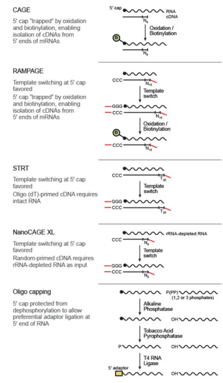
While transcriptome analysis by RNA-Seq is a powerful approach for gene expression measurements, novel transcript discovery, and splice-isoform determination7, it is still often difficult to reliably identify more than one TSS per gene in a given transcript isoform. Empirical determination of the correct TSS in a given sample is particularly important in complex transcriptomes, such as human, where 54% of genes are currently annotated as having multiple TSSs8. Several methods have been proposed for the identification of the 5’ end of transcripts, including CAGE9, RAMPAGE10, 11, STRT12, NanoCAGE13, 14, Oligo Capping (also known as TSS-Seq)15, 16, and GRO-cap17 (also known as 5’ GRO-Seq18) (Fig. 1), but their relative merits have not yet been systematically compared19. Even for a widely accepted method such as CAGE, there are many reads aligning to 3’ rather than 5’ ends of transcripts20, so that further investigation could be beneficial.
Here, we compare six 5’ RNA-Seq methods using a comprehensive set of metrics. Starting from total RNA from one human cell line, we constructed a set of libraries for five of the methods, as well as a control library with standard RNA-Seq, and deeply sequenced them. We identify the CAGE method as performing best for mRNA and show that most of its unannotated TSS peaks also have corroborative evidence to support their being bona fide TSSs. For enhancer RNAs (eRNAs), we find GRO-cap identifies many more transcripts than the other methods. We then used CAGE to generate TSS data for eight brain-related
samples, identifying many examples of differential promoter usage, and showing evidence for a novel, genome-wide trend of differential TSS usage, where downstream TSSs are preferentially used in adult brain and upstream TSSs are used in fetal brain and in vitro differentiated neurons. Our evaluation strategy, results, and brain TSS catalog can serve as resources for the community.
A
uthor Man
uscr
ipt
A
uthor Man
uscr
ipt
A
uthor Man
uscr
ipt
A
uthor Man
uscr
ipt
RESULTS
A comparison of 5’ RNA-Seq methods
We tested five methods for preparing RNA-Seq libraries that identify the 5’ end of transcripts (Fig. 1). We attempted to optimize each method to facilitate efficient library construction and sequencing of indexed libraries on an Illumina sequencing platform (Online Methods). To make a comprehensive comparison, we tested each method by using RNA from the human cell line, K-562, to construct and sequence 18 libraries
(Supplementary Table 1). The methods vary in their input RNA requirements, with STRT, which was developed as an ultra-low input method, requiring the least RNA and Oligo Capping requiring the most (Online Methods). We varied the RNA input by method specifications, but aimed to use the lowest recommended amount, recognizing that RNA quantity can be limiting in practice. To assess whether the lower RNA input amount for STRT compared to the other methods affected its performance, we constructed and sequenced an additional set of eight STRT libraries with input amounts ranging from 10 ng to 10 μg (Supplementary Table 1). In addition, we compared published data for K-562 prepared with GRO-cap17. We constructed one control library using standard RNA-Seq with ribosomal RNA (rRNA) depletion by the RNase H method19, 21 to understand the value of using one of these more specialized RNA-Seq methods.
We first assessed performance of each method by standard RNA-Seq metrics
(Supplementary Table 1). CAGE and NanoCAGE-XL produced fewer reads per library because of limited quantities of library DNA for CAGE and poor sequencing yield for NanoCAGE-XL. All methods showed acceptable levels of reads aligning to rRNA (<20% of reads) and excellent strand specificity (>99% correct strand reads) with the exception of GRO-cap (90% correct strand reads). GRO-cap also had a much higher fraction of reads aligning to introns (20%) and intergenic regions (47%) than the other 5’ end RNA-Seq methods.
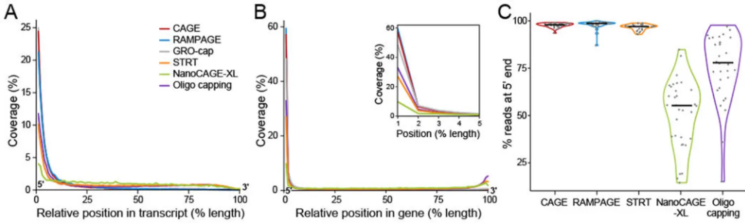
For an initial assessment of specificity for 5’ ends, we examined coverage of reads from 5’ to 3’ (Fig. 2a,b). When considering only reads that aligned to exonic regions, we observed GRO-Cap performed best, followed by CAGE and RAMPAGE and NanoCAGE-XL performed worst (Fig. 2a). Analyzing reads aligning to the entire gene including introns, we observed that RAMPAGE and CAGE performed best followed by GRO-cap (Fig. 2b) – likely reflecting the high fraction of GRO-cap reads aligning to introns (Supplementary Table 1). This global analysis is congruent with our observations for representative highly-expressed genes (Supplementary Fig. 1). Overall, even the best performing method, CAGE, has a sizeable fraction of reads (24% of reads for the average gene) mapping to regions not close to transcript 5’ ends (farther away than 10% of the length of the transcript) by this measure (Fig. 2a).
Assessment of 5’-end specificity with synthetic spike-in RNAs
We next explored why many reads were not aligned at the annotated 5’ end of transcripts (Fig. 2a). Such non-5’ end reads could reflect either technical limitations, incomplete annotation, or biological explanations like RNA re-capping22. To focus on technical
A
uthor Man
uscr
ipt
A
uthor Man
uscr
ipt
A
uthor Man
uscr
ipt
A
uthor Man
uscr
ipt
performance, we developed a spike-in RNA assay using ERCC transcripts23 (Online Methods).
The methods showed similar relative performance based on 5’ end coverage of these artificial transcripts (Fig. 2c and Supplementary Table 2) as with cellular RNA (Fig. 2a), with CAGE and RAMPAGE performing best. STRT performance did not improve with increased input amounts (Supplementary Table 2). The 5’ end specificity differs among the spike-in transcripts – indicating that there is some variability in method performance for different transcripts.
We also assessed how accurately these methods quantitated the relative fraction of each ERCC spike-in transcript. This is important for quantifying differences in TSS usage across samples. For each transcript, we compared the relative input amount to the fraction of reads aligned (Supplementary Table 3). We assessed the uniformity of read coverage using the mean quantitation error (Supplementary Table 4). The CAGE libraries had the lowest error (1.1%) and performed better than RAMPAGE (2.0%).
TSS peak calling to help assess 5’ specificity
To better compare the 5’ specificity of methods for cellular transcripts, we used computational peak calling to identify TSS locations. We reasoned that this would distinguish noisy background reads spread across the length of a gene from peaks of reads aligning to specific locations in that gene. Furthermore, many studies seek to identify TSS peaks and associate them with other genomic and biological information. To enable equivalent comparisons across methods, we randomly sampled 20 million aligned reads for each method, with two exceptions. First, NanoCAGE-XL did not have sufficient reads (Supplementary Table 1), so that we used all its aligned reads. Second, we did not have enough reads from any single CAGE library, and pooled replicate libraries for subsequent analysis. We called peaks from aligned reads using Paraclu24, with parameters optimized for best sensitivity and precision for each library (Online Methods). We also incorporated two additional filtering steps to ensure that our peak calling results accurately represented lab method performance (Supplementary Note 1, Supplementary Fig. 2-4).
CAGE performs best in TSS peak-based comparison
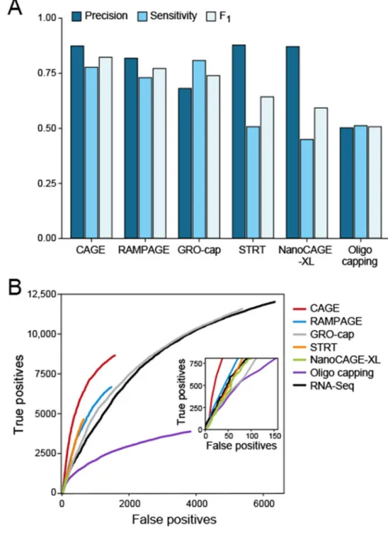
We evaluated each of the six methods for their ability to identify TSSs relative to known annotation. We used the UCSC transcriptome annotation8, which does not rely on data gathered with 5’ end RNA-Seq methods, and as such should not be biased towards any of the methods a priori. For precision, CAGE, STRT, and NanoCAGE-XL performed best (Fig. 3a), while for sensitivity GRO-cap was the best method followed by CAGE and RAMPAGE (Fig. 3a). Combining both considerations, CAGE performed best followed by RAMPAGE, GRO-cap, STRT, NanoCAGE-XL, and Oligo Capping (Fig. 3a,b). STRT performance did not improve with increased input amounts (Supplementary Fig. 5). The same rankings were obtained when using the Gencode annotation25 (Supplementary Fig. 6). In addition, we analyzed published datasets in which two of these methods were tested on the same cell line or tissue in different laboratories. In three cases, we were able to compare CAGE and
A
uthor Man
uscr
ipt
A
uthor Man
uscr
ipt
A
uthor Man
uscr
ipt
A
uthor Man
uscr
ipt
Oligo capping15 (Supplementary Fig. 7).We also compared the performance to 5’ ends identified from standard RNA-Seq (Online Methods). Standard RNA-Seq had more peaks – leading to both more true and false positives – and a ROC curve that suggests a similar false positive to true positive ratio compared to NanoCAGE-XL, which identified the fewest peaks, but worse than all the other 5’ end methods, except Oligo capping (Fig. 3b). For each method, we also assessed TSSs at single base resolution (Supplementary Note 2, Supplementary Fig. 8), reproducibility and gene expression quantification accuracy (Supplementary Note 3, Supplementary Figs. 9,10, Supplementary Tables 2-4).
Evidence supporting unannotated TSS peaks
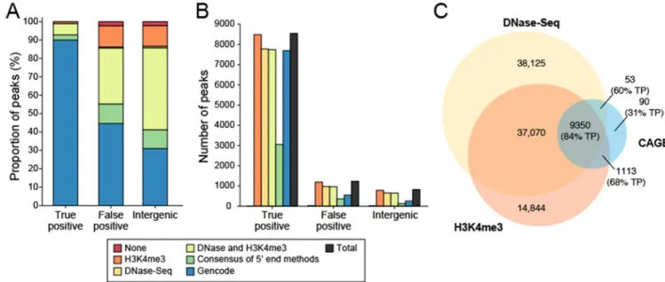
Given that CAGE performed best, we explored its performance further using evidence from other sources. DNase-seq and H3K4me3 ChIP-Seq data can be used to further understand which false positives (based on prior annotation) may actually be true positives. DNase-Seq30 identifies genomic regions with open chromatin such as promoters, and H3K4me3 is associated with TSS regions of active promoters31. While such corroborative data cannot provide a definitive conclusion about which individual peaks are true positives, it adds valuable information about the confidence in each peak.
Indeed, when considering both epigenetic data, Gencode annotations and the consensus peaks identified by the other 5’ end RNA-Seq methods, the vast majority of CAGE peaks have additional support (Fig. 4). First, ~55% of false positive and ~42% of intergenic peaks for CAGE have support from Gencode annotation and/or the consensus peaks identified by the other 5’ end RNA-Seq methods (Fig. 4a). (We omitted NanoCAGE-XL from this consensus because it detected so few peaks (Fig. 3a,b).) Next, with corroborative evidence from DNase-Seq or H3K4me3 ChIP-Seq28, the great majority of the remaining unannotated peaks have some evidence that they may be actual TSSs (Fig. 4a,b). Corroborative evidence for other methods was also analyzed (Supplementary Note 4, Supplementary Fig. 11) Although TSSs are associated with promoters, they can also be found at the start of eRNAs and would be classified as “intergenic” in the annotation we used32, 33. For Paraclu-called peaks found in intergenic regions (Supplementary Fig. 11), we explored their locations relative to enhancer regions in the genome. Using three different approaches based on histone modifications and open chromatin to identify enhancer regions (Online Methods), we observed that GRO-cap had ~5,000 peaks in such regions compared to much fewer such peaks for the other methods (Supplementary Table 5). The percentage of intergenic peaks that were in enhancer regions showed the same trend as for peaks in annotated genes (Fig. 3) with most methods performing well, except for Oligo capping (Supplementary Table 5). Because eRNAs are expressed at lower levels than mRNAs and are expressed as divergent, non-overlapping transcript pairs, we took a second approach based on a previous study33 (Online Methods) to identifying peaks in such regions. We obtained similar results in that GRO-cap had the most TSSs in enhancer regions (Supplementary Table 6).
When considering whether CAGE data are sufficient to identify TSSs in a given sample, it is worth knowing whether collecting corroborative data such as DNase-Seq or H3K4me3 ChIP-Seq can improve the quantity or confidence of the identified TSSs. Figure 4c shows
A
uthor Man
uscr
ipt
A
uthor Man
uscr
ipt
A
uthor Man
uscr
ipt
A
uthor Man
uscr
ipt
how TSS prediction can be refined using such corroborative data together with CAGE data. More CAGE peaks would be filtered out by requiring DNase-Seq than H3K4me3 ChIP-Seq evidence (Fig. 4c). For standard RNA-Seq without CAGE data, the corroborative evidence is even more important in identifying “true positive” 5’ ends, based on annotation, with DNase-Seq evidence again having a bigger impact than H3K4me3 ChIP-Seq (Supplementary Fig. 12).
Differential TSS usage in brain-related samples
Having identified CAGE as best, we applied it to a set of eight brain-related samples to explore differential TSS usage. We selected cell type populations derived from post-mortem brain (neurons, astrocytes, endothelial, and smooth muscle), post-mortem fetal and adult frontal lobe samples, 26 day old in vitro neurons produced with an NGN1 and NGN2 over-expression differentiation protocol34, and 60 day old in vitro brain organoids35. For each sample, we sequenced CAGE libraries, sampled 13 million aligned reads, called peaks using ParaClu, and applied CapFilter (Online Methods). We intentionally focused on differences in TSS usage rather than expression levels (Online Methods) to explore the specific
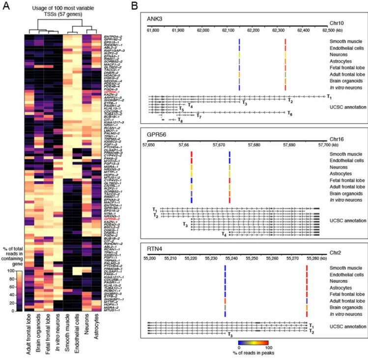
information added by CAGE compared to standard RNA-Seq. Also, we wanted to identify the most significant differences in TSS usage and this can be difficult to discern for genes with low expression in a given sample. To identify TSS peaks differentially used between pairs of samples, for each gene we compared the fraction of reads in a TSS peak between samples. This method identified 2,312 TSS peaks in 1,015 genes that were significantly different (FDR < 0.05, Fisher’s exact test) between at least one pair of these eight samples (Supplementary Table 7). Unsupervised hierarchical clustering of the differentially used TSSs showed relationships among these samples, such as the in vitro models of neuron development being most closely related to the fetal frontal lobe sample (Fig. 5a). For comparison purposes, we also performed unsupervised hierarchical clustering using gene expression levels rather than TSS usage (Supplementary Fig. 13) and observed the resulting clustering of samples is similar to that in Fig. 5a.
Focusing on differences in TSS usage between fetal and adult samples, our analysis highlighted three brain disease-associated genes with differential TSS expression (Fig. 5b). For ANK3, which has been associated with bipolar disorder and schizophrenia36, the T2 (exon 1e37) TSS was more frequently used than the T3 (exon1b37) TSS in all samples, except the adult frontal lobe, consistent with published findings37. For GPR56, the T4 (e1m38) TSS, which has been shown to be the highest expressed TSS in fetal human brain and required for normal human embryonic cerebral cortical development38, was used more frequently in the fetal frontal lobe, in vitro neurons, and brain organoids, but not in the adult frontal lobe, in which T3 was used more often. For RTN4 (also known as NOGO), we observed that the T3 (P2, NOGO-C39) TSS, which was shown to be overexpressed in schizophrenia, was used more frequently in the adult frontal lobe, similar to published studies39, but not in the other samples. For all three genes, TSS usage in adult frontal lobe was more similar to brain organoids than in vitro neurons (Fig. 5b), as might be expected given the more advanced development of the organoids35.
A
uthor Man
uscr
ipt
A
uthor Man
uscr
ipt
A
uthor Man
uscr
ipt
A
uthor Man
uscr
ipt
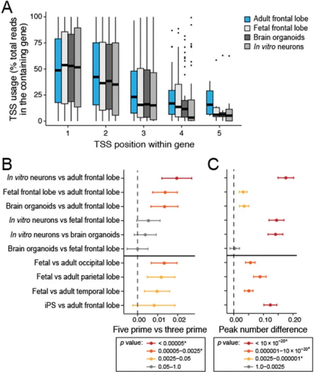
More globally, in vitro neurons, brain organoids, and fetal frontal lobe used an upstream (more 5’) TSS rather than a downstream (more 3’) TSS significantly more often (Bonferroni adjusted P value < 0.05) than adult frontal lobe (Fig. 6a,b). For this comparison, we
computed a scaled average peak position for all genes and datasets, which were compared between samples using a Paired-Wilcoxon signed-rank test (Online Methods). TSS usage was most significantly different between in vitro neurons and adult frontal lobe (Bonferroni adjusted P value = 0.0002) with significant differences also observed between fetal and adult frontal lobe (Bonferroni adjusted P value = 0.0013) and between brain organoids and adult frontal lobe (Bonferroni adjusted P value = 0.023, Fig. 6b). We observed this trend also using FANTOM5 CAGE data from similar samples27 (Fig. 6b). Moreover, the number of TSS per gene was significantly higher (Bonferroni adjusted P value = 2.1*10−32) in the adult fetal lobe than the in vitro neuron or organoid samples from this study as well as in the adult FANTOM5 brain samples compared to the fetal FANTOM5 brain samples (Fig. 6c).
DISCUSSION
We compared six methods for 5’ RNA-Seq by a comprehensive set of quality measures. CAGE performed best overall (Figs. 2 and 3), though other methods might be deployed when less RNA is available. GRO-cap should be considered for identification of eRNA TSSs (Supplementary Tables 5 and 6) but performed worse for mRNA TSSs due a higher rate of false positives (Fig. 3), particularly in genomic regions annotated as introns (Supplementary Table 1). While many peaks identified by GRO-cap could be “real” based on corroborative evidence (Supplementary Fig. 11), it is difficult to judge. Furthermore, GRO-cap is limited to fresh samples and relies on the TAP enzyme, which is no longer commercially available. The methods also vary in the associated time and cost of materials and kits (Supplementary Table 8). The per-sample cost is lowest for STRT and highest for Oligo capping. The amount of time and number of steps per library for each method is lowest for STRT and
NanoCAGE-XL and highest for CAGE.
We aimed to test a fully representative set of the existing methods for 5’ RNA-Seq, but excluded some from our comparisons (Supplementary Note 5).
A key question was which methods were best for annotating TSSs in a sample without previous annotation. Beyond finding that CAGE performed best, we explored how Seq and H3K4me3 ChIP-Seq could refine these assignments (Fig. 4). We found that DNase-Seq and H3K4me3 are insufficient without CAGE to reliably identify TSSs. Moreover, DNase-Seq, but not H3K4me3, does provide additional specificity beyond CAGE. Of course, it is not possible to know with full certainty whether any given TSS identified by these methods is correct. For standard RNA-Seq, DNase-Seq and, to a lesser extent,
H3K4me3, are more valuable in identifying true TSSs based on the annotation, though there are still more false positives with standard RNA-Seq than CAGE even with the corroborative data (Supplementary Fig. 12). ATAC-Seq40 could be substituted for DNase-Seq as the former is simpler with lower input requirements.
Finally, we addressed the question of TSS usage, which is critical for studying disease related genetic variation in non-coding regions, focusing on its relevance to assessing the
A
uthor Man
uscr
ipt
A
uthor Man
uscr
ipt
A
uthor Man
uscr
ipt
A
uthor Man
uscr
ipt
faithfulness of disease models. Human pluripotent stem cells (hPSCs) offer an excellent tool to model human disorders in the lab41, 42, and are particularly relevant for brain-related disorders for which other models are limited43, 44. We compared TSS usage in vitro neurons and brain organoids derived from hPSCs with post-mortem brain samples (Figs. 5 and 6) as it is important to understand how faithfully these models represent actual brain tissue at a transcriptional level. Our results provide a resource for future studies and add to the existing literature in this field27, 45. Brain organoids were more similar than in vitro neurons to adult post-mortem brain samples by our TSS usage measures (Figs. 5a and 6b) – suggesting that the former might be a better model by these criteria. Some of the observed differences are likely explained by post-mortem brain having cell types not found in these in vitro models and potentially changes in RNA abundance due to death-associated cellular responses to hypoxia and other factors46.
With the brain-related samples, we observed a genome-wide trend that relative TSS usage significantly varied with respect to upstream or downstream position within each gene (Fig. 6). Because the size of this effect seems to reflect the overall relatedness of the samples (Fig. 5a) and we identified this pattern in an unrelated CAGE dataset (Fig. 6b), we believe there may be a biological explanation underpinning this result though understanding its basis is beyond the scope of this study. To our knowledge, this phenomenon has not been observed previously, but studies of the 3’ ends of transcripts have shown that upstream
polyadenylation sites are preferentially used in proliferating cells47, while the opposite has been reported in mammalian brain48. Also, a recent paper showed unannotated TSSs were detected upstream of annotated, silenced promoters that may be relevant to aberrant gene expression in cancer due to hypomethylation of these upstream TSSs49.
ONLINE METHODS
RNA samples.
We used the same batch of K-562 total RNA (Thermo Fisher Scientific) in experiments directly comparing the lab methods. For the CAGE, RAMPAGE, and STRT methods, we used a second batch of K-562 RNA (Thermo Fisher Scientific) for comparison to assess method reproducibility. Both batches were high quality RNA, with RNA Integrity Number (RIN) scores of 8.6 and 8.8 as measured with a BioAnalyzer (Agilent).
For the brain-related samples, we used total RNA from each of eight human samples. From ScienCell Research Laboratories, we used brain vascular smooth muscle cell RNA (#1105), brain microvascular endothelial cell RNA (#1005), neuron early passage monolayer culture from fetal brain RNA (#1525), and astrocytes cultured for 6 days from a fetal donor RNA (#1805). From Biochain, we used fetal frontal lobe RNA (#R1244051-50) and adult frontal lobe RNA (#R1234051-50).
We differentiated HUES66 embryonic stem cells, which was created by the Harvard Stem Cell Institute, into neurons by overexpressing NGN1 and NGN234, harvested the cells after 26 days, and isolated total RNA using the Quick-RNA MiniPrep kit (Zymo Research).
A
uthor Man
uscr
ipt
A
uthor Man
uscr
ipt
A
uthor Man
uscr
ipt
A
uthor Man
uscr
ipt
We prepared four brain organoids from a single batch at day 60 of differentiation from H9 embryonic stem cells as previously described50. We isolated total RNA using 1 ml Trizol (Thermo Fisher Scientific) according to the manufacturer’s instructions and isopropanol precipitated with 1 μl GlycoBlue Coprecipitant (Thermo Fisher Scientific). We removed the GlycoBlue, which inhibited the CAGE process, by mixing with 30 μmol LiCl (Sigma) in a total 12 μl and incubating at −20°C for 20 minutes following by centrifugation at 4°C at maximum speed (17,000 × g). We removed the supernatant, rinsed the pellet with 70% ethanol, and re-suspended the pellet in 8.22 μl H2O. We repeated this process one more time until there was no visible GlycoBlue. RIN scores for these 8 samples were 6.8 to 9.7 as measured by BioAnalyzer.
All biospecimens were collected with informed consent. The generation of hES cells used in this study was approved by the institutional review boards (IRBs) of the providing
institutions. Use of all de-identified biospecimens for sequencing at the Broad Institute was further approved reviewed by the Broad’s Office of Research Subject Protection (ORSP), which determined that the research did not involve human subjects according to U.S. federal regulations (45CFR46.102f). This study complied with all relevant ethical regulations.
RNA spike-in controls.
We obtained 32 individual ERCC spike-in controls23 (gift from Jennifer McDaniel and Marc Salit, NIST). We added a m7G cap structure to the 5’ end of RNA molecules using the Vaccinia Capping System (New England BioLabs) following the manufacturer’s protocol. We made a pooled capped ERCC spike-in mix with an average concentration of 36 pg/μl for each transcript. In addition, we prepared a second pooled, capped ERCC spike-in mix with only eight of the transcripts with an average concentration of 138 pg/μl for each transcript. We also made a third pooled original (uncapped) ERCC spike-in mix for all 32 transcripts with average concentration of 60 pg/μl for each transcript.
CAGE libraries.
For K-562 samples, we prepared libraries following a published protocol9 using 10 μg total RNA for three replicates (“Main-1, 4, and 6”) from the same batch of RNA. In a second experiment, we prepared a library with a single replicate (“Repeat”) from 5 μg of a different batch of K-562 RNA. For the brain-related samples, we prepared CAGE libraries from eight total RNAs from sources described above, using between 5 to 10 μg each based on
availability.
For the Main-1, Main-4, and brain-related samples, we added pooled capped ERCC spike-in RNA to each sample in a ratio of 0.128 μl per μg sample input. For the Main-6 sample, we added 1.28 μl pooled, uncapped ERCC spike-in RNA. For the other replicate (Repeat), we added 1.0 μl pooled capped ERCC spike-in mix containing only eight transcripts.
RAMPAGE libraries.
We prepared the libraries following the published protocol11 using 5 μg K-562 total RNA plus 0.64 μl pooled capped ERCC spike-in RNA with the following modifications. (1) We used a universal template switching oligo
5’-A
uthor Man
uscr
ipt
A
uthor Man
uscr
ipt
A
uthor Man
uscr
ipt
A
uthor Man
uscr
ipt
TAGTCGAACTGAAGGTCTCCAGCArGrGrG-3’ instead of the barcoded ones. (2) We used a random 15mer oligo with modified tag sequence for RT to allow index read later on in sequencing 5′-TAGTCGAACGAAGGTCTCCCGTGTGCTCTTCCGATCT(N)15. (3) In the final PCR, we used an 8-base barcoded reverse primer to add index for each individual
library, 5′-CAAGCAGAAGACGGCATACGAGATxrefXXGTGACTGGAGT-3’. (4) We
used a different custom sequencing primer (Supplementary Table 9). We also made a replicate with a different batch of K-562 RNA with 1.0 μl pooled capped ERCC spike-in mix containing only eight transcripts.
STRT libraries.
We synthesized cDNA from 10 ng K-562 total RNA plus 0.64 μl 1/500× dilution of pooled original, uncapped ERCC spike-in RNA following a published protocol12, combined with reverse transcription-PCR conditions based on SMART-Seq251 and the following
modifications. (1) We used a 5’ biotin blocked dT oligo that contains a SalI restriction site (shown as underlined), 5′-/5Biosg/CTACACGACGCTCTTCCGATCTGTCGACT(30)VN– 3’. (2) We used a 5’ template switching oligo (TSO) containing an Illumina adaptor sequence, 5′-CUACACGACGCUCUUCCGAUCUNNNNNGGG – noting all bases are RNA. We made this switch because this oligo is compatible with HiSeq2500, MiSeq, and NextSeq sequencers (lllumina), while the original one12 requires a custom sequencing primer with an annealing temperature that is only suitable for the HiSeq2000. (3) We used a PCR primer with sequence compatible to dT oligo and 5’ TSO, 5
′-CTACACGACGCTCTTCCGATCT-3′, for cDNA amplification. We then eliminated the polyA/T end of the double stranded cDNA by mixing with 1x CutSmart buffer, 10 units of SalI (New England BioLabs) and heating at 37⁰C for 60 minutes. We purified this product by using 0.7x volume AMPureXP SPRI beads (Beckman Coulter Genomics) following vendor protocol. We made the sequencing library with a modified NexteraXT (Illumina) protocol52 with the following modifications in addition. (1) We used 0.125 ng cDNA in ½ volume of a standard NexteraXT reaction. (2) We used the modified Nextera Index 1 primer, 5′-CAAGCAGAAGACGGCATACGAGATxrefXXGTCTCGTGGGCTCGGAGA*T*G-3′ with phosphorothioate bonds (denoted by *) and inverted end bases for protection; the 8 “X” bases indicate in-line index sequences that enable pooling samples. In the same experiment, we also prepared a library with the same quantities of capped ERCC spike-in RNA and K-562 RNA. We also made a replicate with a different batch of K-562 RNA.
In addition, we constructed STRT libraries using a similar protocol as above with 10 ng, 100 ng, 1 μg, 5 μg and 10 μg K-562 total RNA from the same batch as above together with the same proportion of uncapped ERCC spike-in RNA. We made the following modifications to accommodate the higher inputs. (1) For the 5 μg and 10 μg inputs, we used 4 times as much the volume for the RT reaction. (2) We used 10 μl each of the 10 times diluted first strand cDNA from the 1 μg RNA input, 12.5 times diluted ones from the 5 and 10 μg RNA inputs, into the 50 μl of cDNA PCR amplification reaction. (3) We used a 50 μl reaction volume that contained 40 units of SalI to remove the polyA/T end of the double-stranded cDNAs generated in all the higher input RNA libraries.
A
uthor Man
uscr
ipt
A
uthor Man
uscr
ipt
A
uthor Man
uscr
ipt
A
uthor Man
uscr
ipt
Oligo Capping libraries.
We prepared the library following published protocols16, 53, using 40 μg K-562 total RNA plus 5.12 μl pooled capped ERCC spike-in RNA with the following modifications. (1) We used 0.5 μl glycogen (Roche) as the carrier instead of ethachinmate in the ethanol
precipitation step. (2) We used KAPA HotStart Ready Mix (KAPA Biosystems) instead of GeneAmp PCR kits (PerkinElmer) for PCR amplification. (3) We selected 250 to 600 bp instead of 150 to 250 bp PCR products for sequencing.
NanoCAGE-XL libraries.
We prepared a library using 7.5 μg K-562 total RNA plus 0.96 μl pooled capped ERCC spike-in RNA following the published protocol14 with the following modifications. (1) We used a TSO containing 6-base barcode (marked as xref) followed by 6-base spacer, 5 ′-TAGTCGAACTGAAGGTCTCCAGCAxrefGCTATArGrGrG. (2) We used a modified custom sequencing primer (Supplementary Table 9).
Standard RNA-Seq library.
We prepared a library using 1 μg K-562 total RNA plus 2 μl of 1:100 diluted ERCC spike-in mix 1 (Ambion) using the TruSeq RNA-Seq kit (Illumina) with the following modifications. (1) The rRNA was depleted using the RNase H method19 instead of using oligo (dT) selection. (2) We eluted the rRNA depleted RNA from the SPRI beads using EPF buffer from the TruSeq kit and heated at 70°C for 10 minutes. (3) We used a different set of barcoding indices rather than those in the TruSeq kit for the ligation and final PCR steps.
Sequencing
Libraries were sequenced with either HiSeq2500, MiSeq, or NextSeq machines (Illumina), as detailed in Supplementary Table 9. We used paired-end sequencing for some 5’ end libraries to aid with understanding method performance, but this is not generally required with the possible exception of RAMPAGE. The NanoCAGE-XL library was sequenced with a second unrelated library and spiking in 30% PhiX library and loading at a reduced concentration (7 pM) to overcome monotemplate issues with libraries prepared with this method.
Additional 5’ RNA-Seq datasets
For datasets previously generated by other groups, we downloaded the relevant fastq files (Supplementary Table 10) and used them in our method comparisons. For the STRT data29, we picked 100 random mouse hippocampus cells from the single cell dataset and combined them together into one fastq file before processing.
Read processing and alignment
For 5’ end RNA-Seq, we processed reads by trimming an appropriate number of bases depending on the lab method used (Supplementary Table 1). We aligned reads to either the human genome (Gencode v19) or mouse genome (mm10) with STAR54 (version 2.4.2a) using two-pass mode, and the softclip option to trim reads and otherwise default parameters. We only used read 1, which was derived from the 5’ end of the transcript, for these analyses,
A
uthor Man
uscr
ipt
A
uthor Man
uscr
ipt
A
uthor Man
uscr
ipt
A
uthor Man
uscr
ipt
except when we tested the use of read 2 with the RAMPAGE peak calling pipeline (see below). We generated basic alignment and performance metrics, using
CollectAlignmentSummaryMetrics and CollectRnaSeqMetrics in Picard Tools (https:// github.com/broadinstitute/picard). We analyzed the reads for both these metrics and peak calling analyses, but used BAM files generated by STAR with the hardclip option for the former because Picard did not recognize bases as trimmed with the softclip option. For 5’ vs 3’ end coverage, we sampled 20 million reads from each bam file, except NanoCAGE-XL, for which we used all reads. We performed two types of analyses – one using the entire gene including intronic regions and the other using only the exonic regions. In both cases, we used only the position of the most 5’ end of the read (“read start”). For the analysis of the entire gene, we only used genes greater than 500 bp in length and with Transcripts Per Million (TPM) > 1 as estimated with RSEM. We divided each gene into 100 equal sized bins, and totaled the percent of read starts on the same strand as the gene in each bin on a per gene basis using bedtools55 intersect and post-processing in R. We averaged these percentages over all genes, and plotted the results with ggplot56. For analysis using only the exonic regions, we used a similar approach, except for genes with more than one transcript, we selected the one with the highest TPM for each gene and limited our analysis to transcripts with greater than 500 bp in length and TPM > 1.
For ERCC spike-in analysis, we used the same trimmed reads, except as noted in Supplementary Table 1. We aligned to a version of all 92 of the ERCC spike-in RNA sequences that includes all sequences at the 5’ ends (Supplementary Table 11) using BWA57 and a custom Picard module to parse the aligned BAM file to calculate the coverage at each base of the ERCC spike-in reference sequences.
For standard RNA-Seq data, we aligned untrimmed reads with Tophat58 (version v1.4.1) using default parameters except mate-inner-dist set to 300 and mate-std-diff set to 500, followed by Cufflinks59 (v2.2.1) using the default settings.
Peak calling
To identify TSSs, we used the Paraclu24 peak caller, applied to randomly sampled reads as follows. To compare between methods, we randomly sampled 20 million reads from aligned K-562-derived BAM files using a custom shell script, with the exception of NanoCAGE-XL, for which we used all 6,407,741 reads. For other parts of the analysis (reproducibility, MCF-7, mouse hippocampus, human brain-related data, FANTOM5 data) we sampled to different numbers of reads, as detailed below. We sampled only reads from each BAM file that passed platform / vendor quality checks and were flagged as being a primary alignment. For 5’ end methods, 20 million reads are only from read 1, but for standard RNA-Seq, they are from both reads 1 and 2.
Post-processing of ParaClu peaks
We annotated peaks called by ParaClu with several scores to indicate the confidence for increased read density in that region, which were used to remove low-confidence peaks. The
A
uthor Man
uscr
ipt
A
uthor Man
uscr
ipt
A
uthor Man
uscr
ipt
A
uthor Man
uscr
ipt
peak structure, and therefore merged all overlapping peak regions using the bedtools55 ‘merge’ function. We set the scores for the aggregate peak to the maximum ParaClu score over the set of peaks to be merged. All peak regions wider than 300bp or narrower than 3bp were removed.
To indicate the confidence level for a given peak, ParaClu provides three metrics, D – the ‘density rise’, a measure of the fold change between maximum and minimum read density, and an indicator of signal strength., P – the minimum number of positions within the peak covered by reads, and S– the total number of reads mapping to the region within the peak. Low-confidence peaks could then be removed by setting threshold values Dmin, Pmin and
Smin for these three values, respectively, and removing peaks that do not pass all three cutoffs. To identify optimal values for these parameters, we tested all combinations of (integer) values for Dmin in [0,10], Pmin in [0,20], and Smin in [0,180], and assessed peak-calling performance using the F1 score (see below). To ensure that each 5’ RNA-Seq method was analyzed optimally, we repeated this procedure to identify the best parameters for each method, and at the different read depths required for all the comparisons in this study: 20 million for 5’ end RNA-Seq lab method comparisons, 7 million for CAGE reproducibility, 5 million for RAMPAGE and STRT reproducibility, and 13 million for brain-related samples, MCF-7, and mouse hippocampus samples. The final filtering parameters used for each dataset are found in Supplementary Table 12.
We assessed the reproducibility of TSS discovery by using bedtools55 ‘intersect’ to compute the pairwise overlap between ParaClu peaks called using BAM files generated from four CAGE replicates. We also compared overlaps for pairs of replicates for RAMPAGE and STRT.
Peak calling from standard RNA-Seq data
To identify TSS using full-length RNA-seq reads, we merged aligned reads from two replicates using samtools60 and sampled 20 million reads as described above. With
expressed transcripts identified using Cufflinks59, we annotated the region within 100 bp of the 5’ end of each identified transcript as a TSS peak.
Tag cluster identification
To identify TSSs in enhancer regions and understand narrow vs broad peaks, we used an alternative peak calling method27 that aims to find tag clusters (TCs). For each read, we defined the starting location of that read as the start of a TSS and then merged all such TSS starts within 20 bp on the same strand to get TCs. We discarded TCs with less than 3 reads supporting them or longer than 300 bp. We used CapFilter (see ‘additional filtering steps’ below) for methods that add an extra G (CAGE, RAMPAGE, NanoCAGE-XL and STRT). We defined broad peaks as TC’s > 10 bp in width and narrow peaks as those ≤ 10bp.
Peak calling for enhancers
To identify putative eRNAs in K-562 datasets, we adapted a previously published approach33. In particular, we took all intergenic TCs and discarded TCs that overlapped another TC on the opposite strand. We paired reverse and forward stranded TCs, where the
A
uthor Man
uscr
ipt
A
uthor Man
uscr
ipt
A
uthor Man
uscr
ipt
A
uthor Man
uscr
ipt
reverse stranded TC occurred within < 400 bp of the forward stranded TC, and merged overlapping pairs together avoiding overlap between the reverse and forward stranded TC in each pair. We then filtered out all merged pairs where either the reverse or forward TC had much higher coverage than the other. More specifically, we only kept merged pairs with:
−.8 < Number Reads Reverse TC−Number Reads Forward TCNumber Reads Reverse TC+Number Reads Forward TC < .8
We used the middle point of each of these merged pairs as the center of the putative enhancer, and extended by 200 bp on either side to generate the putative enhancer. We compared these putative enhancers to public H3K27ac ChIP-Seq (peaks downloaded from:
http://hgdownload.cse.ucsc.edu/goldenPath/hg19/encodeDCC/wgEncodeBroadHistone/ wgEncodeBroadHistoneK562H3k27acStdPk.broadPeak.gz), DNase-seq (see Corroborative data), and enhancer region datasets (ENCFF687ZGE) from ENCODE28 and the DENdb database61 (http://www.cbrc.kaust.edu.sa/dendb/) using the bedtools55 intersect function with default parameters. Similarly, we compared the intergenic peaks identified with
ParaClu to each of the above datasets using the same approach to test if the peaks overlapped with eRNA.
Identification of TSS initiator sequences
For identifying the dinucleotide sequences at the start of TSSs (“−1” and “+1”, where +1 is the position of the first transcribed base in a transcript and −1 is the position directly before it in the genome), we used a modification of previously published approaches62, 63. In particular, we took all TCs within 100 bp of an annotated gene and with at least 10 reads mapping to them, and located the position in each TC with the largest number of reads starting there. We used this location as the putative start site (the +1 location) for the TC. Note that for methods that add an extra G (CAGE, RAMPAGE, NanoCAGE-XL and STRT), we shifted the putative start site over by one base pair in the 3’ direction. We used bedtools55 to extract the +1 and −1 base for each putative TSS from the human genome and created logos using the ggseqlogo package in R64.
Additional filtering steps
We evaluated three specialized filtering programs: CapFilter14, strand invasion65, and the RAMPAGE10 second read filter (downloaded from http://megraw.cgrb.oregonstate.edu/ software/CapFilter, https://academic.oup.com/nar/article/41/3/e44/2902349/Suppression-of-artifacts-and-barcode-bias-in-high#supplementary-data, http://labshare.cshl.edu/shares/ gingeraslab/www-data/dobin/ENCODEpipelines/ENCODE_longRNApipeline_GIT/DAC/ rampagePeakCaller.py). For CapFilter and strand invasion, we slightly modified the code to allow applications beyond NanoCAGE-XL – the lab method for which they were originally developed. We applied CapFilter to CAGE, RAMPAGE, NanoCAGE-XL, and STRT. In each case, we began by calling peaks as above and then applied CapFilter to the resulting peaks. This led to a smaller set of final peaks. We tested CapFilter with various settings of the thresholding parameter (which corresponds to the percentage of G’s in the first position), and found that a threshold of 20% seemed to be optimal for all experimental methods
A
uthor Man
uscr
ipt
A
uthor Man
uscr
ipt
A
uthor Man
uscr
ipt
A
uthor Man
uscr
ipt
We applied the strand invasion filter65 to the NanoCAGE-XL and STRT data. This filter removes potentially artefactual reads that are the result of strand invasion, where the PCR primer primes at sequences in the cDNA similar to the template-switching oligonucleotide (TSO) rather than in the TSO. By checking for matches between the TSO and the sequence upstream of read 1, such events can be identified and filtered out. Using all the NanoCAGE-XL aligned reads and 20 million sampled STRT aligned reads from the BAM files, we applied the strand invasion filter, varying the maximum allowed edit distance between the TSO and the upstream sequence, before calling peaks with ParaClu. We tested varying this parameter between 0 and 7, both with and without CapFilter. We found that this filter did not improve on CapFilter when used in combination with CapFilter (Supplementary Fig. 3a) and did not include strand invasion in our main analysis.
We compared the RAMPAGE peak caller10 with and without second read filtering to the Paraclu results. Because the RAMPAGE filter did not improve performance CapFilter (Supplementary Fig. 3b), we did not include it in our main analysis.
Accuracy assessment
In order to estimate the accuracy of each method, we looked at the number of peaks that overlapped known TSSs based on the UCSC annotation (see Corroborative data). True positive (TP) peaks were defined as those that overlapped at least one annotated TSS, and false positive (FP) peaks as those that did not overlap any TSSs. Intergenic peaks did not overlap any genes according to the UCSC annotation. False negative (FN) peaks were defined as all annotated TSSs, which were (1) within any gene expressed with TPM >1 (quantified using RSEM66 (v.1.2.7) from 5’ RNA-Seq data), (2) overlapped by at least one DNase-Seq peak (see Corroborative data), and (3) did not overlap any of the peaks called by ParaClu. We calculated the ROC curve for each method based on the peak scores output by Paraclu. We calculated sensitivity, precision, and F1 score according to these formulas.
Precision =TP + FPTP
Sensitivity =TP + FNTP
F1 = 2 Sensitivity∗PrecisionSensitivity+Precision
In all cases, a 100bp tolerance was considered an overlap, implemented using bedtools ‘window’.
For mouse-derived data, we modified the expression estimation pipeline, so that instead of using RSEM with its standard settings to quantify expression when defining false negatives, we first mapped the reads to the mm10 UCSC transcriptome using STAR and then applied RSEM to the resulting bam file. In order to produce a bam file that RSEM could use, STAR
A
uthor Man
uscr
ipt
A
uthor Man
uscr
ipt
A
uthor Man
uscr
ipt
A
uthor Man
uscr
ipt
was run with the options: quantMode TranscriptomeSAM, alignIntronMax 1, --alignIntronMin 2, --scoreDelOpen −10000, and --scoreInsOpen −10000.
Corroborative data
H3K4me3 peaks were originally generated from ChIP-Seq as part of the ENCODE Consortium28. We downloaded peaks from: http://hgdownload.cse.ucsc.edu/goldenPath/ hg19/encodeDCC/wgEncodeBroadHistone/
wgEncodeBroadHistoneK562H3k4me3StdPk.broadPeak.gz.
The associated GEO Accession number is GSM733680. We obtained bam files for K-562 DNase-1 hypersensitivity peaks (DNase-seq) from the SRA database (SRR231254 and SRR231189), called peaks with Macs267 with the --nomodel option and default settings, and selected only peaks found in both replicates, by computing the intersection of the two replicates using bedtools55 ‘intersect’. For the other DNase-seq datasets, we downloaded bed files containing peaks from the ENCODE portal68 (ENCFF408UYX for MCF-7;
ENCFF630GRU for mouse brain).
TSS annotations
Annotated transcription start sites (TSS) were downloaded from the UCSC table browser, accessible at: https://genome.ucsc.edu/cgi-bin/hgTables and Gencode25 annotated transcripts were downloaded from ftp://ftp.sanger.ac.uk/pub/gencode/Gencode_human/release_19/ gencode.v19.annotation.gtf.gz and converted to a bed file containing TSS only by extracting the 5’ end of all transcripts in the .gtf file using a custom shell script.
Coverage of peaks in brain-related samples
We sampled 13 million aligned reads from each brain-related dataset and called peaks with Paraclu and applied CapFilter as above. We combined the resulting peaks from all the samples into one file and merged with bedtools55. This ensures that slight differences in peak calls between samples (due to inherent randomness in the data) do not affect
downstream analysis. We removed all peaks that did not overlap at least one annotated TSS within a tolerance of 100 bp. We used the bedtools coverage command to find the number of reads covering each peak – resulting in a matrix with one column for each sample and one row for each (merged) peak. We also used bedtools to annotate each peak to include the name of the gene in which it was located.
Coverage of peaks in FANTOM5 data
We downloaded FANTOM527 BAM files from fantom.gsc.riken.jp/5. In total we downloaded 12 samples: iPS day 18 of differentiation to neurons69, adult frontal cortex, adult and fetal occipital cortex, adult and fetal parietal cortex, and adult and fetal temporal cortex (Supplementary Table 10).
We processed the iPS and adult frontal cortex data through the same pipeline as our brain-related data, to generate a matrix with one column for each sample and one row for each (merged) peak. We used a similar pipeline for the remaining six samples, except instead of
A
uthor Man
uscr
ipt
A
uthor Man
uscr
ipt
A
uthor Man
uscr
ipt
A
uthor Man
uscr
ipt
million reads for the remaining four samples because there were fewer reads for these samples. In addition, we were unable to apply CapFilter to the FANTOM5 reads because they were already trimmed.
Differential TSS usage
To control for differences in overall gene expression, we computed the relative usage for each TSS i in gene j as Rij= 100 rij
∑i = 1k j rij
, where rij is the number of reads within TSS peak i in gene j and kj is the number of TSSs in gene j. To identify differential usage, we
considered all gene/ sample pairs with > 100 reads, and compared the relative usage (rounded to the nearest integer) for the set of TSSs in a given gene between each pair of samples using Fisher’s exact test implemented using the R function fisher.test in the stats package with default parameters, including alternative=“two.sided.” More specifically, the test was performed on the 2 by kj table with one row per sample and one column per TSS, where the table entries are taken to be the corresponding Rij values (we use Rij values instead of raw counts to help correct for number of reads per gene, resulting in a more conservative test statistic). We then took the minimum P value across all comparisons, Bonferroni corrected for the multiple comparisons per gene, was reported as the P value for differential usage across the samples within a gene. Note that we only compared genes with at least 100 reads mapped to them in the samples of interest. We corrected Fisher P values for multiple hypothesis testing using the Benjamini-Hochberg FDR correction, implemented using the R function p.adjust.
Testing upstream vs. downstream bias in TSS usage
To test if there was an upstream vs. downstream bias in TSS usage between different brain samples, we used the peak by sample matrix generated above. For each gene and each sample, we calculated an average normalized peak score. More formally, for a given gene, if that gene had k peaks 1, 2, …, k (ordered from most to least upstream), and had nij reads covering the j-th peak in the i-th gene, the score for that gene was equal to:
scorei =1kj = 1∑ k
j ∗ nij The larger this score, the more that downstream peaks are used.
We used a Wilcoxon signed-rank test (one-sided) to compare the average normalized peak scores for genes between samples. We correct for multiple testing with Bonferroni correction (a total of 20 tests were made—12 from our brain-related data, 8 from the FANTOM5 data).
Expression analysis
To compare estimated gene expression values between samples (Supplementary Fig. 10), we extracted TPM values from the RSEM results for each 5’ method, as well as from standard
A
uthor Man
uscr
ipt
A
uthor Man
uscr
ipt
A
uthor Man
uscr
ipt
A
uthor Man
uscr
ipt
RNA-Seq. We log normalized these data before calculating the Pearson correlation coefficient, r.
The coloring in each comparison is based on a normalized density. For each pair of samples, this was calculated by removing all genes with TPM = 0 in either sample, and using a 2-D Gaussian kernel-based density estimate, using the kde2d function in the R MASS package70. The density values were normalized to be between 0 and 1, to allow for a shared scale—this enables us to see the relative density around each gene.
Statistics
To compare TSS usage for a given gene between different conditions, we used a Fisher’s exact test (see ‘Differential TSS usage’ for more details). For this test n = 2 (one sample for each condition). In order to test for difference in number of TSS used and 5’ biases between conditions we used a one-sided Wilcoxon signed-rank test (see ‘Testing upstream vs. downstream bias in TSS usage’ for more details), with 95% confidence intervals estimated using a Gaussian approximation. Again, this test uses n = 2 (one sample for each condition). Multiple hypothesis testing was performed for all statistical tests using either Bonferroni or Benjamini-Hochberg FDR correction. All other statistics included in the paper are
descriptive in nature.
Life Sciences Reporting Summary
Further information on experimental design is available in the Life Sciences Reporting Summary.
Code availability
Custom computer code used to generate results that are reported in this study and central to its main claims is freely available at https://github.com/seanken/FivePrime.
Data availability
Sequence data for K-562 libraries are available at Gene Expression Omnibus GSE103486. Sequence data for human brain-related samples are available at dbGaP under accession code phs001463.v1.p1.
Supplementary Material
Refer to Web version on PubMed Central for supplementary material.
ACKNOWLEDGEMENTS
We are grateful to M. Salit and J. McDaniel (National Institute of Standards and Technology) for ERCC spike-in RNA. P. Batut for sharing RAMPAGE peak calling code, N. Shoresh for advice on Epigenomics datasets, N. Sanjana for advice on preparing the NGN1/2 in vitro neuron sample, B. Haas, Y. Farjoun, and M. Hofree for statistical advice, L. Gaffney for assistance with figures, I. Wortman and C. Cheng for K-562 experiments, C. de Boer for helpful comments on this manuscript, and the Broad Genomics Platform for sequencing. We thank S. McCarroll for suggesting this research direction and helpful discussions in the early phases of this study. Work was
A
uthor Man
uscr
ipt
A
uthor Man
uscr
ipt
A
uthor Man
uscr
ipt
A
uthor Man
uscr
ipt
REFERENCES
1. Heinzen EL , Neale BM , Traynelis SF , Allen AS & Goldstein DB The genetics of neuropsychiatric diseases: looking in and beyond the exome. Annu Rev Neurosci 38, 47–68 (2015).25840007 2. Edwards SL , Beesley J , French JD & Dunning AM Beyond GWASs: illuminating the dark road
from association to function. Am J Hum Genet 93, 779–797 (2013).24210251 3. De Gobbi M et al. A regulatory SNP causes a human genetic disease by creating a new
transcriptional promoter. Science 312, 1215–1217 (2006).16728641
4. Davuluri RV , Suzuki Y , Sugano S , Plass C & Huang TH The functional consequences of alternative promoter use in mammalian genomes. Trends Genet 24, 167–177 (2008).18329129 5. Grob TJ et al. Human delta Np73 regulates a dominant negative feedback loop for TAp73 and p53.
Cell Death Differ 8, 1213–1223 (2001).11753569
6. Bena F et al. Molecular and clinical characterization of 25 individuals with exonic deletions of NRXN1 and comprehensive review of the literature. Am J Med Genet B Neuropsychiatr Genet 162B, 388–403 (2013).23533028
7. Hrdlickova R , Toloue M & Tian B RNA-Seq methods for transcriptome analysis. Wiley Interdiscip Rev RNA 8 (2017).
8. Tyner C et al. The UCSC Genome Browser database: 2017 update. Nucleic Acids Res 45, D626– D634 (2017).27899642
9. Murata M et al. Detecting expressed genes using CAGE. Methods Mol Biol 1164, 67–85 (2014). 24927836
10. Batut P , Dobin A , Plessy C , Carninci P & Gingeras TR High-fidelity promoter profiling reveals widespread alternative promoter usage and transposon-driven developmental gene expression. Genome Res 23, 169–180 (2013).22936248
11. Batut P & Gingeras TR RAMPAGE: promoter activity profiling by paired-end sequencing of 5’-complete cDNAs. Curr Protoc Mol Biol 104, Unit 25B 11 (2013).
12. Islam S et al. Highly multiplexed and strand-specific single-cell RNA 5’ end sequencing. Nat Protoc 7, 813–828 (2012).22481528
13. Salimullah M , Sakai M , Plessy C & Carninci P NanoCAGE: a high-resolution technique to discover and interrogate cell transcriptomes. Cold Spring Harb Protoc 2011, pdb prot5559 (2011). 14. Cumbie JS , Ivanchenko MG & Megraw M NanoCAGE-XL and CapFilter: an approach to genome
wide identification of high confidence transcription start sites. BMC Genomics 16, 597 (2015). 26268438
15. Yamashita R et al. Genome-wide characterization of transcriptional start sites in humans by integrative transcriptome analysis. Genome Res 21, 775–789 (2011).21372179
16. Tsuchihara K et al. Massive transcriptional start site analysis of human genes in hypoxia cells. Nucleic Acids Res 37, 2249–2263 (2009).19237398
17. Core LJ et al. Analysis of nascent RNA identifies a unified architecture of initiation regions at mammalian promoters and enhancers. Nat Genet 46, 1311–1320 (2014).25383968
18. Lam MT et al. Rev-Erbs repress macrophage gene expression by inhibiting enhancer-directed transcription. Nature 498, 511–515 (2013).23728303
19. Adiconis X et al. Comparative analysis of RNA sequencing methods for degraded or low-input samples. Nat. Methods 10, 623–629 (2013).23685885
20. Hestand MS et al. Tissue-specific transcript annotation and expression profiling with complementary next-generation sequencing technologies. Nucleic Acids Res 38, e165 (2010). 20615900
21. Morlan JD , Qu K & Sinicropi DV Selective Depletion of rRNA Enables Whole Transcriptome Profiling of Archival Fixed Tissue. PloS One 7, e42882 (2012).22900061
22. Schoenberg DR & Maquat LE Re-capping the message. Trends Biochem Sci 34, 435–442 (2009). 19729311
23. Jiang L et al. Synthetic spike-in standards for RNA-seq experiments. Genome research 21, 1543– 1551 (2011).21816910
A
uthor Man
uscr
ipt
A
uthor Man
uscr
ipt
A
uthor Man
uscr
ipt
A
uthor Man
uscr
ipt
24. Frith MC et al. A code for transcription initiation in mammalian genomes. Genome Res 18, 1–12 (2008).18032727
25. Harrow J et al. GENCODE: the reference human genome annotation for The ENCODE Project. Genome Res 22, 1760–1774 (2012).22955987
26. Djebali S et al. Landscape of transcription in human cells. Nature 489, 101–108 (2012).22955620 27. TheFANTOMConsortium et al. A promoter-level mammalian expression atlas. Nature 507, 462–
470 (2014).24670764
28. EncodeProjectConsortium An integrated encyclopedia of DNA elements in the human genome. Nature 489, 57–74 (2012).22955616
29. Zeisel A et al. Brain structure. Cell types in the mouse cortex and hippocampus revealed by single-cell RNA-seq. Science 347, 1138–1142 (2015).25700174
30. Boyle AP et al. High-resolution mapping and characterization of open chromatin across the genome. Cell 132, 311–322 (2008).18243105
31. Hoffman MM et al. Integrative annotation of chromatin elements from ENCODE data. Nucleic Acids Res 41, 827–841 (2013).23221638
32. Kim TK et al. Widespread transcription at neuronal activity-regulated enhancers. Nature 465, 182– 187 (2010).20393465
33. Andersson R et al. An atlas of active enhancers across human cell types and tissues. Nature 507, 455–461 (2014).24670763
34. Busskamp V et al. Rapid neurogenesis through transcriptional activation in human stem cells. Mol Syst Biol 10, 760 (2014).25403753
35. Lancaster MA & Knoblich JA Organogenesis in a dish: modeling development and disease using organoid technologies. Science 345, 1247125 (2014).25035496
36. Hughes T et al. A Loss-of-Function Variant in a Minor Isoform of ANK3 Protects Against Bipolar Disorder and Schizophrenia. Biol Psychiatry 80, 323–330 (2016).26682468
37. Rueckert EH et al. Cis-acting regulation of brain-specific ANK3 gene expression by a genetic variant associated with bipolar disorder. Mol Psychiatry 18, 922–929 (2013).22850628 38. Bae BI et al. Evolutionarily dynamic alternative splicing of GPR56 regulates regional cerebral
cortical patterning. Science 343, 764–768 (2014).24531968
39. Novak G & Tallerico T Nogo A, B and C expression in schizophrenia, depression and bipolar frontal cortex, and correlation of Nogo expression with CAA/TATC polymorphism in 3’-UTR. Brain Res 1120, 161–171 (2006).17022955
40. Buenrostro JD , Giresi PG , Zaba LC , Chang HY & Greenleaf WJ Transposition of native chromatin for fast and sensitive epigenomic profiling of open chromatin, DNA-binding proteins and nucleosome position. Nat Methods 10, 1213–1218 (2013).24097267
41. Bellin M , Marchetto MC , Gage FH & Mummery CL Induced pluripotent stem cells: the new patient? Nat Rev Mol Cell Biol 13, 713–726 (2012).23034453
42. Sterneckert JL , Reinhardt P & Scholer HR Investigating human disease using stem cell models. Nat Rev Genet 15, 625–639 (2014).25069490
43. Imaizumi Y & Okano H Modeling human neurological disorders with induced pluripotent stem cells. J Neurochem 129, 388–399 (2014).24286589
44. Hyman SE Revitalizing psychiatric therapeutics. Neuropsychopharmacology 39, 220–229 (2014). 24317307
45. Arner E et al. Transcribed enhancers lead waves of coordinated transcription in transitioning mammalian cells. Science 347, 1010–1014 (2015).25678556
46. Birdsill AC , Walker DG , Lue L , Sue LI & Beach TG Postmortem interval effect on RNA and gene expression in human brain tissue. Cell Tissue Bank 12, 311–318 (2011).20703815 47. Sandberg R , Neilson JR , Sarma A , Sharp PA & Burge CB Proliferating cells express mRNAs
with shortened 3’ untranslated regions and fewer microRNA target sites. Science 320, 1643–1647 (2008).18566288
48. Miura P , Shenker S , Andreu-Agullo C , Westholm JO & Lai EC Widespread and extensive
A
uthor Man
uscr
ipt
A
uthor Man
uscr
ipt
A
uthor Man
uscr
ipt
A
uthor Man
uscr
ipt
49. Sarda S , Das A , Vinson C & Hannenhalli S Distal CpG islands can serve as alternative promoters to transcribe genes with silenced proximal promoters. Genome Res 27, 553–566 (2017).28223400 50. Lancaster MA & Knoblich JA Generation of cerebral organoids from human pluripotent stem cells.
Nat Protoc 9, 2329–2340 (2014).25188634
51. Picelli S et al. Smart-seq2 for sensitive full-length transcriptome profiling in single cells. Nat Methods 10, 1096–1098 (2013).24056875
52. Soumillon M , Cacchiarelli D , Semrau S , van Oudenaarden A & Mikkelsen TS Characterization of directed differentiation by high-throughput single-cell RNA-Seq. bioRxiv (2014).
53. Suzuki Y & Sugano S Construction of a full-length enriched and a 5’-end enriched cDNA library using the oligo-capping method. Methods Mol Biol 221, 73–91 (2003).12703735
54. Dobin A et al. STAR: ultrafast universal RNA-seq aligner. Bioinformatics 29, 15–21 (2013). 23104886
55. Quinlan AR & Hall IM BEDTools: a flexible suite of utilities for comparing genomic features. Bioinformatics 26, 841–842 (2010).20110278
56. Wickham H ggplot2: Elegant Graphics for Data Analysis (Use R!), Edn. Second. (Springer, New York; 2009).
57. Li H & Durbin R Fast and accurate short read alignment with Burrows-Wheeler transform. Bioinformatics 25, 1754–1760 (2009).19451168
58. Trapnell C , Pachter L & Salzberg SL TopHat: discovering splice junctions with RNA-Seq. Bioinformatics 25, 1105–1111 (2009).19289445
59. Trapnell C et al. Transcript assembly and quantification by RNA-Seq reveals unannotated transcripts and isoform switching during cell differentiation. Nat. Biotechnol. 28, 511–515 (2010). 20436464
60. Zhang K et al. Digital RNA allelotyping reveals tissue-specific and allele-specific gene expression in human. Nat Methods 6, 613–618 (2009).19620972
61. Ashoor H , Kleftogiannis D , Radovanovic A & Bajic VB DENdb: database of integrated human enhancers. Database (Oxford) 2015 (2015).
62. Carninci P et al. Genome-wide analysis of mammalian promoter architecture and evolution. Nat Genet 38, 626–635 (2006).16645617
63. Zhao X , Valen E , Parker BJ & Sandelin A Systematic clustering of transcription start site landscapes. PLoS One 6, e23409 (2011).21887249
64. Wagih O ggseqlogo: a versatile R package for drawing sequence logos. Bioinformatics 33, 3645– 3647 (2017).29036507
65. Tang DT et al. Suppression of artifacts and barcode bias in high-throughput transcriptome analyses utilizing template switching. Nucleic Acids Res 41, e44 (2013).23180801
66. Li B & Dewey CN RSEM: accurate transcript quantification from RNA-Seq data with or without a reference genome. BMC Bioinformatics 12, 323 (2011).21816040
67. Zhang Y et al. Model-based analysis of ChIP-Seq (MACS). Genome Biol 9, R137 (2008). 18798982
68. Sloan CA et al. ENCODE data at the ENCODE portal. Nucleic Acids Res 44, D726–732 (2016). 26527727
69. Chambers SM et al. Combined small-molecule inhibition accelerates developmental timing and converts human pluripotent stem cells into nociceptors. Nat Biotechnol 30, 715–720 (2012). 22750882
70. Venables WN & Ripley BD Modern Applied Statistics with S. (Springer, New York; 2002).
A
uthor Man
uscr
ipt
A
uthor Man
uscr
ipt
A
uthor Man
uscr
ipt
A
uthor Man
uscr
ipt
Figure 1. Methods for 5’ end RNA-Seq.
Salient details for five protocols tested in this paper. Additional properties of these protocols can be found in Supplementary Table 8.