Eastern enlargement of the EU is a central pillar in Europe’s post-Cold War architecture. Keeping the eastern countries out seriously endangers their economic transition, and economic failure in the east could threaten peace and prosperity in western Europe. The perceived economic costs and benefits will dictate the enlargement’s timing. There are four parts to the calculus – the costs and the benefits in the east and in the west. Here we break new ground in estimating the economic benefits of enlargement for east and west using simulations in a global applied general equilibrium model. Our analysis includes a scenario in which joining the EU significantly reduces the risk premium on investment in the east – with resulting huge benefits to the new entrants. We also review the existing literature on the EU budget costs and arrive at a surprisingly well-determined ‘consensus’ estimate, which we support with a new political economy analysis of the budget. The bottom line is unambiguous and strongly positive: enlargement is a very good deal for both the EU incumbents and the new members.
— Richard E. Baldwin, Joseph F. Francois and Richard Portes
Small costs for the west, big gains for the east
SUMMARY
Economic Policy April 1997 Printed in Great Britain © CEPR, CES, MSH, 1997.
1. INTRODUCTION
Just one decade ago, millions of men and trillions of dollars of equipment stood ready for combat in Europe. The demise of the political systems in eastern Europe and the Soviet Union defused the situation. This political ‘creative destruction’ opened the door to great opportunities, but also to great dangers. On the bright side, a continuing success story in eastern Europe will lock in democracy and pro-market reforms. Moreover, a hundred million eastern consumers with rising incomes are a bonanza for western European businesses. Continuing economic success in the east will foster prosperity and peace throughout the continent. On the dark side, however, stagnant or falling incomes and impoverishment of a large slice of the population could foster widespread disillusionment with market economics and democracy. Most worrying of all is that this may occur while a power vacuum exists in central Europe.
Geography and history make these continent-wide problems. Even without speaking of war, any serious unrest or conflict – even if it were limited to the east – could harm western Europe via mass migrations, increased defence expenditures
The costs and benefits of
eastern enlargement:
the impact on the EU and
central Europe
Richard E. Baldwin, Joseph F. Francois and Richard Portes
Graduate Institute of International Studies, University of Geneva and CEPR; Erasmus University Rotterdam, WTO and CEPR; London Business School and CEPR
and changes in investors’ attitudes. In short, economic failure in the east could threaten peace and prosperity in western Europe.
There is, fortunately, a simple way simultaneously to ensure the bright-side economic outcome and to alleviate the power vacuum – enlarge the European Union to include the ten central and eastern European countries (CEECs): the Visegrad-5 (Czech Republic, Hungary, Slovak Republic, Slovenia and Poland), the Balkan-2 (Bulgaria and Romania) and the Baltic-3 (Estonia, Latvia and Lithuania). In this sense, eastern enlargement is a central pillar in Europe’s post-Cold War architecture. Western European politicians have the power to meet this historic challenge, but contemplation of the economic and financial costs of doing so has led them to procrastinate. In other words, geopolitical considerations constitute the engine driving enlargement, but the economic and financial considerations constitute the brake. This paper looks at the economic costs and benefits of admitting the CEECs into the EU.
There are four parts to the calculus – the costs and the benefits in the east and the costs and the benefits in the west. Unfortunately, efforts to date have been directed almost exclusively to the costs to the EU budget of an eastern enlargement. Moreover, there is a widely held belief that even this limited debate has been inconclusive. For instance, the Financial Times (16 December 1996) quotes an MEP with a leading role in the enlargement debate, Mr Arie Oostlander, as saying that ‘the “wildest rumours” were circulating about the cost of enlargement, while the reality was that “adequate reliable information is not currently available”’. One of the contributions of this article is to argue that a sober evaluation of the literature shows that there is a relatively narrow range of estimates for the budget cost of enlargement. Moreover, this range is quite low compared to the early estimates that stimulated much thinking on the enlargement issue. We believe the estimates below are fairly reliable and indeed adequate for an overall assessment of the economic impact of enlargement.
A second contribution of this article is to fill in two more parts of the calculus: the economic benefits for the east and the west. The final part – the cost of enlargement for the east – seems to defy calculation. The main issue here concerns the extent to which adoption of the European Union’s body of legislation and case law – the acquis – will stunt eastern growth and raise unemployment rates. After all, the EU’s rules were designed for rich social democracies with extensive social security systems. They are thus unlikely to be appropriate for poorer but rapidly growing eastern nations. Imagine what would have happened if Korea, Taiwan and Hong Kong had been forced to adopt Social Charter rules and EU environmental standards at a comparable stage of their development. The CEECs do need market economy rules, and there is some merit to adopting pre-set rules like the acquis, but the acquis is surely a sub-optimal set of rules for nations in the midst of their ‘take-off’ stage of growth (see Smith et al., 1995). Quantifying such costs is important, but seemingly impossible.
The paper is organized in four sections after the introduction. The next section provides an overview of the basic structure of the eastern and western European economies. These facts are essential to understanding our numerical assessment of the economic benefits of eastern enlargement. Section 3 presents a global applied general equilibrium model, which is used to simulate the economic impact of an eastern enlargement. The model produces results for all regions, but we focus on the effects on the CEECs, the EU and the EFTA nations. Section 4 reviews the extensive literature on the EU budget costs of an eastern enlargement and arrives at our ‘consensus’ estimate of the costs. The final section presents a summary and our concluding remarks.
2. THE BASIC ECONOMIC FACTS
2.1. Relative size: big west and small east
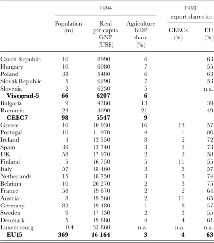
The current front-runners in the eastern enlargement race are the Czech Republic, Hungary, Poland, Slovenia and the Slovak Republic (although human rights issues threaten to disqualify the latter from the race). Even these front-runners, however, are quite different economically from the EU15, as Table 1 shows. For instance, the EU15 are on average half as agricultural and two and a half times richer than the Visegrad-5. The much lower per capita income in the CEECs reflects (by definition) a much lower labour productivity. A good part of this difference is accounted for by the inferior state of eastern capital stocks and technology. Such factors can be changed rapidly, since installing new machines and adopting new technology are relatively simple, given the high level of education in the CEECs. Another part depends upon much more intangible factors, such as a well-functioning public administration, respect and knowledge of commercial law and job-specific training of workers. Since these intangibles are in good shape in some CEECs (e.g., the Czech Republic, Slovenia, Estonia, Hungary, Poland and the Slovak Republic), but in bad shape in others, the CEECs are likely to have very different growth rates in the coming decades. For instance, for the Visegrad-5 and Estonia, the prospects of rapid investment in physical and knowledge capital lead most observers to predict growth rates that are two or three times those of western Europe. This growth gap will narrow income differentials, but it will still take decades before even the richest CEECs catch up to the EU15 average.
Differences between the CEEC and EU populations, multiplied by the income-level differences, imply that the two regions are of very unequal economic size. The Visegrad-5 economies taken together, for instance, amount to only about 5% of the EU15 economy. The relative size is important for a fairly simple reason. Inter-national integration boosts incomes by expanding the set of opportunities facing consumers and firms. Typically, this expansion of opportunity enables consumers and firms to arrange their affairs more efficiently, which results in higher output and
income. East – west integration in Europe will plainly expand the CEECs’ opportunities much more than it will expand those of the EU, so we should expect the integration to have a larger percentage impact on the GDP of the CEECs, even without undertaking any formal estimates.
2.2. Trade
The EU15 sell about $40 billion to the CEECs and buy slightly less from them. This trade covers a broad range of goods and consists mainly of two-way trade in similar products, as Figure 1 shows. With the exceptions of ‘chemicals and rubber and plastic goods’, and capital goods (‘transport equipment’ and ‘other machines and equipment’) where the EU is a net exporter, the EU – CEEC trade is approximately
Table 1. Basic economic facts
1994 1993
export shares to:
Population Real Agriculture
(m) per capita GDP CEECs EU
GNP share (%) (%) (US$) (%) Czech Republic 10 8990 6 63 Hungary 10 6080 7 55 Poland 38 5480 6 63 Slovak Republic 5 6290 7 53 Slovenia 2 6230 5 n.a. Visegrad-5 66 6207 6 Bulgaria 9 4380 13 39 Romania 23 4090 21 49 CEEC7 98 5547 9 Greece 10 10 930 16 13 57 Portugal 10 11 970 4 1 80 Ireland 4 13 550 8 2 72 Spain 39 13 740 3 2 73 UK 58 17 970 2 2 58 Finland 5 16 750 5 11 55 Italy 57 18 460 3 5 57 Netherlands 15 18 750 3 3 74 Belgium 10 20 270 2 3 75 France 58 19 670 2 2 64 Austria 8 19 560 2 11 65 Germany 82 19 480 1 8 57 Sweden 9 17 130 2 3 55 Denmark 5 19 880 4 4 61
Luxembourg 0.4 35 860 n.a. n.a. n.a.
EU15 369 16 164 3 4 63
Sources: Population and real GNP/pop. (PPP estimates 1994 Int’l US$s) World Development Report, 1996, table 1. Agriculture GDP share, World Development Report,
1996, table 12. Trade data from WTO database, using WTO definition of CEECs.
balanced product by product. With this sort of trade structure, reciprocal liberaliz-ation can force sectors to expand in both regions due to improved exploitliberaliz-ation of scale economies. At the same time, the relatively unbalanced nature of trade in capital goods points to the potential for significant enlargement-related restructuring in the CEECs that is heavily biased against capital goods.
The EU15’s trade with the CEECs is distributed in a very disproportionate manner. Germany alone accounts for 42% of EU15 exports to the CEECs, while no other member state accounts for more than 10% of the EU15 total. Austria, Belgium, Finland, France, Italy, the Netherlands and the UK each account for 5% or more of the total. At the other extreme, the exports of Portugal and Ireland to the CEECs account for less than 2% of the EU total.
The last salient point concerns the disparity between the importance of the EU market for CEEC exports and the importance of the CEEC markets for EU exporters. Comparing the last two columns of Table 1, we see that the EU market is critical to CEEC exports, amounting to 50 – 60% of all exports (approximately the importance of the EU market for EU nations themselves). However, the CEEC market is fairly unimportant to the EU exporters, with the CEECs taking in about 4% of EU15 exports (including intra-EU trade). While the welfare gains from trade generally stem from imports rather than exports, national trade policies are typically influenced by mercantilist concerns. It is therefore useful to note that the average EU figure of 4% hides a good deal of dispersion. For Germany, Austria, Greece and
Chemicals, rubber and plastic products Food and agricultural goods
Other primary goods
Iron and steel
Semi-processed goods
Transport equipment
Other machines and equipment
Other manufacturers Textiles, clothing and
footwear EU to CEECs
CEECs to EU 5
0 10 15
Figure 1. EU – CEEC trade, 1993 (US$bn)
Finland the figure is at least double the 4% average, but for Portugal, Ireland, Spain and the UK, the CEEC markets are only half as important as the EU average.
2.3. Protection
The final set of basic facts concerns the level of trade barriers in the CEECs and the EU. Due to the Europe Agreements, the EU has phased out all statutory tariffs on CEEC industrial goods, and the CEECs are in the process of phasing out the same on imports from the EU (Faini and Portes, 1995). Note that duty-free treatment of industrial goods is not really preferential in Europe, since about 80% of EU imports are accorded such status. In other words, zero statutory tariffs merely level the playing field for Europe’s major suppliers. Moreover, zero statutory tariffs do not mean free trade. EU-imposed anti-dumping duties and price-fixing arrangements, meant to avoid such duties, greatly restrict CEEC exports in those areas in which they could expand sales most rapidly – iron and steel in particular. The EU also continues to impose quotas on other so-called sensitive industrial goods, such as textiles, clothing and footwear. CEEC exports of non-industrial goods – especially agricultural goods – have been liberalized only slightly by the EU, and there are no concrete plans to liberalize such trade prior to enlargement.
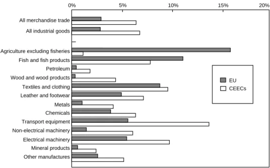
Figure 2 shows the MFN applied tariff rates for the EU and the CEECs for a range of products. There are three main points to be highlighted. First, the CEECs are on average more protectionist than the EU, although both are quite open when
All merchandise trade All industrial goods
Agriculture excluding fisheries Fish and fish products Petroleum Wood and wood products Textiles and clothing Leather and footwear Metals Chemicals Transport equipment Non-electrical machinery Electrical machinery Mineral products Other manufactures EU CEECs 0% 5% 10% 15% 20%
Figure 2. Post-Uruguay Round applied MFN tariff rates
compared to developing countries in Asia, Africa and Latin America: the CEECs’ average applied tariff is 6.5%, while the EU’s is 3%. Second, the CEECs’ average of 6.5% consists of somewhat higher-than-EU rates on industrial goods, but much lower-than-EU rates on agricultural goods. As a result, the enlargement is likely to lead to an important increase in CEEC agricultural protection against third-country suppliers. The same sort of pattern emerged with the Iberian accession, and in that instance third countries, notably the USA, demanded compensation for the hikes in farm protection. The last point is that the gap between the CEEC and EU rates varies widely among industrial goods. For instance, the gap is more than 10% in transport equipment, but less than 2% in textiles and clothing, petroleum and mineral products.
This asymmetry of protection rates has important implications for the welfare effects of enlargement. Since two-thirds of CEEC imports are from the EU, and this trade will become free, the ongoing process of joining the EU implies a great deal of tariff cutting in the CEECs, but very little tariff cutting in the EU (especially since imports from the CEECs amount to only 4% of EU15 imports). Because most gains come from own-liberalization, the initial levels of protection suggest that enlargement will lead to much greater income gains in the CEECs than in the EU. At the same time, like the pattern of trade, the pattern of protection also suggests that negative restructuring in the CEECs will probably be concentrated in heavy industry.
3. MEASURING THE ECONOMIC BENEFITS
The preferential integration of two regions can produce a vast array of economic effects. No longer is it enough to think about ‘trade creation’ and ‘trade diversion’: the last ten years have seen important theoretical advances in this area.1 Since our
results depend heavily on effects that may not be familiar to non-specialists, section 3.1 provides intuition for the new effects and their relationship with older, more standard effects. Section 3.2 briefly presents how we capture all of the various effects of eastern enlargement on the CEEC and EU economies. Section 3.3 discusses the policy experiments and results for the EU as a whole when we make conservative assumptions. Section 3.4 makes less conservative assumptions, while the final section presents some rough calculations on how the gains will be distributed among the incumbent EU15.
3.1. A primer on the theory of preferential trade liberalization
A useful classification divides all effects into allocation or accumulation effects (an alternative, but misleading, dichotomy is static and dynamic effects). Allocation
effects capture the way in which integration induces changes in economic efficiency through resource and expenditure reallocation. Even if we ignore imperfect competition and scale economies (as in the earlier trade creation and diversion literature), we take into account three types of allocation effect, one of which was identified in the last ten years.
The first of these perfect-competition effects stems from trade volume changes: when a good’s domestic price exceeds its border price (i.e., the price paid to foreign suppliers), increasing imports lowers the cost of consuming goods and thus raises national welfare. This is the traditional trade creation effect. Clearly, contracting imports in such cases produces the opposite result.
The second effect stems from changes in trade prices. When a country is a net importer of a good, a drop in the border price is beneficial (domestic producers lose less than domestic consumers gain), while the opposite holds when the country is a net exporter. This corresponds roughly to trade diversion, but it is really a composite of two effects: supply switching (typically from a supplier outside the preferential trade area (PTA) to a PTA-based supplier) and the induced changes in the applicable border prices. For instance, if imports came from the lowest-cost supplier prior to preferential liberalization, any switching from non-PTA suppliers to PTA suppliers tends to raise the border price that PTA members pay after the arrangement is implemented. Deepening a PTA tends to lower welfare for PTA members when supply switching is accompanied by a rise in applicable border prices.
The novel third effect is interesting, since it shows that ‘trade diversion’ (at least the supply-switching part) may actually be welfare improving, although understand-ing this requires a bit of background. The third effect focuses on trade rents: that is, the revenue that may arise from selling across the gap between low border prices and high domestic prices. Textbook import barriers hand the trade rents either to the domestic government (as in the case of tariffs) or to foreigners (as in the case of price-fixing arrangements or voluntary export restraints). Yet textbook trade barriers have to a large extent been eliminated in western Europe: about 80% of western European imports are duty-free and, even including applied dumping duties, the EU’s trade-weighted tariff is only 3%.
European trade is not free, of course, since many ‘frictional’ barriers drive wedges between domestic and border prices by raising the real cost of trade (unharmonized product standards are the prime example). Such barriers create no trade rents, they just burn up resources. The interesting point is that eliminating frictional barriers – even on a preferential basis – unambiguously lowers border prices. Thus we may observe trade diversion (in the sense of supply switching) that raises national welfare by lowering the cost of imports. Consideration of frictional barriers is central to the evaluation of eastern EU enlargement, since the Europe Agreements eliminate most of the textbook import barriers. To put it differently, EU membership will promote the CEECs from members of a free trade agreement to members of the EU’s single market.
Since Krugman (1979), trade economists have highlighted the importance of imperfect competition and scale economies. In the process, three ‘new’ allocation effects have been identified: producer profit effects, scale effects and variety effects (see Francois and Roland-Holst (1996) for details). The first is easy. In sectors where the local price exceeds the average cost of production, an expansion of output raises welfare, since the marginal value of extra output (the price) exceeds the extra cost. A fall in production yields the opposite result. This effect is sometimes called the pure profit effect. Scale effects are also quite intuitive. Average cost falls with the scale of production in most industries, where scale may refer to the size of firms or the size of sectors. Because lower average costs mean more output with the same inputs, positive scale effects tend to improve national welfare. Lastly, integration can increase the range of varieties available to consumers in both regions. More choice makes consumers happier, and, on the production side, a broader variety of input choices can boost industrial productivity.
Accumulation effects are quite a different matter. They highlight channels through which trade arrangements can alter the level of national resources – especially capital stocks – rather than merely reallocate the existing stock of resources. By their nature, accumulation effects tend to have a much larger impact on GDP than allocation effects. Allocation effects involve taking resources out of one activity and putting them into another. The benefit of doing this is limited by the degree to which resource efficiencies initially differ across sectors. In the absence of trade barriers (or other distortions), market forces even out initial sectoral resource efficiencies. It is not surprising, therefore, to find that allocation effects typically yield very small gains in countries that start with well-functioning market economies. Since accumulation effects change the stock of resources, they can lead to much larger changes in the amount of goods that can be produced by the same labour force. (See Baldwin and Francois (1996) and Francois and Reinert (1996) for efforts to capture such effects empirically.)
3.2. The policy experiments and results: modelling eastern enlargement
Given enough data, one could construct and estimate an econometric model of the world economy that allowed for all the allocation and accumulation effects mentioned above. This would clearly be the best approach, were it feasible. Unfortunately, the current state of data and theory precludes this tack. Instead, we simulate the economic effects of eastern enlargement by postulating a number of key relationships.2 As briefly summarized in Table 2, the model covers all world trade
2Technically, we employ a calibrated general equilibrium model. While the simulation approach has its shortcomings,
it is really the only game in town. This conclusion has also been reached in other fields of applied policy analysis. For instance, proposed tax changes are routinely evaluated with calibrated simulation models in the empirical public finance literature.
and production, and it allows for scale economies, imperfect competition and endogenous capital stocks. Box 1 provides more discussion of the technicalities for specialists. Interested readers are referred to the 50-page technical appendix to Francois et al. (1995) for detailed discussion of the theoretical structure of the model.
3.3. Conservative estimates
EU membership for the CEECs will involve a broad gamut of policy changes. The most obvious involve: (1) elimination of tariffs and quantitative restrictions on all EU – CEEC trade, including agriculture trade, and (2) adoption of the EU’s common external tariff (which is generally more liberal than the CEECs’ current tariffs against non-western European imports). It will also, however, grant ‘single market access’ to the EU15 markets for CEEC firms, and the same access for EU firms to the CEEC markets. Single market access involves hundreds of very specific rules (not all of which have even been implemented by the incumbent EU members), so it is impossible to describe in full here. The idea, however, is that it establishes the free movement of goods, services, capital and people. The latter two require open capital markets and unfettered migration. The main elements ensuring the first two freedoms are: (1) the mutual recognition of health, safety, industrial and environmental product standards (after adoption of common minimum standards), (2) the adoption of a common competition policy and a common state-aids policy, and (3) removal of frontier controls.
Incorporating the tariff changes in our model is straightforward, with the exception of agricultural trade. Even though there are no tariffs or quotas on internal EU farm trade (mad cows excepted), the common agricultural policy
Table 2. Sectors and regions in the model
Sectors Regions
Agriculture, forestry, fisheries CEEC7
Primary mining and fuels EU15
Processed foods EFTA3
* Textiles Former Soviet Union
Apparel North American Free Trade Area
* Non-ferrous metals Asia-Pacific
* Iron and steel North Africa and Middle East
* Chemicals, rubber and plastics Sub-Saharan Africa
* Fabricated metal products Rest of world
* Transport equipment
* Other machinery and equipment
Other manufactures Services
* Scale economies and imperfect competition.
Note: CEEC7 = Czech Republic, Slovakia, Poland, Hungary, Slovenia,
Box 1. The simulation model: technical presentation
Our model divides the world into nine regions each with thirteen sectors (see Table 2 for region and sector names). Consumers’ demands for final-good sectors are generated from a representative regional household with Cobb – Douglas preferences over sectoral composites. Each sector consists of differentiated products and consumers’ demand for these are generated by CES preferences. In seven of the sectors (marked by asterisks in the table), we allow for scale economies and imperfect competition, along the lines of the standard Dixit – Stiglitz monopolistic competition model (e.g., fixed mark-ups and free entry). The other sectors are perfect-competition, constant-returns sectors but each region’s output is assumed to be differentiated (Armington assumption).
The central feature of all computable general equilibrium models is the input– output structure that explicitly links industries in a value added chain from primary goods, over continuously higher stages of intermediate processing, to the final assembling of goods and services for consumption. The link between sectors may be direct, like the input of steel in the production of transport equipment, or indirect, via intermediate use in other sectors. The model implements this input – output structure by assuming that firms use a mixture of factors (labour and capital) and intermediate inputs. Specifically, factors are combined according to a CES function, while intermediates are used in fixed proportions. This has two significant ramifications: (1) the price of intermediates enters firms’ cost functions, so price-raising trade barriers directly affect firms’ productivity, and (2) firms’ demand for each variety of intermediates follow standard CES derived-demand functions.
With product differentiation in all sectors (differentiation at the firm level in the increasing-returns sectors and at the regional level in the perfect-competition sectors), the model supports two-way trade in all traded sectors. The cost of trade (a combination of trade and transport services) is modelled explicitly. Revenues from non-frictional trade barriers are returned to the representative consumer in each region.
Regional labour supplies are assumed to be fixed, but regional capital stocks are endogenous. Capital, which includes buildings, is produced according to a fixed-coefficient production function from various intermediate inputs, such as transport equipment and other machinery. The global steady-state capital stocks is the level which balances global savings (regional savings rates are fixed) with global depreciation. Regional capital stocks are then determined by a simplified global capital market. That is, the regional stocks move to maintain the base case relative returns across regions.
The model is calibrated to social accounting data from the last revision (August 1996) to the Global Trade Analysis Project (GTAP) version 3 dataset. The GTAP dataset includes information on national and regional input – output structure, bilateral trade flows, final demand patterns and government intervention, and is benchmarked to 1992. Protection data are based on World Bank and WTO data on pre- and post-Uruguay Round protection. We work with the post-Uruguay Round protection data. Formally, this involves first modelling the impact of the Uruguay Round. We then work with the estimated post-Uruguay Round set of social accounting data for the simulation results presented in this paper.
(CAP) ensures that trade is definitely not free. We capture this by including a very stylized CAP. Subsidy payments to the EU15 farm sectors are assumed to be sufficient to maintain output at pre-enlargement levels. A second, very different difficulty arises in trying to model single market access. The complexity of single market access makes it impossible for us to model it explicitly in a general equilibrium model. The standard solution to this problem is to model single market access crudely as a reduction in the real cost of trade. In our simulations, we quantify this as a 10% reduction in real costs of all CEEC – EU trade.
Our first set of results – what we call the conservative scenario – considers only the allocation and accumulation effects that the above-mentioned policy changes have on the global economy. These are presented below. Section 3.4 presents a less conservative set of policy experiments, which allow eastern enlargement – and implicitly the failure of eastern enlargement – to change the risk premiums on investment in the CEECs.
Table 3 presents the aggregate real income and trade effects of eastern EU enlargement for the conservative scenario.3 Three aspects of the results are worth
mentioning. First, all European regions gain from enlargement. This need not have been the case. For instance, one might have guessed that at least the non-EU European countries (EFTA3 and ex-USSR) might have been harmed by the discriminatory aspects of eastern enlargement. Second, while all income effects are positive, the CEECs gain much more than the EU in relative terms. Specifically, the CEECs’ 1.5% rise in real income is seven times larger than the EU gain. Most of the asymmetric gain can be explained by the fact that the CEEC economies were initially more distorted, so EU enlargement involves a greater degree of own-liberalization. For instance, the initial CEEC applied tariff rate is twice that of the EU. Nevertheless, since the EU15 economy is twenty times larger than that of the
Table 3. Real income effects: conservative case
Real income change Real income change
(1992 ECUbn (% change
change from base case) from base case)
CEEC7 2.5 1.5
EU15 9.8 0.2
EFTA3 0.2 0.1
Ex-USSR 1.1 0.3
Notes: This is a comparative steady-state exercise, so real income changes
are not equivalent to utility-based welfare changes. Real income is GDP. EFTA3 is Norway, Iceland and the Swiss-Liechtenstein customs union.
Source: Authors’ calculations.
3
CEECs, the ECU gain to the EU is almost four times greater than the gain to the CEECs. The third point concerns the aggregate export effects. Due to the combined effect of the CEECs’ own-liberalization, improved access to the EU market, and the expansion of the CEEC economies due to positive accumulation effects, the CEECs are projected to increase exports by more than 25%. Since enlargement is only a mild liberalization for the incumbent EU members, aggregate EU15 exports rise by only 1.5%.
As far as the impact on the EU is concerned (by far the most sensitive issue, given EU leaders’ fears about the economics of enlargement), our results are in line with Brown et al. (1995). Those authors find that a free trade area between the Visegrad countries and the EU would raise EU real income by ECU13.3 billion. Our results are not exactly comparable to the Brown et al. findings, however, since those authors undertake an exercise that differs in two important ways (apart from the obvious fact that they use a different CGE model that is calibrated to a different data set). First, they examine the effects of a free trade area, not a customs union. Consequently, they do not require the CEECs to adopt the EU’s common external tariff. This potentially makes an important difference, since the CEECs have much higher tariffs on heavy industry and much lower tariffs on food. As a result, our results incorporate the effects of much more substantial industrial restructuring than do theirs. Second, they consider only the Visegrad countries rather than the CEEC7 as in our exercise. The economic impact they find for the Visegrad countries amounts to about ECU9 billion, which is much larger than our conservative estimates. As we see below, however, the ECU9 billion of Brown et al. is much smaller than the number we find in our ‘less conservative’ scenario, to which we turn now.
3.4. Less conservative estimates
3.4.1. The risk premium effect. The conservative scenario discussed above
includes a simple variation on the classical savings mechanism, by which increased returns to regional capital lead to increased levels of regional investment and hence to an increased capital stock. We do not believe, however, that this will be the end of the story. The CEECs are currently a risky place to invest. Fortunes have been made by those who are lucky (or well connected), but fortunes have been lost. The uncertainty stems from microeconomic sources and macroeconomic sources. Since the transitions began, the micro sources have included, inter alia, bank failures, privatization, bankruptcies, unpredictable changes in subsidy, trade and indirect tax policies, and sudden changes in the legal system, industrial standards and regulation, and administrative procedures. In short, these are economies in transition. At least in those CEECs that seem likely to join the EU soon, the prospect of EU membership has already greatly reduced the riskiness in one very direct way. EU membership gives investors some idea of the direction in which transition is
heading. Such is not the case for other economies in transition – the examples of Russia and the Ukraine come to mind – that have virtually no prospect of joining the EU.
The macro sources of uncertainty include unanticipated changes in inflation rates, interest rates and exchange rates. In many of the CEECs, these macro sources of instability are linked to the micro sources. One classic link is that attempts to subsidize sunset industries on a large scale lead to large fiscal deficits that are covered by printing money. Also, a large measure of the inflation in these countries stems from initial price shocks that occurred when prices were liberalized and currencies deeply devalued. Finally, given the potential for political instability in Russia and the lack of security guarantees from, for example, NATO, there remains some small uncertainty about the territorial integrity of the CEECs, especially prior to EU membership.
Joining the EU will make the CEECs substantially less risky from the point of view of domestic and foreign investors. On the micro side, EU membership greatly constrains arbitrary trade and indirect tax policy changes. It also locks in well-defined property rights and codifies competition policy and state-aids policy. By securing convertibility, open capital markets and rights of establishment, member-ship assures investors that they can put in and take out money. Finally, EU membership guarantees that CEEC-produced products have unparalleled access to the EU15 markets (which account for almost 30% of world income). On the macro side, membership puts the CEECs on a path to eventual monetary union and thus provides a solid hedge against inflation spurts. These two aspects of membership are likely to have a related impact on investor confidence and are likely to be mutually reinforcing.
3.4.2. Guesstimating the impact on the CEEC risk premium. The statement
that EU membership will make the CEECs less risky sites for physical investments seems uncontroversial to us. The hard and therefore controversial part is to quantify the impact that enlargement will have on CEEC risk premiums. Rates of return on capital differ sharply across nations, and these differences are often very persistent. One common explanation for this is that investors demand a risk premium on funds invested in nations with economic and/or political environments that are perceived as unstable.
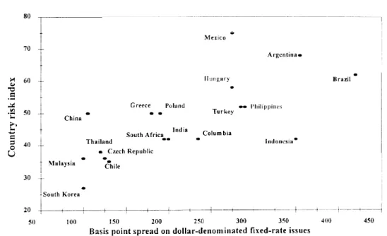
As Figure 3 shows, country risk does correlate with rates of return. The figure plots, on the horizontal axis, World Bank estimates of the basis point spread charged to emerging economies for dollar-denominated fixed rate issues in 1994. The vertical axis plots country risk indexes for 1995. (A similar pattern, not shown, holds for the spread on the effective dollar yield of domestic debt issues calculated from IMF International Financial Statistics data for medium-term domestic debt issues adjusted for currency movements.) The Czech Republic, Poland and Hungary are arrayed along the middle of the spectrum, with the Czech Republic ranked as the
best risk and Hungary as the worst. Poland is ranked as a risk comparable to Greece. Russia is off the charts on both axes, and data for Bulgaria and Romania are unavailable (not a good omen). The unweighted CEEC average for those in the sample (not shown) is located quite close to Poland.
This pattern suggests a simple, albeit rudimentary, way of quantifying the impact of risk on national capital markets. We make the somewhat ad hoc assumption that the CEEC average country risk index moves down to the range of Portugal after EU accession. This implies that the relative return demanded by savers for investment in the region should drop by roughly 15%, which translates to about 45 basis points. Finally, we retain the same trade barrier changes as in the conservative scenario and we assume that the relative regional rates of return are the same for all regions except the CEECs (which are lowered by 45 basis points). Of course, the CEEC capital stock must rise substantially to bring CEEC capital’s actual rate of return down to the new assumed steady-state level.
This approach is plainly quite ad hoc, but we feel that it captures an element in the EU membership that is essential for the CEECs. Moreover, there is some historical evidence suggesting a correlation between investment and membership, at least in poor entrants. First, we note that a range of case studies for the Iberian countries also support our basic contention that EU membership can be good for investment in poor entrants. For Spain, the boost to investment from accession and the effect on the current account are documented by ViÓnals et al. (1990) and by Ortega et al. (1990). The stimulus to foreign investment is analysed by Bajo and Sosvilla (1990).
Figure 3. Risk and return in emerging markets
Sources: Horizontal axis risk premium: World Bank estimates from 1996 World Debt Tables, Extracts.
For both Portugal and Spain, Braga de Macedo and Torres (1990) specifically demonstrate the decline in country risk premium following accession.
3.4.3. Prima facie historical case. In addition to the detailed case studies listed
above, we can make a prima facie case by eyeballing historical data for the six countries that joined the EU during the 1973, 1981 and 1986 enlargements (the 1995 enlargement is too recent to permit study). However, to interpret the historical evidence correctly requires a little theory. A country’s capital stock is fixed by the equality of the demand for capital and the supply of capital. Anything that shifts either schedule will change the equilibrium (i.e., steady-state) capital stock. If the change requires the nation’s capital stock to rise, above-normal investment will result. The opposite is predicted for changes that require the nation’s capital stock to drop.
The theoretical situation is shown in Figure 4, where the solid lines indicate the initial situation. The demand curve shows that the marginal product of capital declines when the capital stock rises, due to economy-wide diminishing returns. The capital supply curve shows that savers will demand higher rates of return to invest more in the particular country, reflecting both the willingness of consumers to postpone consumption by investing today and a portfolio analysis for savers. The initial equilibrium capital stock, shown as K0, is not at the intersection of the supply
and demand curves for capital, since we assume that the country faces a risk premium. On average, investors earn r0 on their investments, but due to the
uncertainty involved, they act as if earning an expected return of r0 with uncertainty
were equivalent to earning r0− d0 with certainty (here d0 is the country’s risk
premium).
Joining the European Union can affect the position of the demand curve and it can affect the size of the risk premium. The demand shift can come from many mechanisms. For instance, membership improves the country’s market access to Europe’s largest markets. If the country exports goods (e.g., manufactured goods)
that are capital intensive relative to its non-traded goods (e.g., government services) then extra market access shifts up the nation’s capital demand curve. This shift is illustrated in the diagram by a dashed line. (See Baldwin and Seghezza (1996) for a formal illustration of this trade-and-growth link and for many others.) The reduction in the risk premium can come from many sources, including a change in the underlying uncertainty (i.e., a bona fide stability of the economy) and an enhanced ability of investors to diversify risk (i.e., when domestic residents get improved access to wider capital markets). The post-enlargement risk premium, shown as d, in the figure, is less than the pre-enlargement premium of d0.
These two changes – a drop in the risk premium and an upward shift in the capital demand curve – result in an unambiguous increase in the capital stock (from K0 to K, ), but an ambiguous effect on the real rate of return. To see this, note that
as we have drawn it, the real return rises from r0 to r,, but if we had eliminated the
risk premium altogether, we would have predicted a drop from r0 to the point
where the new demand and old supply curves intersect.
There are a few other things to note. First, the upward demand shift will normally be associated with an increase in the profitability of existing capital. This should show up in the average behaviour of the stock market, as long as the stock market reflects a broad sample of firms. The caveat comes from the fact that liberalization almost always harms some firms and sectors, even when it is beneficial to the nation as a whole. If the stock market is dominated by, say, state-controlled white elephants that will face increased pressure in a more liberal economy, then enlargement may be accompanied by a drop in the stock market index. Second, the diagram does not distinguish between domestic and foreign investors. An improvement in the national investment climate should attract more investment from both sources. This is likely to leave three kinds of ‘footprint’ in the data. The investment-to-GDP ratio should rise, the current account should deteriorate as more foreign funds come in, and the net direct investment figures should improve. Finally, note that all of these initial effects eventually wear off as the capital stock adjusts to its new level.
3.4.4. Historical data. We turn now to the evidence for the six countries that joined
the EU during the 1973, 1981 and 1986 enlargements. Figure 5 shows the current account deficits for the 1973 entrants (Denmark, Ireland and the UK), the 1981 entrant (Greece) and the 1986 entrants (Portugal and Spain). For the six, entry was generally accompanied by an increase in capital inflows, although the pattern is certainly not stark. For instance, when we calculate the mean current account deficit for each entrant during the five years preceding accession, and the mean for the year of accession plus five years, we see that in all cases except Portugal the post-accession capital inflow is larger.
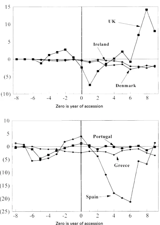
Figure 6 shows the change in stock market indices for the six entrants. The Iberian enlargement was clearly accompanied by a stock market boom, while the Greek accession did not produce such a result. The evidence for the 1973
Figure 5. Current accounts for 1973, 1981 and 1986 entrants (8 years pre- and 9 years post-accession where data permit)
Source: IMF IFS databank.
Zero is year of accession Zero is year of accession
enlargement is much more confused – at least in part due to the unsettled macroeconomic environment of the early 1970s (the first oil price shock and rising inflation). To provide a benchmark, we also plot the GDP-weighted average movement of the EC5 stock markets (the EC6 less Luxembourg, for which data are available only from 1970). We see that the three entrants (Denmark, Ireland and the UK) did no better than average for the first few years. Further out, however, say nine years after membership, Ireland is doing much better than the average of incumbents. This fits in with our general idea that enlargement is likely to have the greatest impact on the countries that are economically the furthest behind the EU incumbents: namely, Ireland, Greece, Portugal and Spain. When it comes to stock market data, Greece is the exception among the poor entrants. As we shall see, the poor performance of Greece is echoed in several other indicators. To us this indicates that EU membership provides an opportunity for poor countries to catch up. There is, however, nothing automatic about the benefits.
The real interest data are much harder to interpret. As our theoretical discussion indicated, the combination of increased demand and reduced risk premium can result in either an increase or a decrease in real rates. Moreover, inspection of the data shows examples of both, so we do not provide a plot of the data. In brief, we find that the Iberians seem to have experienced a rise in real rates, but the pattern is much less clear for the other four nations.
Finally, Figure 7 shows the investment-to-GDP ratios (gross fixed business investment as a share of GDP) for all six entrants. Until the mid-1970s, Portugal and Spain were under dictatorships that typically ruled the economies with a heavy and sometimes arbitrary hand. Investment in these countries was consequently a risky business for those without close connections to the dictators. The end of the Iberian
Ireland Portugal UK Spain EC5 Denmark Greece 400 300 200 100 0 5 4 3 2 1 0 1 2 3 4 5 6 7 8 9
Zero is year of accession
dictatorships and their EU membership bids transformed the investment climate on the Iberian peninsula. As the figure shows, the change in the Portuguese investment rate is especially marked around the beginning of accession talks in 1978. The talks dragged on, however, proving much more difficult than foreseen. The final outcome was not clear (at least for Spain) until 1984 – 5. The accession treaties were finally signed in 1985, with entry occurring in 1986. It is interesting to note that the investment rates in Portugal move in tandem with progress in the membership talks. Spain’s investment rate did not pick up until membership was virtually assured. Recent years have seen the Iberian investment rates converging towards the EU averages. It seems, therefore, that the investment boost was transitional. The figure shows that Ireland experienced a similar investment boom during the decade following its accession. For Greece, however, accession had little impact on investment.
Clearly this evidence does not prove that EU membership is good for investment. Nor does it justify our specific quantitative assumption for the effect of accession on country risk. It does, however, provide a prima facie case that EU accession can be helpful in encouraging investment in poor entrants (namely Spain, Portugal and Ireland) and support for the assertion that the Iberian investment-led growth in the 1980s was greatly boosted by the prospect of EU membership. An important caveat is that EU membership in the mid-1980s involved far fewer constraints on domestic policy than it does now. Neither the single market programme nor monetary union were faits accomplis at that point.
Ireland Portugal UK Spain EC5 Denmark Greece 180 160 140 120 100 80 60 40 5 4 3 2 1 0 1 2 3 4 5 6 7 8 9 10
Zero is accession year
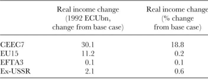
3.4.5. Simulation results. Table 4 presents the aggregate impact of enlargement
under the less conservative scenario. Note first that the impact on the EU15 is almost unchanged from the conservative case – under both scenarios, the EU15 gain about ECU10 billion. The same holds true for the EFTA3 and the ex-USSR. The big change is the gain for the CEECs themselves. This should not be a surprising result, since the assumed risk premium reduction impacts primarily on the CEECs’ capital stock. The projected gain – about ECU30 billion – is enormous by the standards of similar simulation models. Most of the extra real income gain comes from the estimated 68% rise in the CEEC capital stock (the CEEC capital stock rises by only 1.2% in the conservative scenario).
Sensitivity analyses of the less conservative scenario are shown in Table 5. The two most arbitrary assumptions in the less conservative scenario are the trade cost reduction and the size of the risk premium reduction. First, still assuming that membership lowers east – west trading cost by 10%, we consider different shocks to the risk premium on central European investment ranging from 0% (this is equivalent to the conservative scenario) to 15% (the less conservative scenario). The first column in Table 5 (top panel) shows that the real income gain of the CEECs falls from ECU30.1 billion to 6.2 billion as the risk premium reduction goes from 15% to 5%. The second column of the top panel shows that the consequences for the EU15 are much less. Second, we hold the risk premium shock at the less conservative scenario assumption of 15% and vary the trade cost reduction assumption. The results for both the EU15 and the CEEC7 (shown in the bottom panel of the table) are little affected by these changes.
That the effects on the CEECs remain large under different scenarios is important. The CEECs are already keen on joining the European Union for geopolitical reasons, so even the finding of a significant negative economic impact would be unlikely to affect their ardour for rapid membership. The same cannot be said for the EU15 and it is the EU15 who will decide the timing of enlargement. True, the EU15 are all committed to admitting the CEECs eventually, but their perception of the large economic costs of eastern enlargement seems to have made them reluctant to hasten the enlargement process.
Table 4. Real income effects: less conservative case Real income change Real income change
(1992 ECUbn, (% change
change from base case) from base case)
CEEC7 30.1 18.8
EU15 11.2 0.2
EFTA3 0.1 0.1
Ex-USSR 2.1 0.6
Notes: This is a comparative steady-state exercise, so real income
changes are not equivalent to utility-based welfare changes. EFTA3 is Norway, Iceland and the Swiss-Liechtenstein customs union.
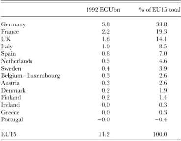
3.5. Sharing out the economic benefits
Our simulation model does not contain individual member states, so we cannot determine how the aggregate gain is distributed among the various EU15 nations. This is, nonetheless, an important political issue, so we present some back-of-theenvelope calculations. Under both scenarios, the simulation breaks down changes in the EU15’s GDP by sector. As a first step, we distribute these sectoral changes to member states using the importance of each member state’s sector (as measured by value added) in the EU15 sector totals. These changes do not add up to the EU15’s aggregate real income gain, since consumers also gain from price changes. The difference – which is due to projected price changes in the enlarged EU – is allocated among incumbent member states according to their share of EU15 income. The results of this admittedly rudimentary procedure are listed in Table 6.4 (The shares are very similar under the two scenarios, so we report only
the estimated distribution for our preferred scenario – the less conservative estimates.)
The gains are distributed in a very uneven fashion. The shares of Germany, France and the UK sum to more than two-thirds of the whole ECU11.2 billion that the EU15 are projected to gain. Given Germany’s overall size and dominance of the EU sectors that are projected to expand the most (transport equipment and capital goods), it is not surprising that Germany gets a third of the total. Both France and
4
An alternative set of calculations, based on the approximation of member state welfare effects through simple partial equilibrium estimates based on member country trade effects, leads to the same qualitative pattern of results.
Table 5. Sensitivity analysis: real income effects (1992 ECUbn change from base case)
CEEC7 EU15
Different risk premium shocks
0% reduction 2.5 9.8
5% reduction 6.2 10.0
10% reduction 14.5 10.3
15% reduction 30.1 11.2
Trade cost reductions (with 15% risk premium reduction)
5% reduction 29.5 10.2
10% reduction 30.1 11.2
15% reduction 30.4 11.8
Notes: These are a comparative steady-state exercise, so real income
changes are not equivalent to utility-based welfare changes. EFTA3 is Norway, Iceland and the Swiss-Liechtenstein customs union.
Table 6. Distribution of gains among EU incumbents (change from base case, less conservative scenario)
1992 ECUbn % of EU15 total
Germany 3.8 33.8 France 2.2 19.3 UK 1.6 14.1 Italy 1.0 8.5 Spain 0.8 7.0 Netherlands 0.5 4.6 Sweden 0.4 3.9 Belgium – Luxembourg 0.3 2.6 Austria 0.3 2.6 Denmark 0.2 1.9 Finland 0.2 1.4 Ireland 0.0 0.3 Greece 0.0 0.3 Portugal −0.0 −0.4 EU15 11.2 100.0
Note: See text for methodology. Source: Authors’ calculations.
the UK get double-digit shares (19% and 14% respectively) – again not surprising, given the size and sectoral composition of the French and UK economies. The Netherlands and Spain each take between about 5% and 10% of the total gain. The Dutch figure comes largely from the fact that this economy focuses on sectors whose GDPs rise with enlargement. The high Spanish figure stems partly from the sharing out of the sectoral GDP gains (the Spanish economy is quite diversified) and partly from the fact that the fairly large size of the Spanish economy ensures that Spain takes a healthy slice of the consumer gains stemming from lower prices. Each of the other incumbents gets less than 5% of the total gain. Portugal is the only incumbent that is estimated to lose on these narrow economic grounds. This loss reflects Portugal’s heavy reliance on textiles (this is the EU sector that takes the biggest hit from enlargement according to our projections). Portugal’s loss, however, is vanishingly small and, given the inherent imprecision of CGE models, it is best to think of this figure as zero.
4. THE BUDGET COST OF A VISEGRAD ENLARGEMENT IN 2000
Since Baldwin et al. (1992) and Baldwin (1994), the costs to the EU budget have acquired a disproportionate prominence in the public debate on eastern enlarge-ment. Yet they are important politically, and some extreme estimates have aroused political reaction. This section quantifies the budget burden by reviewing and evaluating an extensive literature on this issue. It also makes a novel contribution by
using a ‘power politics’ approach to estimating the budget impact. Before turning to the estimates, we present the essentials of the EU’s budget.5
4.1. The EU budget: a primer
Table 7 shows that two items dominate the spending side of the EU budget, the common agricultural policy (CAP) and structural spending (the Structural Funds and the Cohesion Fund). Together these account for over 80% of all EU spending. The importance of structural and agriculture spending accurately reflects their importance in the Union. Dr Pangloss would say this spending helps various regions and groups adjust to the pressures of European economic integration. Machiavelli would say these funds are payoffs to politically powerful special interest groups that might otherwise oppose European integration. Both would agree that these programmes are a key ingredient in the political cement that binds member states into a union and allows the EU to be much more than a free trade area. Eastern enlargement will greatly increase the EU’s economic diversity and thereby multiply the centrifugal forces. Structural and farm spending will continue to be needed to contain them.
Revenue is generated from four main sources. The most important is VAT receipts. According to agreed rules, the Union gets a slice of each member’s national VAT revenue. (The precise rules are very complex; see Strasser (1992) for details.) The second and third sources, namely tariff revenue and agricultural levies (variable tariffs until recently), are quite straightforward: all tariff revenue accrues directly to the EU. The fourth major income source is based on members’ GNPs and is used to ‘top up’ revenue to balance accounts (the budget must be balanced each year). The net effect of these four sources is a modestly progressive tax rate.
Table 7. EU budget, 1994
Revenue Spending
VAT 48.4% CAP 49.4%
Tariffs 18.4% Structural Funds 31.9%
Agricultural levies 3.3% R & D 4.4%
GNP based 27.4% Administration 5.3%
Other 2.1% Foreign aid 6.7%
Other 2.3%
Total (ECUbn) 68.6 Total (ECUbn) 67.6
Source: EU Court of Auditors (1995).
5See El-Agraa (1994) and EU Court of Auditors (1995) for more details. See Laffan and Shackleton (1996) for an
excellent general discussion of the budget, budget politics and a history of the EU budget conflicts that followed previous enlargements.
4.1.1. Structural Funds. The Structural Funds are large transfers to the
disadvan-taged member states and regions. The funds are explicitly aimed at encouraging convergence of per capita income levels. Spending is classified by the nature of the problem it is aimed at. The regions or groups that are the focus of these aims are called Objectives 1 – 6. The most important of these – Objective 1 – accounts for two-thirds of all structural spending.6 Also important is the Cohesion Fund for
countries with national income per capita less than 90% of the EU average; in practice this rule was set to ensure that only the poor-4 (Greece, Ireland, Portugal and Spain) qualified. Structural Funds spending is by far the most rapidly growing budget item since 1988. When the current budget plan ends in 1999, this spending should amount to ECU33 billion – a fourfold increase from 1988. Given that CEEC per capita incomes are all below that of the poorest of the EU15 (Greece), the most relevant aspect of this expenditure is its close link with per capita incomes.
4.1.2. Common agricultural policy. The CAP is a very complicated, expensive
set of policies aimed at raising income and output of the EU farm sector. This support takes two main forms: (1) price floors (every six months agriculture ministers gather to set the ‘correct’ prices for farm products) and (2) direct payments (‘compensation’) to farmers. The direct payments are linked to the price floors, in the sense that they were intended to buy off opposition to the 1992 MacSharry reforms that brought the price floors down towards market-clearing levels. Compensation payments are linked to historical production on land that is taken out of production.
The price floors are maintained with two types of policy: protection and market intervention. Protection is insufficient, since the EU price floors are above the zero-import level. Consequently, the EU must buy up the food shunned by EU consumers at these above-market-clearing prices. This ‘excess’ food is disposed of in one of three ways. It is stored until it rots; it is dumped on the EU market (e.g., the EU subsidizes wheat purchases by EU bakeries); or it is dumped (i.e., sold below cost) on world markets. The rising costs of this ‘intervention’ led to the introduction of production quotas in some products. Since 1984 the food surplus is restricted by quotas per farm (e.g., for milk), and by requiring farmers not to grow food on part of their land. More than half the cost of this support is paid for directly by consumers via the ‘hidden tax’ of protectionism, according to OECD (1992). The
6‘Objective 1’ regions are defined as regions with per capita incomes that are less than 75% of the EU average, and
over 20% of the current EU population is eligible under this objective. This spending is aimed at improving infrastructure and local training. ‘Objective 2’ regions are those that suffer from a decline of traditional industries such as coal and steel. Over 45 million of the EU’s 340 million citizens live in these regions. The spending under this objective is aimed at creating jobs, improving the environment, developing R & D and renovating land and buildings. ‘Objective 5b’ regions are rural areas, like the Highlands of Scotland, that are too rich for Objective 1 but still face development difficulties. The other objectives are aimed at the long-term unemployed (Objective 3), unemployed youth (Objective 4); backward farms (Objective 5a), the eastern states of Germany (Regulation No. 3575/90) and Arctic regions (Objective 6).
rest is paid for out of the EU budget – more precisely, from the European Agriculture Guidance and Guarantee Fund (EAGGF).
The budget costs are mostly linked to food surpluses (output less consumption). The consumption side is straightforward, since food demand varies with income and prices in a predictable manner. The output side is essentially intractable: the hard part is to guess how much CEEC farm yields would rise under the CAP, which depends on the extent to which guaranteed prices and sales would stimulate technology transfers and foreign direct investment by western agro-corporations.
4.2. A survey of existing estimates
There is an extensive literature on the cost of eastern enlargement. Three Cs – CAP, cohesion and contributions – dominate the calculations. Of the three, the level of the CEECs’ national contributions as members is least controversial. All member states put in about 1% of GDP. The big debates are over CAP and cohesion spending. We turn first to the studies on cohesion spending.
4.2.1. Cohesion cash. The best-known early estimation (Courchene et al., 1993) was
based on a simple extrapolation of the current level of per capita Structural Funds (SF) receipts in the two poorest incumbents. While per capita SF receipts vary widely among member states (see Table 8), Courchene et al. (1993) settled on a rounded-off average of Greek and Portuguese receipts: namely, ECU200 per person. The Edinburgh summit promised to double this by 1999, so the figure of ECU400
Table 8. Structural Funds allocation, 1993
Total SF Per capita SF SF as % of
(ECUbn) (ECU) GNP Ireland 1088 311 2.8 Portugal 2327 233 2.6 Greece 1897 184 2.5 Spain 2971 76 0.7 Italy 3398 59 0.4 France 1682 30 0.2 UK 1213 21 0.1 Luxembourg 14 43 0.1 Denmark 107 21 0.1 Belgium 187 19 0.1 Netherlands 206 14 0.1 Germany 870 11 0.1 EU12 15962 47 Portugal and Greece average 208 Poor-4 average 7788 132
Note: Structural Funds (SF) include EAGGF, Regional and Social Funds. Source: Court of Auditors, Report on 1993. GNP/pop. from World Bank.
per person was used to project enlargement costs. Just for the 64 million people in the Visegrad-4 countries, this amounts to ECU26 billion.
This widely influential estimate has been questioned by the European Commis-sion in its Interim Report on eastern enlargement (1995a), and by independent analysts (e.g., Grabbe and Hughes, 1996). The primary criticism points out that ECU400 per capita implies unrealistically high levels of aid absorption for the CEECs. Moreover, CEEC governments under severe fiscal pressure would be unable to provide ‘matching funds’ on anything like the scale that current regulations would require. As Table 9 shows, even with their current low income levels boosted by sustained 5% growth, ECU400 per person would amount to 10 – 15% of these countries’ GNPs in 2000. Suppose we take 5% of GNP as a more realistic upper bound. The projected Visegrad SF spending under this rule amounts to ECU12.8 billion.
4.2.2. How to spend the money. Current incumbents are having trouble spending
all the SF allocated to them: in 1994 actual expenditures were only 70% of the planned expenditures, partly because of the ‘matching funds’ constraint. Yet the structural problems facing the transition economies dwarf those of Greece and Portugal. One can easily think of ways of spending cash productively on the CEECs. For example, the human capital infrastructure needs updating. Expensive training courses in western Europe and consultancy fees for western experts could rapidly soak up ECU400 per person per year. The environmental infrastructure could also devour large amounts. Lastly, one might argue that the CEECs should be exempted from making national contributions. To put numbers to this, say Poland managed to spend as much as Ireland on traditional Objective 1 projects (2.8% of GNP) and was exempted from national contributions (1% of GNP). Per Pole, this would account for ECU74 in Objective 1 aid and ECU27 in exempted contributions. Next suppose Poland sent 0.5% of its population on training courses in western Europe and paid western consultancies to train another 0.5% of its population in-country. Taking the
Table 9. Projected Structural Funds spending
Projection assuming Implied aid Projection assuming
ECU400 per capita absorption 5% of GDP
(ECUbn) (%) in 2000 (ECUbn) Czech Republic 4.1 9.3 2.2 Slovak Republic 2.1 13.3 0.8 Hungary 4.1 7.8 2.7 Poland 15.4 12.4 6.2 Slovenia 0.8 4.2 0.9 Visegrad total 26.6 12.8
EU’s HCM grants in the early 1990s as a landmark (i.e., ECU40 000 per year per participant) for this training, we get to an average of ECU400 per Pole for training. All this is without considering spending on environmental clean-up. Moreover, as section 4.3 shows, the EU has been willing to change spending rules for new entrants. Adding in new poor countries will lower the EU average income. Recalling that Objective 1 status (this status qualifies the region for big transfers) requires a region to be below 75% of the EU average, we see that enlargement will necessarily lift some currently eligible regions over the 75% line! While politics makes this unlikely, the possibility does suggest a source of savings on SF spending. Begg (1996) calculates that an aggregate population of 45 million would lose their Objective 1 standing if the ten CEECs were admitted. Spain would also lose its Cohesion Fund status. We do not attempt to calculate these savings because we believe that the rules will probably be changed to maintain the incumbent regions’ Objective 1 status. All in all, therefore, it seems that a 5% of GNP limit is the most reasonable estimate. Ireland, Greece and Portugal have very different per capita income levels, yet each of them receives approximately 2.5% of its GNP in SF. Doubling that rate, we take the implied ECU13 billion for the Visegrad-4 as the consensus estimate.
4.2.3. CAP cash. The debate on the cost of extending the CAP to the Visegrad-4 is
far more complex, due to the complexity of the CAP itself, the lack of accurate data on CEEC farms, and the rapidly evolving nature of eastern agriculture. The range of estimates is correspondingly wide. Table 10 shows estimates for the CAP cost of a Visegrad enlargement that range from ECU4 billion (Brenton and Gros, 1993) to ECU37 billion (Anderson and Tyers, 1993). The more recent estimates, however, have converged significantly. There are two main reasons for this. First, much better data became available with Jackson and Swinnen (1994). Second, the impact of the MacSharry reforms was much clearer after a few years of implementation. For these reasons, all 1995 and 1996 estimates put the cost at ECU5 – 15 billion with ECU10 billion being a fairly representative estimate.7
Tangermann (1996) points out that two key elements lead to the wide range of estimates. First is the assumption concerning eastern farm productivity. The CEEC farm sectors, like every other sector, experienced a sharp decline in output during the early transition years (however, industrial output fell even more quickly than farm output). The reasons were abnormal climatic conditions in 1992 and 1993, a sharp drop in real output prices accompanied by a sharp rise in input prices, and disruption of marketing infrastructure (see EC, 1995b). The low-end estimates essentially assume that this drop is permanent and would not be reversed by the 40 – 50% price rises that would come with the CAP. The high-end estimates assume
7
Despite the wide range of numerical estimates, virtually all independent authors agree on a key qualitative conclusion: the CAP must be reformed before the eastern enlargement.
that massive technological transfers and/or direct investment by western agro-industry would raise eastern yields to western levels. The second factor is assump-tions about CAP reform. The earliest estimates ignored the MacSharry reforms, especially supply controls, set-asides and compensation payments.
CAP costs face two external limitations, neither completely immutable, but both politically difficult to alter. The first is the EU’s own cap on CAP spending increases. An EU rule – in effect since 1988 – limits CAP spending to rise not faster than 74% of the Union’s GDP growth. If this rule, which was respected during the last enlargement, were applied to a Visegrad enlargement in 2000, CAP spending could rise by no more than about ECU0.9 billion.8 Plainly this rule will be binding. The
second involves the GATT commitments undertaken by the CEECs during the Uruguay Round. Most CEECs bound their protection rates and subsidized export levels far more stringently than did the EU. Thus, according to Tangermann (1996), even the conservative estimates suggest that the Visegrad-4 would violate their GATT cereals export commitments by 400 – 500% under the CAP. Of course, Article 24 of GATT would in principle allow the CEECs to break these commit-ments when they join the EU’s customs union, but non-European farm exporters will demand compensation. For instance, the EU awarded compensation to the US farm interests following the 1986 and 1995 enlargements.
4.2.4. How reasonable are the estimates? There is a simple test of the
reasonableness of the CAP estimates. Table 11 shows the CAP cash per farmer and per hectare in the EU12 in 1994. Countries are ranked in descending order of average receipts per farmer, from Belgium’s spectacular 12 300 to Portugal’s modest
Table 10. Estimated CAP cost of eastern enlargement (ECUbn)
Study Visegrad-4 CEEC10
Anderson and Tyers (1995) 37
Tyers (1994) 34
Brenton and Gros (1993) 4 – 31 32 – 55
MahÑe (1995) 6 – 16
Tangermann and Josling (1994) 9 – 14
EC (1995c) 12
Slater and Atkinson (1995) 5 – 15 9 – 23
Tangermann (1996) 13 – 15
Note: Slovenia joined the Visegrad-4 after the studies were completed. Sources: See References.
8Using the Commission’s Interim Report statistics on Visegrad and EU15 GDPs, and assuming 5% and 2% growth
for the Visegrad-4 and EU15 respectively, the Visegrad enlargement would increase EU GDP by only 3%, so CAP spending can rise by only 2.22%. The current Financial Perspective foresees CAP expenditures of ECU38.4 billion.