Random walk and gap plots of DNA sequences

CABIOS

Random walk and gap plots of DNA sequences

P.M.Leong and S.Morgenthaler

Abstract

Genomic sequence analysis is usually performed with the help of specialized software packages written for molecular biologists. The scope of such pre-programmed techniques is quite limited. Because DNA sequences contain a large amount of information, analysis of such sequences without underlying assumptions may provide additional insights. The present article proposes two new graphical representa-tions as examples of such methods. The random walk plot is designed to show the base composition in a compact form, whereas the gap plot visualizes positional correlations. The random walk plot represents the DNA sequence as a curve, a random walk, in a plane. The four possible moves, left/right and up/down, are used to encode the four possible bases. Gap plots provide a tool to exhibit various features in a sequence. They visualize the periodic patterns within a sequence, both with regard to a single type of base or between two types of bases. Introduction

Statistical analyses of nucleic acid sequences have been carried out to answer questions about (i) frequencies of the occurrence of subsequences (words), (ii) similarity with known sequences stored in data banks, (iii) biological functions encoded in DNA, (iv) evolution, (v) taxonomy, etc. Such analyses typically include several types of plots as well as numerical summaries to identify similarities within or across sequences, to count frequencies of words or to fit models. Many ideas, techniques and algorithms are discussed in the books by Sankoffand Kruskal (1983), Doolittle (1990) and Gribskov and Devereux (1991) which contain also an extensive bibliography.

During the last few years the literature on mathematical and statistical methods in the analysis of DNA data has increased at a fast pace. The probabilities of various structures of sequences have been calculated under the assumption of complete randomness or using more sophisticated Markovian hypotheses. These results can be used to assess the statistical significance of patterns Nestle Research Centre, Vers-chez-les-Blancs, 1000 Lausanne 26 and 1 Ecole Polytechnique Federate, Departemenl de Mathematiques, 1015 Lausanne, Switzerland

2 To whom correspondence should be addressed. E-mail. morgi@masg26. epfl.ch

observed in a particular sequence. While this is an important aspect, the relation between statistical signifi-cance and genetic meaningfulness remains unclear. Some patterns found to be remarkable from a statistical view point, may well turn out to have no biological interest. And more importantly, patterns that seem quite weak and explainable as chance happenings, might turn out to be of great genetic significance. There is a need for many more methods that guide the geneticist in his learning about a given DNA sequence. Methods that might provide help in spotting an anomaly, without presupposing what the anomaly might be. As long as a sequence analysis is not narrowly focused, graphical representations of sequences will play an important role.

Plots are useful on three different levels. First, they are often the best way to communicate the result of an analysis, even if the analysis is of a numerical nature. Plots can also help in checking for the presence of an effect. Charts of this type are designed with a particular objective in mind and make use of the human eye rather than a computer algorithm. Last, but certainly not least, plots are the primary tool for identifying unsuspected structures in data. They are the most powerful exploratory data analysis tools. Only recently has the design of graphical representations been revitalised under the essential leader-ship of J.W.Tukey (see Tukey, 1986). In this paper we propose two new plots that allow the user to see DNA sequences in a new way and which are able to render various different types of structures visible.

System and methods

The plots presented in this paper have been implemented as functions in the statistical package Splus, v. 3.0 (Becker

et al, 1988). This package is available on IBM PCs

running Windows, on Sun Workstations and most other UNIX platforms. It should be easy to implement the techniques described here in any other graphics or statistics package.

Methods

Random walk plot

Barry and Hartigan (1987, p. 196) defined the cleavage plot as a tool to achieve a compact visual exhibition of the

m -10 0

-C

T

G

A

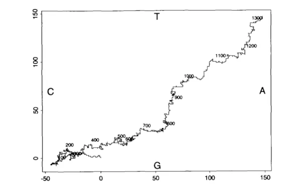
Fig. 1. A random walk representation of a DNA sequence. A move to the right corresponds to an A, a move to the left is a C, an upward move is a T and

a downward move is a G. The corresponding position within the sequence is shown with the help of labels and by changing colors along the curve. This plot, as well as all the other graphical output Included in this paper, has been produced with the statistical package Splus (Becker, Chambers and Wilks, 1988).

distribution of the different nucleotides in a DNA molecule. A cleavage plot shows the cumulative excess of GC's over AT's as one moves along the sequence and thus traces a curve. The choice of these particular pairings is justified because GC and AT are complementary bases. The curve shows the GC-richness within the sequence. In the same figure, a second curve is included, namely the cumulative excess of CT's over GA's. Since C and T are pyrimidines whereas G and A are purines, this curve exhibits the distribution of purines and pyrimidines. A quick scan of this type of plot permits us to determine if any of the nucleotides are over or under represented in various regions of the sequence. In a compressed form, this figure contains the complete information about the base composition of the underlying sequence. In fact, plotting only two curves is sufficient as long as they can move in both directions, thus creating four possible behaviours. A particular base pair can then be inferred from the joint behaviour of the curves. If both curves of a cleavage plot increase, the base must be a C, etc.

The random walk plot is another display based on counting excesses of one type of base over another type. It shows the trajectory of a particle starting at zero that moves either left/right or up/down depending on the type of base. The occurrence of an A moves the curve to the right, a C to the left, a G down and a T up. For each position along the sequence, this plot shows with its horizontal coordinate the excess of A's over C's and with its vertical coordinate the excess of T's over G's. In this

chart, information is lost, because periodic subsequences can lead to a random walk that moves several times over the same ground. For example, a stretch of alternating AC's or TG's would not be identified. The indices of the bases, their positions, are not part of this plot, which is the reason for the information loss. On the other hand, we gain in compactness because a single curve represents the whole sequence and because the scales of the axes are such that details remain visible even for very long sequences. Partial positional information can be incorporated by coloring or labelling. Gates (1985) presents the same idea with a different mapping of base pairs to planar moves.

Figure 1 shows an example using the human HPRT mRNA sequence as discussed in Jolly et al. (1983). This sequence contains the coding part of the gene (657 bases from position 86 through position 742) together with flanking regions (of 674 nucleotides). In the example shown in Figure 1, one notices first a flat part of the curve moving to the left and thus indicating C-richness. On the whole, the curve seems to move along the diagonal from south-west to north-east. This corresponds to a steady increase in the excess of AT's over GC's. Shortly after the end of the coding part of the sequence, one notices a region of more than 100 bases enriched in T's.

Gap plots

A question of interest is to determine whether the positions of bases or of certain base combinations are

Random walk and gap plots of DNA sequences A: 197 times T: 190 times 42

Witt

Fig. 2. These bar charts show the number of times that the lags 1 through

50 occur for the four types of bases in the coding subsequence of the HPRT mRNA. To make the plot more readable, the average number of the lag counts was subtracted before constructing the plot. These means were 56.3, 54.3, 37.1, and 16.9 for the letters A, T, G and C, respectively. If all lags were equally likely between occurrences of A, one would roughly have a mean count of nA(nA—l)/(n—1) for each lag, where nA is

the number of A's and n is the length of the sequence. The observed averages are quite close to these theoretical means. A rough measure of statistical significance could be based on twice the root of the mean number, which supposes an approximate Poissonian behaviour of these counts. Large deviations from the average can be observed for quite big lags. Lag 44, for example, is often seen in the letters A, G, and C, whereas lag 42 sticks out for T. For the letter T, lags that are multiples of three occur more often than average, leading to a striking pattern. Even more pronounced is the period of length 9.

periodic or, more generally, show patterns. A traditional exploratory tool designed for this purpose is the dot matrix plot. Another simple graphical tool to check for patterns is a plot of the lags between occurrences of a letter.

Plotting a single sequence

The sequence AATCATGCAC, for example, has four A's with lags 1, 4, 8, between the first A and the three others; lags 3, 7, between the second and the rest; and lag 4 between the last two A's. Combined, the sequence of A's has once lag 1, once lag 3, twice lag 4, once lag 7, and once lag 8. The gap plot consists in drawing a histogram of these lag counts. If every fifth letter of a sequence were an A, then the most frequently occurring lag between A's would be lag 4, followed by lag 8, by lag 12, etc. This shows how lag counts can exhibit periodic behaviour through peaks and troughs in the lag counts. It is easy to show that these gaps represent the traditional autocovariances of the base sequences consisting of O's and l's obtained from the DNA sequence. The sequence AATCATGCAC, for example, corresponds to the A-sequence 1100100010, to the T-sequence 0010010000, etc. Let x,, x2, ..., xn be the

A-sequence. The autocovariance at lag k is denned as E x, x, + k/n, which is equal to the gap count at lag k divided by n. This connection between gap counts and autocovariances shows that it is very easy to compute the gap counts rapidly and efficiently via the fast Fourier transform. Figure 2 shows the gap plot of the four bases for the coding part of the mRNA sequence that we already used in Figure 1.

Another possible lag statistic could be based on the lags between successive occurrences of a particular base. The maximal and minimal lags give indications of clustering and sparseness and are useful in the analysis of DNA sequences and amino acid sequences (Karlin and Brendel,

1992).

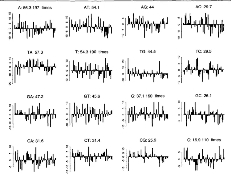
The gap plot can be generalized to lagged cross-covariances between two letters. A DNA sequence corresponds after all to four base sequences and studying the cross-covariances between pairs is the next logical step after exploring the autocovariances. We can ask, what gaps occur between the letters A and T, for example. In the simplistic example of the sequence AATCATGCAC, there are gaps of 2, 5 to subsequent T's, from the second A; gaps of 1 and 4, from the third A; and finally, a gap of 1. Similarly, one can count gaps from T to A, or for any other pair of letters. Figure 3 shows the corresponding gap plot for the coding sequence of the human HPRT mRNA. In Figure 3 we can potentially see many possible patterns and peculiarities. Such patterns may, however, be strengthened in grouping the letters.

Plotting two sequences

It is also quite natural to generalise this type of plot to the case of two sequences. To illustrate, the following simple example suffices. Let the two sequences be AATCGCA and TATAGC. If we are interested in the lag patterns for the A's, we convert them to 1100001 and 010100. We define lag 0 to mean that the sequences are aligned at their left end points. Negative lags are shifts to the right of the second sequence, whereas positive lags are left shifts of the second sequence. Whenever two ones are aligned for a given lag, this indicates the presence of that particular lag. Using our simple example, we note that at lag 0, there is one alignment, namely the A's (or l's) in the second position. At lags - 1 , - 2 and - 4 there are none. At lags - 3 and - 5 there is one. This is the same as saying that from the first and second A in the second sequence, we shift to the right five or three times to get to an A in the first sequence. Among the positive lags a count of one occurs for lags 1, 2 and 3. This follows because the first A in the first sequence must be shifted right once or three time to get to an A in the second sequence, whereas for the second A a shift of two is necessary.

A: 56.3 197 times

r

AT: 54.1 AG:44 AC: 29.7

LJIJIIJII,.

If

TA: 57.3 T: 54.3 190 times TG: 44.5 TC: 29.5

GA: 47.2 GT: 45.6 G: 37.1 160 times GC: 26.1

CA: 31.6 CG: 25.9 C: 16.9 110 times

Fig. 3. These bar charts show the number of times that the lags 1 through 50 occur for all two letter combinations within the coding sequence of the

HPRT mRNA sequence. The height of the bars represent the gap counts minus the average gap count up to lag 50. The averages are indicated in the title of each plot.

Discussion

We have discussed two new plots of DNA sequences. The random walk plot visualises the base composition of a given sequence by plotting it in the form of a random walk. This particular graph exhibits local behaviour along short segments, but is in particular designed to show the global structure of long sequences. The second type of plot is based on counting gaps between the occurrence of bases and exhibits either the lagged correlations within one sequence or between two sequences. This technique is based on the idea of correlations and thus is related to the dot matrix analysis. A dot matrix—in its simplest form— shows a maximum of detail, namely all matches of all pieces of a sequence with all pieces of the other (or the same) sequence. The gap plots included in this paper are a more focused, alternative, way of visualising various patterns in DNA sequences. By applying the techniques of this paper to windowed sequences, the more general

methods obtained will gain in their power to show details, affecting relatively short parts of one or two sequences. References

Barry,D and Hartigan,J.A (1987) Statistical Analysis of Evolution

Statistical Science, 2, 191-207.

Becker.R.A, ChambersJ.M and Wilks.A.R. (1988) The new S

Language. Wadsworth & Brooks/Cole, Pacific Grove, CA.

Doolittle.R.F. (ed.) (1990) Molecular Evolution: Computer Analysis of

Protein and Nucleic Acid Sequences, Vol. 183 (Methods in

Enzymol-ogy). Academic Press, New York

Gates.M.A. (1985) Simpler DNA Sequence Representations. Nature,

316,219.

Gribskov,M. and Devereux,J. (1991): Sequence Analysis Primer. W.H.Freeman, New York.

Jolly.DJ., Okayama.H., Berg.P., Esty,A.C., Filpula,D., Boehlen.P., Johnson.G.G., ShivelyJ.E., Hunkapillar.T. and Friedman.T.B. (1983) Isolation and characterization of a full-length expressible cDNA for human hypoxanthine phosphoribosyl transferase. Proc.

Nail Acad. Sci. USA, 80, 477-481.

Karlin.S. and Brendel,V. (1992) Chance and statistical significance in protein and DNA sequence analysis. Science, 257, 39-49.

Random walk and gap plots of DNA sequences

Sankoff.D. and KruskaU.B. (1983) Time Warps, String Edits, and

Macromolecules- The Theory and Practice of Sequence Comparison.

Addison-Wesley, Reading, MA.

ShepherdJ.C.W. (1981): Method to determine the reading frame of a protein from the purine/pyrimidine genome sequence and its possible evolutionary justification. Proc. Natl Acad. Sci. USA, 78, 1596-1600. Tukey,J.W. (1986) Volume V of the Collected WorksofJohn W.Tukey. In.

Cleveland.W.S (ed.), Wadsworth & Brooks/Cole, Monterey, CA.

Received on December 17, 1994, revised on July 19, 1995, accepted on August 11, 1995