HAL Id: hal-02163492
https://hal.archives-ouvertes.fr/hal-02163492
Preprint submitted on 24 Jun 2019HAL is a multi-disciplinary open access
archive for the deposit and dissemination of sci-entific research documents, whether they are pub-lished or not. The documents may come from teaching and research institutions in France or abroad, or from public or private research centers.
L’archive ouverte pluridisciplinaire HAL, est destinée au dépôt et à la diffusion de documents scientifiques de niveau recherche, publiés ou non, émanant des établissements d’enseignement et de recherche français ou étrangers, des laboratoires publics ou privés.
Lempel-Ziv complexity of the pNNx statistics -an
application to neonatal stress
Matej Šapina, Chandan Karmakar, Karolina Kramarić, Marcin Kośmider,
Matthieu Garcin, Dario Brdarić, Krešimir Milas, John Yearwood
To cite this version:
Matej Šapina, Chandan Karmakar, Karolina Kramarić, Marcin Kośmider, Matthieu Garcin, et al.. Lempel-Ziv complexity of the pNNx statistics -an application to neonatal stress. 2019. �hal-02163492�
Lempel-Ziv complexity of the pNNx statistics – an application to neonatal stress
Matej Šapina1,2,3, Chandan Karmakar4, Karolina Kramarić1,2,3, Marcin Kośmider5, Matthieu
Garcin6, Dario Brdarić3,7, Krešimir Milas1,2, John Yearwood4
1University hospital Osijek, Pediatric Clinic, J. Huttlera 4, 31000 Osijek, Croatia, 2Medical
faculty Osijek, Osijek, J. Huttlera 4, 31000 Osijek, Croatia, 3Faculty of Dental medicine and
Health, Crkvena 21, 31000 Osijek, Croatia, 4School of Information Technology, Deakin
University, Geelong, Australia, 5Institute of Physics, University of Zielona Gora, Prof. Szafrana
4a, 65-516 Zielona Gora, Poland, 6Léonard de Vinci Pôle Universitaire, Research center, 92916
Paris La Défense, France, 7Institute of Public Health for the Osijek Baranya County, Drinska 8,
31000 Osijek, Croatia
Corresponding author:
Matej Šapina, MD
J. Huttlera 4, 31000 Osijek, Croatia
Phone: 00 385 95 556 78 76
ABSTRACT
Among the existing measures of heart rate variability (HRV), the pNN50 statistics is one
of the most commonly reported. However, it is only a single member of a much larger family
of HRV measures - the pNNx statistics. In this research pNNx was further extended, combining
it with the Lempel-Ziv complexity (LZ76) in a controlled neonatal stress framework. Forty
healthy newborns were recorded undergoing two different types of stress stimuli – a routine
heel stick blood sampling, and a dull heel pressure stimulation. Instead of relying on a single
value, the entire spectrum from pNN1 to pNN100 was calculated, along with LZ76 derived
from binarized sequences for each NN. The results of this study show a downward shift of the
pNNx curves when newborns are stressed, with reduced LZ76 complexity when stressed.
When ROC curves were utilized for the pNNx statistics and LZ76, however, the highest AUC
values were observed when both measures were combined, with the highest AUC values of
0.88 (0.80-0.94) and 0.85 (0.74-0.91) for discriminating resting states from stress phases.
Combining the widely used pNNx statistics with LZ76 extends the existing HRV toolbox, and
shows a promising application in recognizing acute neonatal stress.
Keywords: Heart rate variability, Lempel-Ziv Complexity, Newborns, Stress, Cardiac inter-beat
INTRODUCTION
Children differ from adults in various ways. Due to their dynamic developmental
changes, the pediatric population is subjected to higher environmental polutants. The lower
the newborn’s gestational age, the less is their adaptive tolerance, leading to stress
responses, which would not occur in the mature human 1,2.
For a long period, a paradigm existed regarding the lack of capabilities of newborns for
feeling pain. But when, in the late 1980s, Anand and Hickey published their seminal work on
neonatal pain, the traditional views started to change 3. However, newborn pain still remains
undertreated 4 . Pain induces a stress response, which changes the bodies' homeostasis, and
can have both a short- and long-term effect on the developing body 5,6. When being stressed,
a hormonal response is generated, leading to an increase of heart and respiratory rate, blood
pressure fluctuations, changing the cerebral blood flow, and in the long run, even epigenetic
changes might occur 6-8.
Acute stress and newborn pain is commonly assesed using pain scales 9. Unfortunately,
relying only on pain scales might suffer from lack of objectivity, due to the subjective or
incosistent pain assesment, and further due to the limited knowledge of the nature how
neonates response to pain 10. Both term and preterm newborns in the intensive care unit
(NICU) are continuously being monitored using different devices, which can be used as an aid
for a more objective stress and pain assessment 11,12.
Heart rate variability (HRV) is the variability of duration of consecutive cardiac cycles
originating from the sinus node. In the last decades, HRV showed itself useful as both a basic
science reasearch tool for the assessment of the autonomic nervous system (ANS), as well as
statistical methods, which can be roughly divided into: time domain, frequency domain, and
nonlinear methods 14.
The time domain analysis can be further divided as measures directly and indirectly
derived from the RR interval recording. Among the latter, probably the simplest to be
calculated is the widely, and nowadays standardly used measure – the pNN50 statistic. The
pNN50 statistics was initially developed by Ewing in 1984. It is defined as the proportion
consecutive normal sinus (NN) intervals whose differences exceed 50 ms. As such it was
proposed to be a measure of parasympathetic activity 15. Since then, the pNN50 proved itself
to be a useful measure of HRV in various basic and clinical research. However, the fixed
threshold of 50 ms, was only arbitrarily recommended due to the easiness of calculation 16.
Therefore, the pNN50 statistic is only a single member of a much larger family of HRV
measures – the pNNx family. Mietus et al. first investigated the relationship of other
thresholds compared to the standard pNN50, trying to find a more robust discrimination
between healthy and diseased groups of patients 16. As more evidence was gathered, lower
NNx values are being more frequently reported along with pNN50.
Time and frequency domain are often not sufficient to describe the complex heart rate
variability dynamics, due to the complex interactions of mechanisms involved in
cardiovascular regulations 17. Various nonlinear methods have been proposed in the analysis
of HRV, among which complexity measures play a particular role 18. The Lempel Ziv (LZ)
complexity is a measure to assess the algorithmic complexity, defined according to the
Information Theory as the least amount of information to describe a binary string 19. With the
time evolution of the extending string, the LZ complexity quantifies the rate of new patterns
This research is based on the notion that even simple statistics such as the pNNx
statistics can exhibit complex structures of the heart rate variability. We are particularly
interested in applying the LZ complexity to a coarse-grained time series from the binarized
pNNx statistics spectrum. Thus, we hypothesize the simultaneous application of pNNx and LZ
will provide more useful discriminating properties than each statistic alone.
SUBJECTS AND METHODS
Ethical statement
The research was accepted by the University hospital Clinic Osijek ethical committee,
and informed consents were obtained from all research participant’s parents or guardians.
The study protocol
The patient’s demographics and study protocol have been reported previously 22-25.
Shortly, forty healthy term neonates, born through vaginal delivery, with an APGAR score >9/9
were included in the study. The study sample consisted of 21 females and 19 males with birth
weight 3542.05 ± 339.09 g, and were randomly chosen over a three months period from the
Osijek University Clinic pediatrics clinic's maternity ward. Except two female twins, the rest of
the participants were singletons. The study was performed when the newborns reached 72
hours postnatal age, just prior discharge, which is the recommended chronological age for
routine phenylketonuria and congenital hypothesis screening. Besides the routine screening
heel stick blood draw, none of the newborns underwent any other procedural pain.
The experimental protocol is divided into three parts: a) dummy stimulation, b) the
sharp pain - heel stick, c) the treatment; however, the treatment part was not included in the
and an interventional phase (Phases 2 and 4). The protocol was carried out in a serialized
manner: Phase 1) - 10 minutes of resting, followed by Phase 2) the dummy stimulation phase,
where intermittent pressure onto the newborn's heel was applied, mimicking a heel stick
blood drawing without blood sampling. The duration of Phase 2 was fixed at 90 seconds, which
was the average time for the nurse to perform the blood drawing. At the end of Phase 2, Part
b) of the experiment began. Phase 3 was the second resting phase, lasting 10 minutes,
followed by the heel stick blood drawing procedure (Phase 4). Phase 4 differed in duration,
because of the variability of time needed to collect the least amount of blood for the metabolic
screening.
During the entire procedure, the RR intervals were collected with a light weight
high-resolution sampling device (Firstbeat Bodyguard 2, Firstbeat TechnologiesLtd, Jyvaskyla,
Finland, sampling frequency 1024 Hz). The recordings were further visually inspected, and
after artifact removal, the data was ready for analysis. Each infant was fed with breast milk or
formula, and positioned in supine position in a quiet room to minimize the external artefacts.
The pNNx statistics and the Lempel-Ziv complexity
We simply calculated the pNNx statistics as the number of consecutive RR (NN)
intervals differing by more than x ms in the entire recording divided by the total number of all
RR intervals (nNN):
𝑝𝑁𝑁𝑥 =Card(i ≤ 𝑛𝑁𝑁, |RR𝑖+1 − RR𝑖| > x )
Binarization
A binarized sequence is the starting point to obtain both the pNNx statistics and LZ
complexity. From the original RR interval time series, differences between two successive RR
intervals greater than a threshold value x are replaced with 1, and values lesser or equal to x,
with 0. Therefore, for each threshold x, both the pNNx and LZ complexity can be calculated:
1. The preprocessing step consists in calculating the first absolute differences between
successive RR intervals. For example, the first absolute differences of the time series
RR ≡ (343, 350, 349, 400, 551) equal ΔRR ≡ (7, 1, 51, 151).
To find the pNN50, the number of elements greater than 50 is divided by the total
number of elements, which in this example is pNN50 = 0.5. Additionally, to calculate
the pNN2, the numbers of elements greater than 2 is divided by the total numbers of
elements in the time series, which is here pNN2 = 0.75.
2. After defining the threshold number x, a sequence can be binarized by replacing the
elements greater than x in the ΔRR time series with 1, and the others with 0.
If x = 50, the first absolute differences time series, ΔRR ≡ (7, 1, 51, 151), is converted
into:
ΔRR01(50) ≡ (0, 0, 1, 1).
Additionally, if x = 2, the time series becomes:
ΔRR01(2) ≡ (1, 0, 1, 1).
3. After obtaining the binary sequence, the standard and normalized LZ76 can be
LZ76
The LZ is often used as a parameter to estimate the complexity of discrete time series
26. The general idea behind it is quite natural: time series consist of repeated basis patterns of
various sizes so the series can be decomposed on these patterns. Therefore, LZ is the number
of basis patterns. In this work, the original LZ76 was chosen for estimating the complexity. We
further describe, in an easy way, how LZ76 algorithm works and how complexity can be
calculated.
1. The original sequence S = a1 a2 a3 … an, where ai is a number 0 or 1, and n is the
number of elements in the time series, can be divided into subsequences:
s(i,j) = ai ai+1 ... aj, where 𝑖 ≤ 𝑗. The sequence S can then be written as the sum of
subsequences: S = s(1,i) s(i+1, j) ... s(k+1, n).
2. There are a lot of possibilities to divide the original time sequence S in subsequences
s. In LZ76 algorithm S is divided into subsequences that fulfill the relation: s(i,j) is not a
subsequence of s(1, j-1). Only the last subsequence can be observed previously if there
are not enough data.
3. The number of unique subsequences is defined as LZ complexity. For example, a
binary sequence S = 1001111011000010 can be rewritten as:
1|0|01|1110|1100|0010 which results in a complexity of S equal to 6. The binary
sequence S=111111 has complexity 2 because, according to the second step in the
The complexity depends on the time series length. To compare time series differing in
length, it is necessary to define normalized complexity 27,28. It has been shown that the upper
bound of complexity c(N) is defined by:
𝑐(𝑆) < 𝑁
(1 − εN)𝑙𝑜𝑔𝜎(𝑁)
where N is the length of sequence and σ is the number of different symbols in sequence 19.
For a binary sequence σ = 2 (0 and 1), εN is a slowly decaying function of N, and for 𝑁 → ∞, ε𝑁
→ 0, therefore the normalized LZ76 complexity, C(S), can be calculated as 19.
𝐶(𝑆) =𝑐(𝑆)𝑙𝑜𝑔𝜎(𝑁) 𝑁 .
The impact of different lengths
It should be noted that the LZ76 complexity highly depends on the length of the strings.
Although the first three phases of our experiment could be controlled in terms of length of
time, due to the variability of the RR intervals lengths, two patients with the same length of
the recordings did not have the same numbers of RR intervals. Therefore, the average (±SD)
number of RR intervals in our dataset was as follows: Phase 1 was 1284.13±149.23, Phase 2
229.93±43.03, Phase 3 1323.6±193.2, and Phase 4 411.63±193.31. This discrepancy of lengths
might be a major drawback for the results, prone to biased conclusions, but could be
minimized with normalization of LZ76 complexity.
To overcome the potential bias that results from the different lengths of the
recordings, and not to discard any data, besides normalizing the LZ76 complexity, the shortest
recording (94 RR intervals in one patient of Phase 4) was used as a reference length.
Specifically, the shortest length was rounded to 90 datapoints. Instead of randomly selecting
was calculated in each recording using a box of length of 90 datapoints with 89 datapoints
overlapping. Finally, after calculating the last box in a particular recording, the average of the
obtained normalized LZ76 complexities were used as a measure of complexity for the
recording.
Statistical analysis
The data were analyzed with Python 3 and the Matlab R2007a softwares. The
normality of the distributions was assessed using the Kolmogorov-Smirnov test. The data are
descriptively presented with means and standard deviations. Repeated measures ANOVA, was
applied to assess the mean differences of the pNNx statistics and LZ76 complexity between
phases. A ROC curve analysis was performed to test the model's diagnostic properties of pNNx
and LZ76 as well as their combination, to differentiate stress phases (Phase 2 and 4) from the
first baseline phase (Phase 1). P values less than 0.05 were considered statistically significant.
Since 𝑝𝑁𝑁𝑥 and 𝐿𝑍76 were calculated for 𝑥 = 1. . .100, the ROC calculation resulted
in a series of 100 elements. Based on this ROC series 𝑅𝑂𝐶𝐴𝑟𝑒𝑎, we derived new features from
pNNx and LZ76 values as follows:
𝑝𝑁𝑁𝑥𝑎−𝑏 ̅̅̅̅̅̅̅̅̅̅̅̅ = 1 𝑏 − 𝑎 + 1∑ 𝑝𝑁𝑁𝑥𝑖 𝑏 𝑖=𝑎 𝐿𝑍76𝑎−𝑏 ̅̅̅̅̅̅̅̅̅̅̅ = 1 𝑏 − 𝑎 + 1∑ 𝐿𝑍76𝑖 𝑏 𝑖=𝑎
where, 𝑎 and 𝑏 are the starting and ending index of a sequence that meets the criteria
∀𝑖: 𝑅𝑂𝐶𝐴𝑟𝑒𝑎𝑖 ≥ 0.7 | 𝑎 ≤ 𝑖 ≤ 𝑏 and 𝑏 − 𝑎 + 1 ≥ 5. The descriptive statistics (mean and
standard deviations), 𝑝 value and ROC area of these features were then calculated in the same
combinations of these features namely, I) all pNNx derived features; II) all LZ76 derived
features; and III) both pNNx and LZ76 band features, were then computed using linear
RESULTS
The results of the pNNx and LZ76 analysis are presented in the tables and further
reported in figures. Due to the wide range, the results for the first ten NNx values are reported,
while the following NNx values are reported rounded to the nearest tenth, i.e. 20, 30, 40 etc.
Table 1. contains mean values and standard deviation of the varying pNNx results across the
different phases of the experiment. A common feature of all phases is the high percentage of
pNNx values at lower NNx values, which strongly decreases when increasing the NNx values
(Figure 1).
However, the stress phases can be visually differentiated from resting phases. An
overlap between the resting phases, and both stress phases is observed. The difference of the
curves is the lowest at the beginning and at the end of the NNx spectrum, and the widest at
levels between NN10 and NN20.
The highest pNNx values are trivially observed for each phase at NN1. pNN1 values for
the resting phases (phase 1 - 84.15±10.02, phase 3 - 81.73±12.48) were significantly higher
than at the resting phases (phase 2 - 73.63±12.53, phase 4 - 69.13±15.51), p<0.001.
The value of the standard pNN50 at phase 1 and phase 3 were close to each other
(4.53±6.46, and 4.93±8.8, respectively), similar to the values of pNN50 of phase 1 and phase
3 (2.18±5.09 2.38±4.23, respectively), p=0.021.
Considering statistical significance, a slow increase of p-values is observed with
increasing NNx levels. The lowest p-values are seen at the first twenty NNx levels, while a
cut-off is observed around NN70 (0.048), showing no statistically significant differences of pNNx
The shape of the normalized LZ76 values for different pNNx values represents a right
tailed function, with the peak values at lower pNNx values, and lags between phases (Figure
2). The highest LZ76 values for the resting phases are observed at NN5 and NN6 (phase 1: NN5
- 0.98±0.16, NN6 - 0.98±0.17, phase 3: NN5 - 0.93±0.19, NN6 - 0.93±0.21), and for the stress
phases at NN3 (phase 2 - 0.96±0.17, phase 4 - 0.93±0.18). At NN50 LZ76 were significantly
lower (phase 1 - 0.32±0.2, phase 3 - 0.31±0.24), with both resting phases having similar value,
as well as the stress phases (phase 2 - 0.24±0.18, phase 4 - 0.23±0.14). Nonsignificant p-values
were observed at NN3, NN4, and at NN leves greater than 80 (Table 2.).
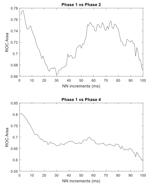
The results of the ROC analysis are presented in Figures 3 and 4. A bimodal distribution
is observed in the value of AUC levels with varying NN increments for the pNNx statistics.
Regarding the properties differenciating Phase 1 from Phase 2, the highest AUC were observed
at lower NN increments, followed by a fall with AUC levels bellow 0.68, NN30 having the
smallest AUC value. An upward trend is further observed, with AUC levels plateauing between
NN50 and NN75, followed again by a decrease in AUC levels.
A similar pattern is observed differenciating Phase 1 and Phase 4, however, the
bimodal distribution flattened. The highest AUC values were observed at the smallest NN
increments, followed by a slight decrease and then by an upward trend between NN 40 and
60. In general, except for the lowest NN increment, the AUC values were lower when
discriminating Phase 1 from Phase 4, than Phase 1 from Phase 2.
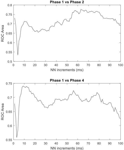
The AUC values of the LZ76 complexity are presented in Figure 4. A similar pattern of
the AUC values is observed when discriminating Phase 1 from Phase 2, and Phase 1 from Phase
4. A sudden decrease of AUC values is observed in both cases at lower NN increments. The
while the highest values differentiating Phase 1 from Phase 4 are observed with NN
increments between 10 and 20.
Performances of derived features and their different combinations are presented in
Table 3 and 4. Mean value of individual feature is higher in baseline phase (Phase 1) than
stressed phase (Phase 2 and 4). The 𝑝 value clearly indicates that values of all features are
statistical significantly different (𝑝 < 0.05) between baseline and stressed phases. The ROC
area (≥ 0.71) also supports the findings. Table 4 shows the performance of different
combinations of derived features. It is obvious that combining features together improves the
differentiation capacity of derived features. The maximum ROC area between Phase 1 and 2
is 0.88 (C.I.: 0.80-0.94) using all four derived features compared to 0.75 for the single best
feature (𝑝𝑁𝑁𝑥̅̅̅̅̅̅̅̅̅̅̅̅̅). Similarly, combinations of all derived features shows higher ROC area 1−16 0.85 (C.I.: 0.75-0.91) than 0.76 obtained using the best single feature (𝑝𝑁𝑁𝑥̅̅̅̅̅̅̅̅̅̅̅̅̅) to 1−15 differentiate Phase 1 and 4.
DISCUSSION
The first study stating the limitations of a single threshold value of 50 ms was
conducted by Mietus et al 16. Their findings showed that the selection of a wide range of
thresholds would be more beneficial instead on relying on a single member of the pNNx
family.
When comparing the graphical presentations of the pNNx values between healthy
subjects and those suffering from congestive heart failure (CHF), a downward shift of the
curves of CHF patients was observed 16. This finding can be related to the results obtained in
our study (Figure 1). The slope of the mean pNNx curves varies, with the stress phases
decreasing pNNx much faster than resting phases, resulting in a downward shift of the stress
phases curves.
Mietus et al. also stated that NNx<8 might be likely of limited reliability in ECG data
obtained with lower sampling rates, and potentially useful at higher sampling rates 16. The
monitor used in this study had a sampling rate of 1024 Hz, and the obtained results show that
very low thresholds can be applied using a high-resolution monitor, finding subtle variations
in the heart rate
Generalizing the pNNx family opens further possibilities of more complex analysis. Yi
et al. used a symbolic dynamics approach to the analysis of the pNNx statistics comparing
healthy subjects, with patients suffering from atrial fibrillation (AF) and CHF patient group 29.
The mean pNNx curves were similar to the results reported by Mietus et al., while the curve
of patients suffering from atrial fibrillation showed a slow negative downward trend, lacking
that the optimal threshold for distinguishing healthy from sick patients would be between 10
and 25, being far below from 50 ms 29.
In our study, we considered the application of LZ complexity analysis as an alternative
approach to the symbolic dynamics of a coarse-grained time series based on the binarized
pNNx sequence.
The conventional 50 ms threshold showed statistically significant differences between
resting and stressed newborns. For every threshold level, the complexity was greater in the
resting phases, except for NN>1 to NN>4. However, no statistical significance differences were
observed for NN3 and NN4.
The interpretation of the LZ complexity results can be explained in terms of a random
sequence or the quantity of frequency components. The complexity of a completely random
sequence tends to be 1, while a periodic sequence has a complexity 0. The greater the
complexity of a sequence is, the more irregular and random the sequence is, and in contrary,
the more periodic or the less regular the sequence is, the lesser is its complexity30. The results
of the LZ76 complexity can be related to the pNNx statistics. A high threshold contains only a
small fraction of the beats greater than the defined threshold itself, while a low threshold
contains a majority of the values. For example, the probability of NN>1 in phase 1 is 84.15%,
while the probability of NN>100 is only 0.64%. That means, there is a higher probability to
obtain a uniform binarized sequence with pNN100, than pNN1. Those low frequency
components result in a very low complexity of the higher threshold series.
The physiological interpretation of this behavior is not completely understood, and can
currently only be speculated. HRV analysis has been already applied in the neonatal
framework, using a multi-lag tone entropy, asymmetric detrended fluctuation, asymmetric
approach22-25. The increase of the negative scaling exponent, depicting higher autocorrelation,
and the Poincaré plot asymmetry showed a higher contribution of accelerations within the RR
interval time series, while the multi-lag tone-entropy showed a decrease of the
parasympathetic, and an increase of the sympathetic branch of the autonomic nervous system
22-24. The reduction of pNNx values, and a consequential downward shift of the curve probably
resulted as a modulation of the autonomic nervous system in stressed newborns, due to the
reduction of the tone of the parasympathetic and increase of the sympathetic tone. The
different complexities within resting and stressed newborns are a result of both a modulation
of the autonomic nervous system and coarse-grained pNNx time series. Unfortunately,
although the differences in the complexities were found between resting and stressed
newborns, an explicit physiological interpretation cannot be stated yet. The reason for this is
the wide range of NN thresholds, but in general, for threshold levels higher than 4 ms, stress
results in a decreased complexity. This finding is consistent with the reduction of entropy,
reflecting the reduction of the parasympathetic and increasing the sympathetic activity 23.
Another aim of this study is to utilize the newly observed feature extraction as a
diagnostic tool, differentiating stressed from resting newborns. Questions may arise: how
would it be beneficial using a complex method such as the LZ76 complexity, instead of an
easy-to-calculate, proven method like pNNx? The results of the ROC analysis show that the highest
pNNx value for discriminating stressed from resting infants are at lower threshold levels. The
AUC levels for LZ76 were even lower. However, when combined, different features from the
pNNx family and LZ76 complexity resulted in an AUC of 0.88 with an upper bound of the
confidence interval up to 0.94 for discriminating phase 2 from phase 1, and AUC of 0.85 with
a confidence interval up to 0.91, for discriminating phase 4 from phase 1. Although the
different stress phases, it should be noted that different features were extracted to obtain a
useful model. The reason for that difference is the duration and type of the applied stress. In
phase 2, the heel was bluntly stimulated, while in phase 4, a sharp heel lance was applied,
followed with intermittent heel pressing, to obtain the lowest amount of blood sufficient for
metabolic screening. Nevertheless, the findings suggest that a combination of pNNx and LZ76
provides better results in discriminating stressed from resting newborns than each statistic
alone.
Although this study is a result of a controlled acute stress, the findings show a
promising application in real life. If a newborn is suspected to have a pathological condition,
it will definitely experience procedural pain, and with a worsening condition, the newborn will
be monitored in intensive care units using a heart rate monitor. One of the most illustrative
examples using pNNx and LZ76, along with other HRV features would be analgesia and
sedation titration. Both have various side effects which require caution when being applied,
therefore it is crucial to have the child monitored, without unwanted exaggeration. Besides
having a potential application in the pediatric field, the binarization of the pNNx time series
opens possibilities for applying different nonlinear and complexity measures, i.e. LZ78,
symbolic dynamics, entropy measures etc.
In conclusion, a novel HRV model was applied on neonates undergoing acute stress.
This study stresses the importance of not solely relying on a single fixed threshold, but on a
wide range of numbers. The traditional pNNx statistics can be further extended applying LZ76
complexity, which when combined makes it useful as an extension of the traditional methods
Acknowledgements
We thank dr. Marko Pirić, for their help in conducting the research.
Conflict of interest
REFERENCES
1. Gunnar MR, Hertsgaard L, Larson M, Rigatuso J. Cortisol and behavioral responses to
repeated stressors in the human newborn. Dev. Psychobiol. 24:487-505, 1991.
2. Kramarić K, Šapina M, Milas V, et al. The effect of ambient noise in the NICU on cerebral
oxygenation in preterm neonates on high flow oxygen therapy. Signa Vitae. 13:52-56, 2017.
3. Anand KJ, Hickey PR. Pain and its effects in the human neonate and fetus. N. Engl. J.
Med. 317:1321-1329, 1987.
4. Bauchner H, May A, Coates E. Use of analgesic agents for invasive medical procedures
in pediatric and neonatal intensive care units. J. Pediatr. 121:647-649, 1992.
5. Grunau RE, Holsti L, Haley DW, et al. Neonatal procedural pain exposure predicts lower
cortisol and behavioral reactivity in preterm infants in the NICU. Pain. 113:293-300, 2005.
6. Hatfield LA. Neonatal pain: What's age got to do with it? Surg. Neurol. Int. 5:S479,
2014.
7. Vesoulis ZA, Mathur AM. Cerebral autoregulation, brain injury, and the transitioning
premature infant. Front. Pediatr. 5:64, 2017.
8. Stone LS, Szyf M. The emerging field of pain epigenetics. Pain. 154:1-2, 2013.
9. Blauer T, Gerstmann D. A simultaneous comparison of three neonatal pain scales
during common NICU procedures. Clin. J. Pain. 14:39-47, 1998.
10. Boyle EM, Freer Y, Wong CM, McIntosh N, Anand K. Assessment of persistent pain or
distress and adequacy of analgesia in preterm ventilated infants. Pain. 124:87-91, 2006.
11. Storm H. The capability of skin conductance to monitor pain compared to other
physiological pain assessment tools in children and neonates. Pediatric and Therapeutics.
12. Faye PM, De Jonckheere J, Logier R, et al. Newborn infant pain assessment using heart
rate variability analysis. Clin. J. Pain. 26:777-782, 2010.
13. Pongiglione G, Fish FA, Strasburger JF, Benson DW. Heart rate and blood pressure
response to upright tilt in young patients with unexplained syncope. J. Am. Coll. Cardiol.
16:165-170, 1990.
14. Cardiology TFotESo. Heart rate variability, standards of measurement, physiological
interpretation, and clinical use. Circulation. 93:1043-1065, 1996.
15. Ewing DJ, Neilson J, Travis P. New method for assessing cardiac parasympathetic
activity using 24 hour electrocardiograms. Heart. 52:396-402, 1984.
16. Mietus J, Peng C, Henry I, Goldsmith R, Goldberger A. The pNNx files: re-examining a
widely used heart rate variability measure. Heart. 88:378-380, 2002.
17. Voss A, Schulz S, Schroeder R, Baumert M, Caminal P. Methods derived from nonlinear
dynamics for analysing heart rate variability. Philos. Trans. Royal Soc. A. 367:277-296, 2008.
18. Sassi R, Cerutti S, Lombardi F, et al. Advances in heart rate variability signal analysis:
joint position statement by the e-Cardiology ESC Working Group and the European Heart
Rhythm Association co-endorsed by the Asia Pacific Heart Rhythm Society. Ep Europace.
17:1341-1353, 2015.
19. Lempel A, Ziv J. On the complexity of finite sequences. IEEE Trans. Inf. Theory.
22:75-81, 1976.
20. Ferrario M, Signorini MG, Magenes G. Complexity analysis of the fetal heart rate
variability: early identification of severe intrauterine growth-restricted fetuses. Med. Biol. Eng.
Comput. 47:911-919, 2009.
21. Fernández A, López-Ibor M-I, Turrero A, et al. Lempel–Ziv complexity in schizophrenia:
22. Kramarić K, Šapina M, Garcin M, et al. Heart rate asymmetry as a new marker for
neonatal stress. Biomed. Signal Process Control. 47:219-223, 2019.
23. Šapina M, Karmakar CK, Kramarić K, et al. Multi-lag tone–entropy in neonatal stress. J.
Royal Soc. Interface. 15:20180420, 2018.
24. Šapina M, Kośmider M, Kramarić K, et al. Asymmetric detrended fluctuation analysis in
neonatal stress. Physiol. Meas. 39:085006, 2018.
25. Šapina M, Garcin M, Kramaric K, Milas K, Brdaric D, Piric M. The Hurst exponent of
heart rate variability in neonatal stress, based on a mean-reverting fractional Lévy stable
motion. 2017.
26. Aboy M, Hornero R, Abásolo D, Álvarez D. Interpretation of the Lempel-Ziv complexity
measure in the context of biomedical signal analysis. IEEE Trans. Biomed. Eng. 53:2282-2288,
2006.
27. Ziv J, Lempel A. Compression of individual sequences via variable-rate coding. IEEE
Trans. Inf. Theory. 24:530-536, 1978.
28. Rapp P, Cellucci C, Korslund K, Watanabe T, Jimenez-Montano M. Effective
normalization of complexity measurements for epoch length and sampling frequency. Phys
Rev. E. 64:016209, 2001.
29. Yi S-H, Park K-T, Yoo C-S, Jeon G-R. Implementation of the Real-time Algorithms Based
on the Symbolic Dynamics of a Coarse-grained Heart Rate Variability in Ubiquitous Health Care
Systems. Paper presented at: World Congress on Medical Physics and Biomedical Engineering
20062007.
30. Wang J, Cui L, Wang H, Chen P. Improved complexity based on time-frequency analysis
TABLES
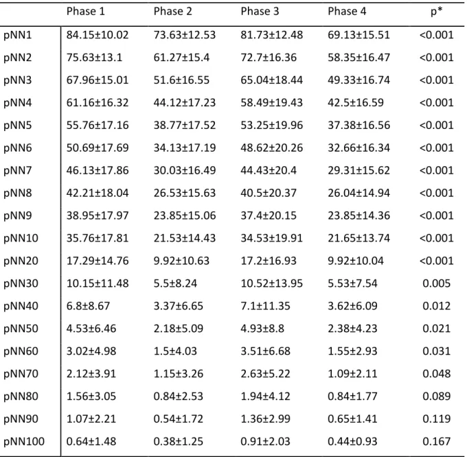
Table 1. Mean ± SD (standard deviation) of pNNx values (in percentage) across the different phases of the protocol with varying pNNx
Phase 1 Phase 2 Phase 3 Phase 4 p* pNN1 84.15±10.02 73.63±12.53 81.73±12.48 69.13±15.51 <0.001 pNN2 75.63±13.1 61.27±15.4 72.7±16.36 58.35±16.47 <0.001 pNN3 67.96±15.01 51.6±16.55 65.04±18.44 49.33±16.74 <0.001 pNN4 61.16±16.32 44.12±17.23 58.49±19.43 42.5±16.59 <0.001 pNN5 55.76±17.16 38.77±17.52 53.25±19.96 37.38±16.56 <0.001 pNN6 50.69±17.69 34.13±17.19 48.62±20.26 32.66±16.34 <0.001 pNN7 46.13±17.86 30.03±16.49 44.43±20.4 29.31±15.62 <0.001 pNN8 42.21±18.04 26.53±15.63 40.5±20.37 26.04±14.94 <0.001 pNN9 38.95±17.97 23.85±15.06 37.4±20.15 23.85±14.36 <0.001 pNN10 35.76±17.81 21.53±14.43 34.53±19.91 21.65±13.74 <0.001 pNN20 17.29±14.76 9.92±10.63 17.2±16.93 9.92±10.04 <0.001 pNN30 10.15±11.48 5.5±8.24 10.52±13.95 5.53±7.54 0.005 pNN40 6.8±8.67 3.37±6.65 7.1±11.35 3.62±6.09 0.012 pNN50 4.53±6.46 2.18±5.09 4.93±8.8 2.38±4.23 0.021 pNN60 3.02±4.98 1.5±4.03 3.51±6.68 1.55±2.93 0.031 pNN70 2.12±3.91 1.15±3.26 2.63±5.22 1.09±2.11 0.048 pNN80 1.56±3.05 0.84±2.53 1.94±4.12 0.84±1.77 0.089 pNN90 1.07±2.21 0.54±1.72 1.36±2.99 0.65±1.41 0.119 pNN100 0.64±1.48 0.38±1.25 0.91±2.03 0.44±0.93 0.167 *Repeated measures ANOVA
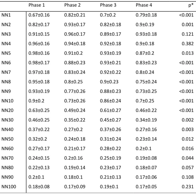
Table 2. Mean ± SD (standard deviation) of LZ76 values across the different phases of the protocol with varying pNNx
Phase 1 Phase 2 Phase 3 Phase 4 p* NN1 0.67±0.16 0.82±0.21 0.7±0.2 0.79±0.18 <0.001 NN2 0.82±0.17 0.93±0.17 0.82±0.18 0.9±0.19 0.001 NN3 0.91±0.15 0.96±0.17 0.89±0.17 0.93±0.18 0.121 NN4 0.96±0.16 0.94±0.18 0.92±0.18 0.9±0.18 0.382 NN5 0.98±0.16 0.91±0.2 0.93±0.19 0.87±0.2 0.013 NN6 0.98±0.17 0.88±0.23 0.93±0.21 0.83±0.23 <0.001 NN7 0.97±0.18 0.83±0.24 0.92±0.22 0.8±0.24 <0.001 NN8 0.95±0.18 0.8±0.25 0.9±0.23 0.75±0.24 <0.001 NN9 0.93±0.19 0.77±0.26 0.88±0.23 0.73±0.25 <0.001 NN10 0.9±0.2 0.73±0.26 0.86±0.24 0.7±0.25 <0.001 NN20 0.63±0.25 0.49±0.24 0.61±0.27 0.46±0.22 <0.001 NN30 0.46±0.25 0.35±0.22 0.45±0.27 0.34±0.19 0.002 NN40 0.37±0.22 0.27±0.2 0.37±0.26 0.27±0.16 0.003 NN50 0.32±0.2 0.24±0.18 0.31±0.24 0.23±0.14 0.012 NN60 0.27±0.17 0.21±0.17 0.28±0.22 0.2±0.1 0.016 NN70 0.24±0.15 0.2±0.16 0.25±0.19 0.19±0.08 0.044 NN80 0.22±0.13 0.19±0.14 0.23±0.17 0.18±0.07 0.057 NN90 0.2±0.1 0.18±0.1 0.21±0.13 0.17±0.06 0.108 NN100 0.18±0.08 0.17±0.09 0.19±0.1 0.17±0.05 0.231 *Repeated measures ANOVA
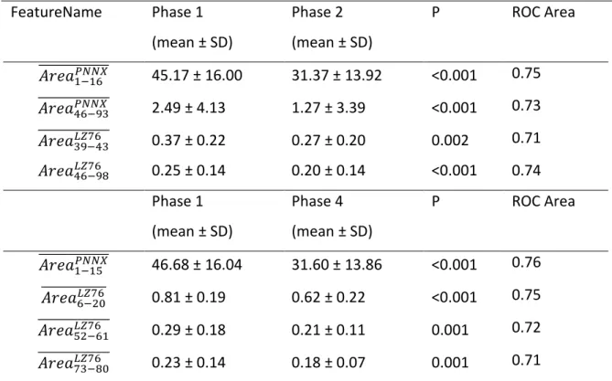
Table 3. Mean ± SD (Standard Deviation) values of band features calculated from pNNx and
LZ16 profiles. P value calculated using non-parametric Mann-Whitney U test. ROC Area shows
the phase differentiating (Phase 1 vs Phase 2 or Phase 1 vs Phase 4) capability of individual
feature. FeatureName Phase 1 (mean ± SD) Phase 2 (mean ± SD) P ROC Area 𝐴𝑟𝑒𝑎1−16𝑃𝑁𝑁𝑋 ̅̅̅̅̅̅̅̅̅̅̅̅̅ 45.17 ± 16.00 31.37 ± 13.92 <0.001 0.75 𝐴𝑟𝑒𝑎46−93𝑃𝑁𝑁𝑋 ̅̅̅̅̅̅̅̅̅̅̅̅̅ 2.49 ± 4.13 1.27 ± 3.39 <0.001 0.73 𝐴𝑟𝑒𝑎39−43𝐿𝑍76 ̅̅̅̅̅̅̅̅̅̅̅̅̅ 0.37 ± 0.22 0.27 ± 0.20 0.002 0.71 𝐴𝑟𝑒𝑎46−98𝐿𝑍76 0.25 ± 0.14 0.20 ± 0.14 <0.001 0.74 Phase 1 (mean ± SD) Phase 4 (mean ± SD) P ROC Area 𝐴𝑟𝑒𝑎1−15𝑃𝑁𝑁𝑋 ̅̅̅̅̅̅̅̅̅̅̅̅̅ 46.68 ± 16.04 31.60 ± 13.86 <0.001 0.76 𝐴𝑟𝑒𝑎6−20𝐿𝑍76 ̅̅̅̅̅̅̅̅̅̅̅̅ 0.81 ± 0.19 0.62 ± 0.22 <0.001 0.75 𝐴𝑟𝑒𝑎52−61𝐿𝑍76 ̅̅̅̅̅̅̅̅̅̅̅̅̅ 0.29 ± 0.18 0.21 ± 0.11 0.001 0.72 𝐴𝑟𝑒𝑎73−80𝐿𝑍76 ̅̅̅̅̅̅̅̅̅̅̅̅̅ 0.23 ± 0.14 0.18 ± 0.07 0.001 0.71 𝐴𝑟𝑒𝑎1−16𝑃𝑁𝑁𝑋
̅̅̅̅̅̅̅̅̅̅̅̅̅ represents the average area of pNNx feature profile, where 𝑥 ∈ [1,16] . This range was calculated based on sequences of x for which the ROC area is greater than 12.
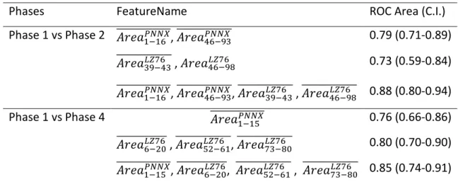
Table 4. ROC Area and confidence interval obtained using pNNx, LZ16 and their combination in differentiating phases (Phase 1 vs Phase 2 and Phase 1 vs Phase 4). Multiple features were combined using a linear regression model.
Phases FeatureName ROC Area (C.I.)
Phase 1 vs Phase 2 𝐴𝑟𝑒𝑎̅̅̅̅̅̅̅̅̅̅̅̅̅, 𝐴𝑟𝑒𝑎1−16𝑃𝑁𝑁𝑋 46−93 𝑃𝑁𝑁𝑋 ̅̅̅̅̅̅̅̅̅̅̅̅̅ 0.79 (0.71-0.89) 𝐴𝑟𝑒𝑎39−43𝐿𝑍76 ̅̅̅̅̅̅̅̅̅̅̅̅̅ , 𝐴𝑟𝑒𝑎46−98𝐿𝑍76 0.73 (0.59-0.84) 𝐴𝑟𝑒𝑎1−16𝑃𝑁𝑁𝑋 ̅̅̅̅̅̅̅̅̅̅̅̅̅, 𝐴𝑟𝑒𝑎̅̅̅̅̅̅̅̅̅̅̅̅̅, 𝐴𝑟𝑒𝑎46−93𝑃𝑁𝑁𝑋 39−43𝐿𝑍76 ̅̅̅̅̅̅̅̅̅̅̅̅̅ , 𝐴𝑟𝑒𝑎̅̅̅̅̅̅̅̅̅̅̅̅̅ 0.88 (0.80-0.94) 46−98𝐿𝑍76 Phase 1 vs Phase 4 𝐴𝑟𝑒𝑎̅̅̅̅̅̅̅̅̅̅̅̅̅ 1−15𝑃𝑁𝑁𝑋 0.76 (0.66-0.86) 𝐴𝑟𝑒𝑎6−20𝐿𝑍76 ̅̅̅̅̅̅̅̅̅̅̅̅ , 𝐴𝑟𝑒𝑎̅̅̅̅̅̅̅̅̅̅̅̅̅, 𝐴𝑟𝑒𝑎52−61𝐿𝑍76 73−80 𝐿𝑍76 ̅̅̅̅̅̅̅̅̅̅̅̅̅ 0.80 (0.70-0.90) 𝐴𝑟𝑒𝑎1−15𝑃𝑁𝑁𝑋 ̅̅̅̅̅̅̅̅̅̅̅̅̅, 𝐴𝑟𝑒𝑎̅̅̅̅̅̅̅̅̅̅̅̅, 𝐴𝑟𝑒𝑎6−20𝐿𝑍76 52−61𝐿𝑍76 ̅̅̅̅̅̅̅̅̅̅̅̅̅ , 𝐴𝑟𝑒𝑎̅̅̅̅̅̅̅̅̅̅̅̅̅ 0.85 (0.74-0.91) 73−80𝐿𝑍76 𝐴𝑟𝑒𝑎1−16𝑃𝑁𝑁𝑋
̅̅̅̅̅̅̅̅̅̅̅̅̅ represents the average area of pNNx feature profile, where 𝑥 ∈ [1,16] . This range was calculated based on sequences of x for which the ROC area is greater than 12.
FIGURES
Figure 1: The distributions of mean pNNx values within each phase of the experiment for
NN=[1,100]
Phase 1 – first resting phase, Phase 2 – dummy stimulation phase, Phase 3 – second resting
Figure 2: The distributions of mean LZ76 within each phase of the experiment for NN=[1,100]
Phase 1 – first resting phase, Phase 2 – dummy stimulation phase, Phase 3 – second resting
Figure 3: ROC Area of pNNX feature for differentiating Phase 1 from Phase 2 and Phase1
Figure 4: ROC Area of LZ76 feature for differentiating Phase 1 from Phase 2 and Phase1 from
![Figure 1: The distributions of mean pNNx values within each phase of the experiment for NN=[1,100]](https://thumb-eu.123doks.com/thumbv2/123doknet/13177135.390963/28.892.127.833.257.723/figure-distributions-mean-pnnx-values-phase-experiment-nn.webp)
![Figure 2: The distributions of mean LZ76 within each phase of the experiment for NN=[1,100]](https://thumb-eu.123doks.com/thumbv2/123doknet/13177135.390963/29.892.169.728.224.536/figure-distributions-mean-lz-phase-experiment-nn.webp)