Dynamic Reconfiguration of Feature Models: an Algorithm and its Evaluation

HAL Id: hal-01392796

https://hal.inria.fr/hal-01392796

Submitted on 4 Nov 2016

HAL is a multi-disciplinary open access

archive for the deposit and dissemination of

sci-entific research documents, whether they are

pub-lished or not. The documents may come from

teaching and research institutions in France or

abroad, or from public or private research centers.

L’archive ouverte pluridisciplinaire HAL, est

destinée au dépôt et à la diffusion de documents

scientifiques de niveau recherche, publiés ou non,

émanant des établissements d’enseignement et de

recherche français ou étrangers, des laboratoires

publics ou privés.

Dynamic Reconfiguration of Feature Models: an

Algorithm and its Evaluation

Sabine Moisan, Jean-Paul Rigault

To cite this version:

Sabine Moisan, Jean-Paul Rigault. Dynamic Reconfiguration of Feature Models: an Algorithm and

its Evaluation. [Research Report] RR-8972, INRIA Sophia Antipolis. 2016, pp.16. �hal-01392796�

0249-6399 ISRN INRIA/RR--8972--FR+ENG

RESEARCH

REPORT

N° 8972

of Feature Models: an

Algorithm and its

Evaluation

RESEARCH CENTRE

SOPHIA ANTIPOLIS – MÉDITERRANÉE

Sabine Moisan, Jean-Paul Rigault

Project-Teams Stars

Research Report n° 8972 — November 2016 — 16 pages

Abstract: This paper deals with dynamic adaption of software architecture in response to context changes. In the line of “models at run time”, we keep a model of the system and its context in parallel with the running system itself. We adopted an enriched Feature Model approach to express the variability of the architecture as well as of the context. A context change is transformed into a set of feature modifications (selection/deselection) that we validate against the feature model to yield a new suitable and valid architecture configuration. Then we update the model view of the configuration and the running system architecture accordingly. The paper focuses on the feature model reconfiguration step and details the algorithms and heuristics that implement our adaptation rules. The approach is illustrated with a simple example borrowed from the video-surveillance domain. The efficiency of the algorithm is evaluated on randomly generated feature models (from 60 to 1400 features). Our results show that in our target applications (video analysis), the processing time of a context change may be considered negligible.

Un algorithme de reconfiguration dynamique des modèles

de “features” et son évaluation

Résumé : Cet article concerne l’adaptation dynamique d’une architecture logicielle en réponse à des changements du contexte d’exécution. Dans la lignée de “models at run time”, nous conser-vons lors de l’exécution du système un modèle de ce système et de son contexte. Nous aconser-vons adopté un formalisme enrichi de modèle de “features” pour exprimer la variablité de l’architecture aussi bien que du contexte. Un changement de contexte est transformé en un ensemble de modi-fications (sélection ou désélection) de “features”; nous vérifions la consistence de ces modification par rapport au modèle pour générer une nouvelle configuration valide et adaptée au nouveau contexte. Ensuite nous modifions le modèle de la configuration courante et l’architecture du système qui en est la réalisation. L’article se concentre sur l’étape de reconfiguration du modèle de “features” et détaille les algorithmes et les heuristiques utilisés. Nous illustrons notre ap-proche avec un exemple simple emprunté au domaine de la vidéo-surveillance. Les performances de notre algorithmes sont évalués à partir de modèles de “features” générés aléatoirement (de 60 à 1400 “features”). Les résultats montrent que pour nos applications en analyse de vidéo, le temps de calcul pour prendre en compte un changement de contexte peut être considéré comme négligeable.

1

Introduction

We experiment with video understanding systems that are critical applications, running in real-time, possibly 24 hours a day, and with high dependability requirements. Moreover, they are sensitive to context variations such as lighting conditions, indoor/outdoor situation, scene com-position evolution, or noise. Therefore, these software systems must be self-adaptive, i.e. able to modify their run-time configuration according to context changes. To this end we adopted the “model at run-time” approach, meaning that in parallel with the running system, we keep its model and use the latter to drive the reconfigurations. We also keep a view that reflects the current architectural configuration of the system. The objective is to always have a running system which is correct with respect to its model and well-suited to its execution context. In our case, we use enriched feature modeling to express the variability of the architecture as well as of the context.

Our ultimate goal is to control the system through a feed back loop from video components and sensor events to feature model manipulation and back to video components modifications. The complete structure of our system is described in [8]. Briefly speaking, context changes are detected by system sensors then translated into feature modification requests. Applying these modifications produces a valid sub-model suited to the new context. The next phase is to automatically extract an appropriate configuration from this sub-model. If one is found, the last step is to update both the current configuration view and the running system architecture accordingly. The present paper only details the algorithm and the heuristics to produce a valid sub-model from feature modification requests.

Section 2 describes our model at run time: a feature model with constraints and rules. It also shows how we prepare the feature model before deployment for future context changes. Section 3 develops what happens when the context of the system changes, with a focus on adaptation rules and section 4 shows how these rules apply on a small realistic example in video surveillance. In section 5 we present some performance evaluations. Finally section 6 compares this work with similar approaches.

2

Run Time Model

2.1

Feature Model Representation

Feature Models (FM) [3,11] allow a designer to represent all possible run-time configurations of a system and provide a compact formalism to model software commonalities and variabilities. In this approach, “features” correspond to selectable concepts of a software system and of its contextual environment. They are organized along a tree, with logical selection relations (op-tional/mandatory features, exclusive choices...). Moreover, since features are not independent, one usually adds cross tree constraints to express relationships between features. In our case, we added constraints in the form of simple first order logic formulas of two types: imply noted ⇒ and exclude noted ⊗: a feature may either imply or exclude another one.

To cope with reconfiguration needs, we have enriched the feature model formalism. Among the regular extensions, besides cross tree constraints, we introduced default choices in alternatives (ors and xors). We also added less usual extensions such as states and labels (introduced in sec-tion 2.2), and quality attributes and metrics to facilitate the search for an optimal configurasec-tion (these latter are not in the scope of this paper).

We use a classical and normalized form of feature model. A model has a single root feature. A feature can be related to children features through hyperlinks of different types: and, xor, or. A hyperlink is composed of several links to children features, down to leaf features. Links can

4 S. Moisan & J.-P. Rigault

be mandatory (default) or optional (the latter is meaningful only in and hyperlinks). Figure 1 presents an example of such a model.

Applica'on* ObjectOfInterest* Acquisi'on* _{Classifica'on*}

Intrusion*

With*Reco* Without*_Reco*

Face* Recogni'on* * Color* B&W* NearIR* FullColor* ICVS*2011* Person* Detec'on* * AnyObject* Detec'on* * * * * mandatory* op'onal* OR*group* XOR*group* AND*group* implies* excludes* X* Default*Selec'on* Feature'model'seman.cs' Cross1tree'constraints'

Coun'ng* Any** People **

VS'System'

ContextView' Implementa.onView'

X*

permanent*feature*

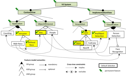
Figure 1: Initial configuration: detection of any intrusion. The permanent features (mandatory in all configurations) are marked with a (green) pin. The selected features are represented with a “tick”.

A valid configuration (i.e., combination of features) is obtained by selecting features respect-ing the Feature Model semantics. The cross tree constraints further restrict the valid combina-tions of features.

While feature models are classically used to assist system configuration before deployment, our original approach is to exploit them at run time for dynamic adaptation [7].

2.2

Dynamic Adaptation Extensions

The inputs for dynamic adaptation are merely selections or deselections of features. They come from upstream “adaptation rules” that map context changes onto feature modification requests. The role of dynamic adaptation is to apply these modifications to the model view of the current configuration under the control of the feature model. As already mentioned, the output is not in general a full configuration but rather a sub-model (a set of valid configurations).

To implement the dynamic adaptation algorithm we made several extensions to the usual Feature Model representation.

First, we extended the choice hyperlinks with the notion of a default selection when no other information is available: in the case of xor, the designer can select only one child as default whereas, in an or there may be several children selected by default. For optional links, the default is deselected.

Second, we introduced the two important notions of state and label for features.

The state of a feature corresponds to its status in the current configuration. At a given time, a feature can be in one of the following states: selected(the feature belongs to the current

configuration), deselected (the feature does not belong to the current configuration), orunknown

(the feature is undetermined, and could belong to the current configuration or not, depending on further selections/deselections). We denote [f] the state of the feature f.

The label of a feature corresponds to the possibility to change its state during reconfiguration, depending on the context. This label can be either permanent (the state cannot be changed in

any context),required(the state cannot be changed in the current context, because it is required

by the context change),deduced (the state cannot be changed in the current context, because it

is a mandatory consequence of a feature labeled required), or mutable(the state can be changed).

We denote ¯f the label of the feature f.

When deploying the system, as well as at the end of a dynamic configuration change (when an optimum valid configuration has been found and applied), we change the labels of all non permanent features tomutable for future context changes.

2.3

Definition of the Core Model

The core model is the one that we keep at run time. It can be a sub-model of a bigger model but it targets the system application: it contains all the features necessary for all use cases of the application and only them. Thus the unneeded features are eliminated. From this core, we shall deduce the adapted run time configuration at each context change. We define this model off line, before deploying the system.

We start by identifying and labeling the features that cannot change their state (they must

beselectedin any context), otherwise the FM would become invalid. The root of the FM must be

selected at least. If the root has an and hyperlink to its children, the mandatory root’s children should be selected too, and so on. The state of these features is set to selected and they are

labeled as permanent.

So the core model is a FM with some features (at least the root)selectedand labeledpermanent

and all the others in stateunknownand labeled mutable. During the evolution of the system, the

states and labels of features will change.

3

Context Change Algorithm

The goal of run time adaptation is to ensure that, at any time, the running system conforms to the core model and is well-suited to its execution context. The rest of the paper details our algorithm to obtain a new valid sub-model.

3.1

Rationale and Overview

The algorithm is triggered by each context change, expressed as a list of features to select or deselect in the feature model. Then it computes in real time a valid sub-model for the new context. It relies only on the core model, the current running configuration, and the context related feature selections/deselections. The execution time of the algorithm should be short enough to be compatible with the context change frequency as well as with the load induced by system main operation, in our case video analysis, a rather heavy duty processing. The context changes that we address follow the rhythm of human activities.

Basically, the algorithm tries to find local modifications for the parts of the feature model that contain a changed feature (to be either selected or deselected). The aim is to make the minimum number of modifications to the current configuration, yet leading to a valid feature sub-model.

6 S. Moisan & J.-P. Rigault

3.2

Initial Step

At each context change, the adaptation rules provide us with a set S of features that must be selected due to the change, and a set D of features that must be deselected. We first check the consistency of these sets:

• Apply constraints (imply and exclude) related to features in both sets; this extends S and D with the features that are implied or excluded by the presence/absence of features in original S and D. Complete S and D with the transitive closure of all constraints to obtain the “minimal” sets of features the state of which should beselected(resp. deselected).

• Then test that the intersection of extended S and D is empty. Otherwise stop, since it would not be possible to find any valid configuration (and do not change the running one).

3.3

Find a Valid Sub-Model

If the previous initial step succeeds, the second step is to find all the new valid configurations of the system, which comes down to find a sub-model of the core model, where all the configurations are valid in the new context.

We start from the currently applied configuration (initial or run time one), the idea is to derive a sub-model from it, with minimum modifications. In this configuration the labels of all non permanent features aremutable(see 2.2) and their state is the one set in the running system.

In the current configuration, for all features in S ∪ D, we first change their state if necessary (if the feature is already in the desired state, there is nothing to do) and we label them asrequired

in this context (unless they arepermanent).

∀fi∈ S(resp. D) {

if ( ¯fi= permanent ∧ fi∈ S)

// permanent and deselected is stupid ! if ([fi] 6= selected) error;

¯

fi← required;

[fi] ← selected; //(resp. deselected )

}

Then, for each feature which was not previously in the desired state, we need to propagate the change to its parent and sibling features and to its children features, if any. These two steps apply the FM semantics depending on hyperlink and link types. They may assign new states to features, which will then be labeled asdeduced.

Finally, we propagate constraints only on features labeled asdeduced, since other constraints

were applied in initial step (see previous section).

3.3.1 Algorithm try_assign

The propagation to parent/siblings/children invokes a recursive Boolean function try_assign, described below, that tries to assign a state to a feature.

bool try_assign(Feature f , State desired_state) { //desired_state is selected or deselected if ([f ] = desired_state) { // just change label if needed

if ( ¯f 6=permanent) ¯ f ← deduced; return true; // ok } Inria

// f is not in desired state

if ( ¯f 6= mutable) // state of f cannot be changed return false; // error

// else state of f can be changed, let ’ s try [f ] ← desired_state;

¯

f ← deduced;

if (¬ propagate_parent_siblings(f,desired_state)) return false;

if (¬ propagate_children(f,desired_state)) return false; if (¬ propagate_constraints(f,desired_state)) return false; return true;

}

3.3.2 Propagation of state change to other features

Considering a feature f, we denote p its parent, {s1..sn}its siblings, and {c1..cm} its children,

if any.

We summarize the algorithms of propagation of state change to parent, siblings, and children in three tables (1 to 3). These algorithms rely on the semantics of feature diagrams and on a few heuristics based on our extensions or on logic properties. They can return ok (the sub-model is valid so far), error (no valid sub-model is possible), or undefined (no consistent changes can be performed, due to lack of information). In the two last cases the running configuration is unchanged.

Table 1 describes the propagation of changes towards parents and siblings. Note that or and xor processing are the same except for parent’s default selection. Table 2 shows how a feature state change propagates to its children. Table 3 describes the propagation of cross tree constraints. Our constraints are of the form f ⇒ f1 (imply) or f ⊗ f1 (exclude). They have

only one feature in the left part and one in the right part. To express conjunctions, we can write several constraints: f ⇒ f1∧ f2 is written as f ⇒ f1 and f ⇒ f2. Similarly, to express

disjunctions we replace f1∨ f2 ⇒ f with f1 ⇒ f and f2 ⇒ f. Currently, we do not support

conjunction in the left part nor disjunction in the right part of an implication.

Note that these algorithms do not in general find a unique adapted configuration but rather a sub-model (that is several adapted valid configurations). To extract one of those, we developed an optimal search procedure using an utility function based on feature quality attributes [10].

4

Example

The domain of video surveillance offers an ideal training ground for our studies on dynamic adaptation. Indeed, video surveillance systems should run in real-time, possibly 24 hours a day, in various situations. They hence require run time adaptation of their architecture to react to changing conditions in their context of execution.

As a matter of example, consider a simple intrusion detection application with optional person recognition. The initial scene is empty and should remain empty except for temporary presence of a few authorized persons. Initially the system is set to a “low cost” intrusion detection mode without recognition (only movement is detected). Thus in the feature model of figure 1 features

Intrusionand WithoutRecoare selected. For the two xors associated withObjectOfInterest andColor,

default selection applies: thereforeAnyandB&Ware chosen.

When an intrusion occurs, the eventIntrusionDetectedis generated and triggers an adaptation

8 S. Moisan & J.-P. Rigault

Table 1: Propagation to parent and siblings

[f ] ← selected [f ] ← deselected and(p) try_assign(p,selected) if (f optional) ok

else try_assign(p,deselected)1 xor(p) try_assign(p,selected) case [p]deselected: ok (at this level)

∀sj6= f case [p]selected:

try_assign(sj,deselected) if (∃!o/[so]=selected) ok

if (∀l ∈ {1..n}[sl] 6=selected)2

if (∃!k/[sk]=unknown) try_assign(sk,selected)

else if (∃!k/ ¯sk=mutable) try_assign(sk,selected)

else if (n=2) try_assign(sj,selected)/sj6= f

else if (∃!sd=p.default_selection) try_assign(sd,selected)

case [p]unknown:

if (∀l ∈ {1..n}[sl]=deselected) try_assign(p,deselected)

if (¯p=mutableand ∀l ∈ {1..n}[sl]=deselected)

try_assign(p,deselected)

or(p) try_assign(p,selected) case [p]deselected_{: ok (at this level)}

case [p]selected:

if (∃o/[so] =selected) ok

if (∀l ∈ {1..n}[sl] 6=selected)

if (∃!k/[sk]=unknown) try_assign(sk,selected)

else if (∃!k/ ¯sk=mutable) try_assign(sk,selected)

else if (n=2) try_assign(sj,selected)/sj6= f

else ∀sd=p.default_selection try_assign(sd,selected)

case [p]unknown:

if (∀l ∈ {1..n}[sl]=deselected) try_assign(p,deselected)

if (¯p=mutableand ∀l ∈ {1..n}[sl]=deselected)

try_assign(p,deselected)

Note1: applying try_assign to parent p will propagate changes to the siblings of f .

Note2_{: the idea of this heuristics is to prioritize the choice of sibling to select when the parent of f}

is selected. First, if there is a unique sibling which has no state (its state isunknown), try to select it as first choice. Otherwise if it exists a single sibling whose state can be changed (labeledmutable), try to select it as second choice. Thirdly, in the particular case of a xor with only 2 children, f being deselected, the other child must be selected to comply with xor semantics. Lastly, we try to select the default selection of the parent xor, if any. In all other cases, there is not enough information to deduce any meaningful propagation and the output of the algorithm is undefined.

Table 2: Propagation to children

[f]←selected [f]←deselected

and(f) ∀j ∈ 1..m

∀j ∈ {1..m} if (cj not optional) try_assign(cj,selected)

try_assign(cj,deselected)

xor(f)

if (∀j ∈ {1..m}[cj] 6=selected)

if (∃!k/[ck]=unknown) try_assign(ck,selected)

else if (∃!k/ ¯ck=mutable)try_assign(ck,selected)

or(f)3 _{else if (∀j[c}

j]=deselected) error

Note3: Concerning children, propagation in ORs and xors is completely equivalent.

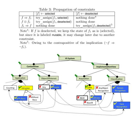
Table 3: Propagation of constraints

[f ] ←selected [f ] ←deselected

f ⇒ f1 try_assign(f1,selected) nothing done4

f ⊗ f1 try_assign(f1,deselected) nothing done

f1⇒ f nothing done try_assign(f1,deselected)5

Note4: If f is deselected, we keep the state of f1 as is (selected),

but since it is labeledmutable, it may change later due to another constraint.

Note5: Owing to the contrapositive of the implication (¬f ⇒ ¬f1).

Intrusion*

With*Reco* Without*_Reco*

Face* Recogni'on* * Color* B&W* NearIR* FullColor* Person* Recogni'on* * AnyObject* Recogni'on* * * * * * * * * * Coun'ng* X* Any* People* ** *

Applica'on* ObjectOfInterest* Acquisi'on* Classifica'on*

VS'System'

ContextView' Implementa.onView'

Figure 2: Adapted configuration after detected intrusion. Newly selected features (S) are repre-sented in gray/blue with a “tick”, and the ones to be deselected (D) with a red “cross”.

additional face recognition algorithm, to identify the intruder and possibly check whether the person is authorized or not (and raise an alarm if not). Therefore the set of features to be selected is S = {WithReco}and the set to be deselected is D = ∅.

We then run the initial step (section 3.2) applying the cross tree constraints. Following figure 1, the cross tree constraints

WithReco⇒People,WithReco⇒FaceDetection,People⇒PersonDetection,FaceDetection⇒FullColor

lead to

S = {FaceDetection,FullColor,PersonDetection,WithReco,People} It is still true that S ∩ D = ∅. The final result is depicted on figure 2.

To find a valid sub-model (section 3.3) we now enforce FM semantics. Here the xor nodes impose to deselectWithoutRecoon the one hand and all the other variants ofColor(B&WandNearIR)

on the other hand. Consequently we add {WithoutReco,B&W,NearIR,Any,AnyObjectRecognition}to D.

Since the added features have no unsatisfied associated cross-constraints, the propagation stops. Here the result is not a sub-model but a unique configuration. The configuration delta, i.e. the current contents of S and D will be transformed into software architecture changes (addition, removal, replacement of components, parameter tuning...).

10 S. Moisan & J.-P. Rigault

5

Analysis and Experiments

With such an algorithm, one may fear multiple traversals of feature (sub-)trees, hence an explo-sion of the processing time. In our experience, we were never confronted with such a drawback. To reinforce this feeling, we conducted two types of empirical experiments. The first experiment is a brute force measure of the time to apply large sets of selections and deselections (S and D) to randomly generated feature models of various size. In the second experiment, we choose a reasonable size model (280 features) and we measure the time to process a single simple change in different cases.

All measures were performed under Fedora Linux 19 (64 bits) running on Intel® _Xeon®

processor at 2.10GHz with 32Mbytes of memory. The program is written in C++. Processor times are measured using the high resolution clock of the C++ std::chrono library.

5.1

Multiple Selections and Deselections

After fixing thepermanent features to obtain the core model that will be kept at run time

(sec-tion 2.3), the second step is to specialize this core model for the target applica(sec-tion. Usually, it is the role of the user to select or deselect the suitable features at deployment time. It comes down to applying our algorithm (section 3.3) with large S and D sets. In general, the size of these sets is much bigger than expected during regular context changes when the application runs. Therefore it seems meaningful to measure the time necessary for this second step against the size of the model.

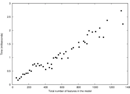
We randomly generated feature models based on three parameters: the total number of features (from 60 to 1400), the number of hyperlinks expressed as a percentage of the former (currently 10%), and the distribution of hyperlink types (currently 50% ands, 25% ors and 25% xors. We added a few (0 to 5) cross tree constraints. With these parameters, the resulting feature trees exhibit a branching factor from 3 to 6 and a number of levels from 3 to 6.

For each generated model we randomly created one S and one D set. The size of these sets (cardinality of S ∪ D) grows with the model size (from 8 to 60 features). The results are shown on figure 3. Each point on this graph represents the average of ten identical runs. No processing time explosion is noticeable. In fact the time seems to grow rather linearly. Moreover, the computation time of a new initial sub-model does not exceed 3 ms for a rather big model.

5.2

Unitary Context Changes

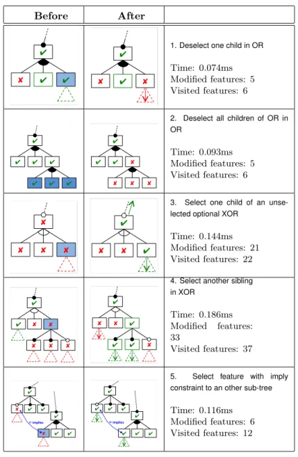
This second test uses one fixed feature model with 280 features (generated as mentioned before). We perform on this tree a series of changes, each one selecting or deselecting feature(s) corre-sponding to simple changes to the model. Indeed, in practice a context change leads to a few such feature modifications, hence the interest to measure the time to propagate the impact of such “unitary” changes. In table 4 we present some typical changes. The indicated times are the average of half a dozen identical runs.

In the table, the left column sketches the situation before the change. The features marked in grey are those that are explicitly referred in the adaption rule; hence changing their state is the starting point of the algorithm. Potential children sub-trees are indicated by dotted triangles. The middle column shows the situation after the effects of the change have been propagated. The arrows indicate a propagation upwards to the parent or downwards to the children. In the rightmost column, besides the average processing time, we show the number of features the state of which has changed (Modified features) and the total number of features visited by the algorithm (Visited features). The last test (number 5) is an attempt to evaluate the effect of

Table 4: Cost of some unitary context changes Before After * * * * * * * * Test*5* Deselect*one*child*in*OR* * * * * * * * * Test*5* Deselect*one*child*in*OR*

1. Deselect one child in OR

Time: 0.074ms Modified features: 5 Visited features: 6 * * * * * * * * * * * * * * * * * * * * * * * * * Test*2* Deselect*all*children*of*an*OR* Test*1* Select*one*child*of** unselected*op'onal*XOR* * * * * * * * * * * * * * * * * * * * * * * * * * Test*2* Deselect*all*children*of*an*OR* Test*1* Select*one*child*of** unselected*op'onal*XOR*

2. Deselect all children of OR in OR Time: 0.093ms Modified features: 5 Visited features: 6 * * * * * * * * * * * * * * * * * * * * * * * * * Test*2* Deselect*all*children*of*an*OR* Test*1* Select*one*child*of** unselected*op'onal*XOR* * * * * * * * * * * * * * * * * * * * * * * * * * Test*2* Deselect*all*children*of*an*OR* Test*1* Select*one*child*of** unselected*op'onal*XOR*

3. Select one child of an unse-lected optional XOR

Time: 0.144ms Modified features: 21 Visited features: 22 * * * * * * * * * * * * * * Test*3* Select*an*other*sibling*in*XOR* Test*4* Select*an*unrelated*feature*with*constraint** to*another*op'onal*subtree* * * * * * * * * 'implies' * * * * * * * * 'implies' * * * * * * * * * * * * * * Test*3*_{Select*an*other*sibling*in*XOR*} Test*4* Select*an*unrelated*feature*with*constraint** to*another*op'onal*subtree* * * * * * * * * 'implies' * * * * * * * * 'implies'

4. Select another sibling in XOR Time: 0.186ms Modified features: 33 Visited features: 37 * * * * * * * * * * * * * * Test*3* Select*an*other*sibling*in*XOR* Test*4* Select*an*unrelated*feature*with*constraint** to*another*op'onal*subtree* * * * * * * * * 'implies' * * * * * * * * 'implies' * * * * * * * * * * * * * * Test*3*_{Select*an*other*sibling*in*XOR*} Test*4* Select*an*unrelated*feature*with*constraint** to*another*op'onal*subtree* * * * * * * * * 'implies' * * * * * * * * 'implies'

5. Select feature with imply constraint to an other sub-tree

Time: 0.116ms Modified features: 6 Visited features: 12

12 S. Moisan & J.-P. Rigault

Figure 3: Computation time of initial models

cross tree constraints. Here an imply constraint was manually inserted to relate two remote sub-trees.

The results show that the processing time for a unitary change is short, especially when compared with the period of context changes that we experiment in our video-surveillance appli-cations. Indeed, the impact of a context change usually remains local: in our tests, the number of visited levels in the tree does not exceed 3. Moreover, the number of visited features is not much superior to the number of the changed ones. This indicates that the algorithm is parsi-monious when visiting the tree: it visits no more nodes than required. The only exception to locality is due to cross tree constraints: in case of many of those, the number of required visits might increase. This is unavoidable but, on the other hand, a model with really many cross tree constrains becomes humanly intractable.

However, since the result of our algorithm is only a valid sub-model, one has then to extract a specific configuration. We address this configuration problem, which usually takes much more time, in an other work [10].

6

Related Works

We are in the line of Models at Run-Time as described, for instance, in [4] which considers context aware systems that maintain “run time models reflecting the running system and its environment” and where the models are the “primary drivers of the adaptation”. In our case, on figure 1 the core model is kept at run time and it distinguishes clearly the environment (children of feature ContextView) from the running system representation (children of feature

ImplementationView). Moreover, any configuration change has to comply with this model.

Feature model processing tends to increase exponentially. To avoid overwhelming compu-tation at run time, several authors use offline preprocessing of their variability models. For instance, [9] statically merge features that are used together in the application scenarios into “binding units”. This allows them to reduce the variability to be handled at run time and thus

the computation cost. Another approach is to list at design time all the possible context changes and to check statically that there exists a valid configuration for each case [2]. This alleviates run time verification. Such preprocessing approaches are fine to cope with macroscopic con-text changes (switch between different modes of functioning) whereas we consider “smaller scale” changes. Moreover, our fully dynamic approach may allow emergent behaviors (valid answers to unexpected situations). Of course it may also fail to find a valid solution, in this case we keep the current configuration unchanged (and notify the users) which in our kind of target systems is usually a lesser evil.

Indeed, in the literature there are not a lot of works that address full real time local modifi-cations of FMs. In our case, at design time the users establish the core model that contains only the features relevant for the target application. This model is statically verified and the perma-nent features are automatically identified. By definition these features are fixed and thus do not contribute to the variability. At run time, when the context changes, our algorithms search for a new adapted sub-model and check it at the same time. Although the risk of explosion exists, in practice it generally appears to be tractable (see section 5).

When determining an adapted valid configuration, some systems use a goal-oriented approach, minimizing a utility function [6]. Others define rules, also called “resolutions” relating context changes and feature selection/deselection [2,5]. In fact we use both methods. First, as explained in section 3.3, adaption rules similar to resolutions lead to a valid adapted sub-model. To extract one single optimal configuration from this model we perform goal satisfaction by minimizing a weighted function of quality attributes depending on the application [10].

In some works, the context is described with a specific representation [2]. We preferred feature models for both the context and the implementation views, as shown on figure 1. This respects the separation of concerns while facilitating communication, transformation, and expression of constraints between context features and implementation ones.

Models at run time require some dedicated tools to transform and check variability models. Most authors use existing model managers usually involving SAT solvers. For instance, [5] relies on FAMA, [9] uses FeatureC++, and [2] EMF Model Query. We tried this approach in the past [1] but we realized that we had to pay for language heterogeneity (most existing tools are in Java whereas all our code is in C++ for efficiency), communication overhead, and model format transformations. Moreover third party tools do not support our feature model extensions (state, label, default selection, metrics and quality attributes) which are of primary importance for adaption. Thus we developed our own C++ feature model manipulation code which intergrates nicely into the rest of our system.

7

Conclusion and Future Work

We have presented a feature model based technique to support dynamic reconfiguration of soft-ware systems exhibiting context-sensitive variability. A context change is translated into a set of selections and deselections of features that is confronted with the model (kept at run time). The result is a new sub-model, a set of possible configurations, that is, by construction, valid with respect to the run time model. The paper details the algorithms and heuristics to obtain this adapted sub-model. Note that this is only the first step of the reconfiguration. The second step is to extract from the resulting sub-model the unique new running configuration (preferably “optimal”). This has been the topic of another work.

At run time, we keep a core model that contains all the features related to the target appli-cation. This core model represents the features related to the implementation (software compo-nents, tunable parameters) as well as the information about the context (illumination changes,

14 S. Moisan & J.-P. Rigault

scene contents evolution). This uniform representation facilitates the communication and trans-formation between the two aspects.

To allow for the reconfiguration process, we propose an enriched feature model introducing feature states and labels, and the notion of permanent features (features that are present in any configuration). Distinguishing permanent features from variable ones reduces the risk of time explosion at run time. Moreover, from our experience with video systems, the reconfigura-tion computareconfigura-tion time is negligible with respect to the execureconfigura-tion time of the vision and image algorithms.

We do not use third party tools to manipulate and check the models. We prefer to reduce communication and data format translations between the different parts of the system. Conse-quently, the feature model representation and the verification of the model are coded in the same language as the rest of the system (video components definition and operations, context change handling...), namely C++.

Beyond computation time, the real difficulty is that there might be context changes for which no solution can be found. This can be due to events leading to feature selection conflicts or to insufficient information (as mentioned in section 3.3.2). Currently we keep the current configuration as it was before the change.

As an example of the first problem, imagine that an intrusion is detected and, at the same time, the light is dimming: intrusion requires face recognition in color, whereas light dimming excludes the use of color. Finding a solution to this kind of situation is tricky. We can think of a priority mechanism but these priorities would introduce a new type of relations (neither imply nor exclude) that would link features in the context view sub-tree.

In the near future we plan to tackle the second problem by enriching the feature model with additional information such as priorities to choose between children in or and xor hyperlinks and supplementary rules (sort of “weak” constraints) to decide upon selection of optional features.

References

[1] Mathieu Acher, Philippe Collet, Philippe Lahire, Sabine Moisan, and Jean-Paul Rigault. Modeling variability from requirements to runtime. In 16th IEEE International Conference on Engineering of Complex Computer Systems, ICECCS 2011, Las Vegas, Nevada, USA, 27-29 April 2011, pages 77–86, 2011.

[2] Germán H. Alférez, Vicente Pelechano, Raúl Mazo, Camille Salinesi, and Daniel Diaz. Dy-namic adaptation of service compositions with variability models. Journal of Systems and Software, 91:24–47, 2014.

[3] Don S. Batory. Feature models, grammars, and propositional formulas. In SPLC’05, pages 7–20, 2005.

[4] Amel Bennaceur, Robert France, Giordano Tamburrelli, Thomas Vogel, Pieter J. Moster-man, Walter Cazzola, Fabio M. Costa, Alfonso Pierantonio, Matthias Tichy, Mehmet Akşit, Pär Emmanuelson, Huang Gang, Nikolaos Georgantas, and David Redlich. Models@Run-Time, volume 8378 of LNCS, chapter Mechanisms for Leveraging Models at Runtime in Self-Adaptive Software, pages 19–46. Springer, 2014.

[5] Carlos Cetina, Pau Giner, Joan Fons, and Vicente Pelechano. Autonomic computing through reuse of variability models at runtime: The case of smart homes. IEEE Computer, 42(10):37– 43, 2009.

[6] Naeem Esfahani, Ahmed M. Elkhodary, and Sam Malek. A learning-based framework for engineering feature-oriented self-adaptive software systems. IEEE Trans. Software Eng., 39(11):1467–1493, 2013.

[7] S. Moisan, J.-P. Rigault, and M. Acher. A feature-based approach to system deployment and adaptation. In ICSE Workshop on Modeling in Software Engineering (MISE), pages 84–90, Zurich, Switzerland, June 2012.

[8] Sabine Moisan, Jean-Paul Rigault, Mathieu Acher, Philippe Collet, and Philippe Lahire. Run time adaptation of video-surveillance systems: A software modeling approach. In Computer Vision Systems - 8th International Conference, ICVS 2011, Sophia Antipolis, France, September 20-22, 2011. Proceedings, pages 203–212, 2011.

[9] Marko Rosenmüller, Norbert Siegmund, Mario Pukall, and Sven Apel. Tailoring dynamic software product lines. In Generative Programming And Component Engineering, Pro-ceedings of the 10th International Conference on Generative Programming and Component Engineering, GPCE 2011, Portland, Oregon, USA, October 22-24, 2011, pages 3–12, 2011. [10] Luis Emiliano Sanchez, J. Andres Diaz-Pace, Alejandro Zunino, Sabine Moisan, and Jean-Paul Rigault. An approach based on feature models and quality criteria for adapting component-based systems. Journal of Software Engineering Research and Development (JSERD), 3(10), June 2015.

[11] Pierre-Yves Schobbens, Patrick Heymans, Jean-Christophe Trigaux, and Yves Bontemps. Generic semantics of feature diagrams. Comput. Netw., 51(2):456–479, 2007.

16 S. Moisan & J.-P. Rigault

Contents

1 Introduction 3

2 Run Time Model 3

2.1 Feature Model Representation . . . 3

2.2 Dynamic Adaptation Extensions . . . 4

2.3 Definition of the Core Model . . . 5

3 Context Change Algorithm 5 3.1 Rationale and Overview . . . 5

3.2 Initial Step . . . 6

3.3 Find a Valid Sub-Model . . . 6

3.3.1 Algorithm try_assign . . . 6

3.3.2 Propagation of state change to other features . . . 7

4 Example 7 5 Analysis and Experiments 10 5.1 Multiple Selections and Deselections . . . 10

5.2 Unitary Context Changes . . . 10

6 Related Works 12

7 Conclusion and Future Work 13