HAL Id: hal-01087222
https://hal.archives-ouvertes.fr/hal-01087222
Submitted on 26 Nov 2014
HAL is a multi-disciplinary open access
archive for the deposit and dissemination of
sci-entific research documents, whether they are
pub-lished or not. The documents may come from
teaching and research institutions in France or
abroad, or from public or private research centers.
L’archive ouverte pluridisciplinaire HAL, est
destinée au dépôt et à la diffusion de documents
scientifiques de niveau recherche, publiés ou non,
émanant des établissements d’enseignement et de
recherche français ou étrangers, des laboratoires
publics ou privés.
The two types of El-Niño and their impacts on the
length of day
O de Viron, Jean O. Dickey
To cite this version:
O de Viron, Jean O. Dickey.
The two types of El-Niño and their impacts on the length of
day.
Geophysical Research Letters, American Geophysical Union, 2014, 41, pp.3407 - 3412.
�10.1002/2014GL059948�. �hal-01087222�
The two types of El-Nino and their impacts on the Length-of-day
1
O. de Viron and J. O. Dickey
At the interannual to decadal timescale, the changes in 2
the Earth rotation rate are linked with the El-Ni˜no South-3
ern Oscillation phenomena through changes in the Atmo-4
spheric Angular Momentum. As climatic studies demon-5
strate that there were two types of El-Ni˜no events, namely 6
Eastern Pacific (EP) and Central Pacific (CP) events, we in-7
vestigate how each of them affect the Atmospheric Angular 8
Momentum. We show in particular that EP events are asso-9
ciated with stronger variations of the Atmospheric Angular 10
Momentum and length-of-day. We explain this difference 11
by the stronger pressure gradient over the major mountain 12
ranges, due to a stronger and more efficiently localized pres-13
sure dipole over the Pacific Ocean in the case of EP events. 14
1. Introduction
The Earth rotation is not constant in time; in particular, 15
the Earth rotation rate, and the associated length-of-day 16
(LOD) show fluctuations in a broad band of periods. A 17
global description of the causes at the different time scales 18
can be found in Hide and Dickey [1991]. The main cause of 19
LOD change for periods ranging from a few days to a few 20
years is the Earth atmosphere interaction. As soon as in-21
terannual fluctuations were observed in the Earth rotation 22
data, the El-Ni˜no Southern Oscillation (ENSO) was shown 23
to play a major role [Chao, 1984, 1988], as a warm – El-Ni˜no 24
– event has been shown associated with a longer day and a 25
cold – La Ni˜na – event associated with a shorter day. 26
Classical El-Ni˜no events are characterized by maximum 27
warm water anomaly in the Eastern Pacific Ocean, and re-28
ferred as the Eastern Pacific (EP) El-Ni˜no events, with Sea 29
Surface Temperature (SST) anomalies in the Nino-3 region 30
(5◦ S - 5◦ N, 150◦W to 90◦ W). Frequent occurrences of a 31
new type of El Ni˜no have been observed since the 1990s, with 32
the maximum warm SST anomaly in the Central Equatorial 33
Pacific [e.g. Latif et al., 1997], the Nino-4 region (5◦S - 5◦ 34
N, 160◦ E to 150◦ W). These are known with a variety of 35
names, Central Pacific (CP) El Ni˜no [Kao and Yu, 2009; Yu 36
and Kim, 2010], warm pool El Ni˜no [Kug et al., 2009], date-37
line El Ni˜no [Larkin and Harrison, 2005] or El Ni˜no Modoki 38
[Ashok et al., 2007]. These two ENSO types have differ-39
ent teleconnection patterns and climatic consequences [e.g. 40
Weng et al., 2009; Kim et al., 2009; Ashok and Yamagata,
41
2009; Kim et al., 2009]. In this study, we investigate how 42
the EP and CP event mechanisms affect the Earth rotation 43
differently. 44
1Universit´e Paris Diderot, Sorbonne Paris Cit´e, and
Institut de Physique du Globe de Paris (UMR7159), now at Univ La Rochelle, CNRS, UMR 7266, Littoral
Environnement & Soci´et´e LIENSs, F-17000 La Rochelle, France
2Jet Propulsion Laboratory, California Institute of
Technology, Pasadena, CA
Copyright 2014 by the American Geophysical Union. 0094-8276/14/$5.00
Classically, the atmospheric impact on the Earth rota-45
tion is estimated using the angular momentum (AM) ap-46
proach: the solid Earth+atmosphere system is considered 47
as isolated, the atmospheric angular momentum (AAM) is 48
computed, considering that any variation of this quantity 49
is compensated by an opposite variation of the Earth AM. 50
The AAM is composed of two parts, a mass term corre-51
sponding to the AM associated with the rigid rotation of 52
the atmosphere with the solid Earth, and a motion term 53
corresponding to the relative AM of the atmosphere with 54
respect to the solid Earth. 55
Alternatively, as first proposed by Widger [1949], one can 56
also consider the atmosphere as an external forcing to the 57
solid Earth. The total atmospheric torque acting on the 58
solid Earth is the sum of four effects: a pressure effect on the 59
topography, the gravitational interaction between the atmo-60
spheric and the Earth masses, the wind friction drag over the 61
Earth surface, and the interaction between the gravity wave 62
and the topography [Barnes et al., 1983; Huang et al., 1999]. 63
The last term is generally negligible [de Viron and Dehant , 64
2003]. The topography from the atmospheric Global Circu-65
lation Models (GCMs) is classically defined with respect to 66
the geoid; consequently, the topographic torque computed 67
using such a topography is actually the sum of topogra-68
phy and gravitational torque, and is known as the mountain 69
torque. The total torque is thus computed as the sum of the 70
mountain and the friction torque. 71
Generally, the mountain torque generates the axial AAM 72
variations, which are eventually damped away by the friction 73
torque [de Viron et al., 2001; Lott et al., 2008; Marcus et al., 74
2011]. A noticeable exception is the seasonal AAM anomaly, 75
which is generated by an anomalous friction torque over the 76
Indian Ocean [de Viron et al., 2002]. Both the atmospheric 77
AM (AAM) and torques can be estimated from the output, 78
whereas the inherent accuracy limits this method at the un-79
derstanding of the physical processes but does not allow to 80
estimate Earth rotation variation with a precision allowing 81
to use it in the frame of geodetic studies [de Viron and De-82
hant , 2003].
83
The torque approach was used for understanding the 84
atmospheric angular momentum anomaly associated with 85
the ENSO phenomenon [Wolf and Smith, 1987; Ponte and 86
Rosen, 1999; de Viron et al., 2001; Marcus et al., 2010].
Dur-87
ing the ENSO event, a low pressure appears in the Eastern 88
part of the Pacific Ocean, which creates a positive torque 89
over the atmosphere and consequently increases the AAM 90
and the LOD. The increased surface wind over the North-91
ern Pacific increases the friction torque, which eventually 92
cancels the AAM anomaly. 93
2. Data Preparation
In this study, we used outputs of the National Centers 94
for Environmental Prediction – National Center for Atmo-95
spheric Research (NCEP-NCAR) reanalysis [Kalnay et al., 96
1996], from 1948 to 2013. Data includes the zonal wind 97
field (as a function of time, pressure level, latitude, and lon-98
gitude), the surface pressure and East-West wind stress (as 99
a function of time, latitude, and longitude), and the model 100
orography. 101
X - 2 DE VIRON ET AL.: TWO EL-NINO AND LOD VARIATIONS
The Z component of the AAM is estimated from 102 HZmotion = a3 g ∫ 2π 0 ∫ π 0 ∫ Psurface 0 u(p, θ, λ) sin2θdp dθ dλ (1) HZmass = a4Ω g ∫ 2π 0 ∫ π 0 Psurface(θ, λ) sin3θ dθ dλ, (2) where a is the mean Earth radius, g is the mean gravity 103
acceleration, u is the zonal wind, Psurfaceis the surface
pres-104
sure, θ and λ are the colatitude and longitude, and Ω is the 105
Earth mean angular velocity. In order to be able to inves-106
tigate the space pattern of the anomaly, we also used the 107
expression of equation (1) only integrated along the longi-108
tude, corresponding to the contribution to the motion term 109
at a given latitude, pressure level, and time. 110
The axial torque are estimated from the surface pressure 111
longitude derivative and orography using 112 ΓMountainZ = a 3 ∫ 2π 0 ∫ π 0 ∂Psurface(θ, λ) ∂λ h(θ, λ) sin θ dθ dλ (3) ΓFrictionZ = −a3 ∫ 2π 0 ∫ π 0 τλsin2θ dθ dλ, (4)
where h is the orography and τλis the zonal friction drag.
The longitude derivative of the surface pressure is estimated using a using a five-point stencil [e.g. Burden and Faires, 2010]: df (x) dx i ≃ 8fi−2− fi−1+ fi+1− 8fi+2 12 ∆x (5)
The EP and CP Ni˜no index are estimated, following Ren
and Jin [2011], from the Ni˜no 3 and Ni˜no 4 index from the NOAA Climate Prediction Center, made available at the Earth System Research Laboratory website. Defining
α =
{ 2
5
0 where Nino3· Nino4< 0
NEP = Nino3− α · Nino4 (6)
NCP = Nino4− α · Nino3 (7)
To minimize the impact of the high-frequency noise in the 113
computation, the indices are smoothed by a 1-year running 114
mean. We isolate the impact of each type of events by first 115
separating the data epochs into three categories, for each 116
index, the epochs with index values above 1σ being the pos-117
itive state, with index values below−1σ being the negative 118
state, and the value in the interval [−σ, σ] being the neutral 119 state. 120 t+X = {t : NX(t) > σNX} (8) t0X = {t : −σNX ≤ NX(t)≤ σNX} (9) t−X = {t : NX(t) <−σNX} (10)
We then compute a composite anomaly by making the dif-ference between the average positive state and the average negative state.
CX(x, y) = C(t+X, x, y)− C(t−X, x, y) (11)
where X can be either EP or CP , and C(t, x, y) is the 121
dataset at time t and coordinates (x, y). 122
3. ENSO induced AAM anomaly
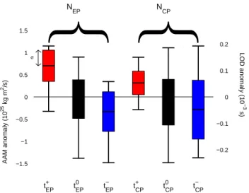
We estimated the composite impact of the ENSO by com-123
puting the mean AAM for t+,0,EP−and t+,0,CP−. Whisker dia-124
grams for each of them are plotted on Figure 1, the as-125
sociated AAM anomaly can be observed on the left axis, 126
whereas the corresponding LOD anomaly can be read on 127
the right axis. The above average values of both EP and 128
CP indices are seen to be associated with anomalously high 129
value of AAM, whereas below average index values are asso-130
ciated with anomalously low value of AAM. The difference 131
is found significant at more than 99% with an ANOVA test 132
(see Davis [1986], for example). The t0X are the largest set,
133
with about 500 epochs, whereas the + and - have about 100. 134
Due to the one-year smoothing, the epochs from the same 135
winter are not independents; consequently, for the statis-136
tics, only the mean value over a given winter was kept. The 137
ANOVA group size was subsequently of the order of 15 to 138
20 winters for the + and - epochs, and about 100 for the 0 139
epochs. 140
The EP anomaly is stronger: in particular, the difference 141
of mean between above average and below average is nearly 142
2.5 time larger for EP than for CP. 143
4. AAM and torque for the two types of
ENSO events
Such a difference in AAM signature finds its explana-144
tion in the torque acting on the atmosphere from the solid 145
Earth. As explained in Ponte and Rosen [1999], the torque 146
causing the AAM anomaly in the case of an ENSO event is 147
the mountain torque associated with the pressure anomaly. 148
The Southern Oscillation is known (see for instance Clarke 149
[2008]) to be associated with a pressure East-West dipole 150
over the Pacific. However, depending on the type of events, 151
the location of this dipole is directly linked to that of the SST 152
anomaly, as shown on Figure 2. In particular, the EP neg-153
ative pole is centred on the east coast of the Pacific Ocean, 154
whereas the WP negative pole is centred on the middle of 155
the Pacific Ocean. 156
The mountain torque is generated by a longitude differ-157
ence of pressure acting over a mountain range: if the pres-158
sure over the West slope of the mountain is stronger than 159
that over the East side, it acts to push the Earth to ro-160
tate faster and slows the atmosphere rotation down. Con-161
sequently, to understand the impact of the ENSO events 162
on the AAM, mostly the pressure over the main mountain 163
ranges, Himalayas, Andes, and Rocky Mountains are rele-164
vant. 165
The Figure 3 focus over those three mountain ranges, 166
showing the topography in a gray scale, and the pressure 167
anomaly with color contours. The most obvious difference 168
occurs over Himalayas: in case of the EP ENSO, there is a 169
strong pressure gradient with the pressure on the West slope 170
being smaller, whereas there is no such gradient in case of 171
CP ENSO. Over the Andes, a pressure gradient exists in 172
both cases, but it is shifted East in the case of CP ENSO, 173
and is consequently not acting over topography, while the 174
gradient in case of EP ENSO closely follows the coast, and 175
the mountain range, and is consequently very efficient. Over 176
the Rocky Mountains, a pressure gradient on the West slope 177
can be noted in both cases, but the more westward location 178
of the pressure dipole for the CP events makes it weaker. 179
Consequently, the mountain torque associated with the EP 180
ENSO is stronger in all the three cases. The values of the 181
mountain torque, total and integrated over each continents, 182
are given on Table 1. The table shows that there is also 183
some effect over the topography of Africa. 184
The friction torque shows similar features in case of CP 185
and EP ENSO, but they are stronger in the case of the EP 186
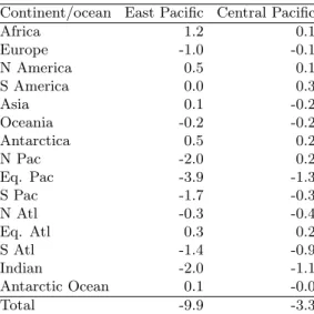
ENSO. The anomaly maps are shown on Figure 4. The total 187
friction torque is at the level of 10 Hadleys for EP ENSO, 188
and about a third for CP ENSO, with maximum effect over 189
the Pacific and over the part of the Antarctic Ocean, North 190
of the Indian Ocean, as seen on Table 2. The stronger fric-191
tion in the case of EP ENSO is logical, considering that the 192
wind anomaly is stronger in the CP ENSO case. A stronger 193
friction torque is also necessary to break down the larger 194
AAM anomaly resulting from the larger mountain torque in 195
the EP ENSO case. 196
5. Conclusions
In this paper, we investigate the impact of the ENSO on 197
the Earth rotation, and show that the AAM signature of the 198
Eastern Pacific type of ENSO is more than twice as large 199
than that of the Central Pacific ENSO. We then explain this 200
difference using the torque approach, as it allows us to de-201
termine where and how the AM is exchanged between the 202
solid Earth and the atmosphere. As expected, we also find 203
stronger torques for the EP ENSO, for both the mountain 204
and the friction torque. The ratio of the dominant mountain 205
torque created by the Eastern Pacific events to that created 206
by the Central Pacific events varies between 1.5 and 3.0 207
with the ratio on the total mountain torque being 2.6. The 208
strongest contributing continents are Asia, North and South 209
America and Africa. For the frictional torque, this ratio is 210
3.0. Looking at the associated surface pressure anomaly, 211
we show that the pressure dipole for EP ENSO is posi-212
tioned so that there is a strong East-West pressure gradient 213
over the major mountain ranges: Himalayas, Andes, Rocky 214
Mountains, whereas the pressure dipole for CP ENSO is 215
not as efficiently positioned. The stronger mountain torque 216
explains the stronger AAM anomaly. The stronger wind as-217
sociated with the anomaly generate a stronger negative fric-218
tion torque at the Earth surface, which cancels the AAM 219
anomaly. 220
This case study demonstrates how the torque approach 221
provides additional insights, explaining the AAM changes. 222
In this case, it allows to provide an explanation as why the 223
two types of ENSO events do not have the same impact on 224
the Earth rotation. 225
Acknowledgments. We gratefully acknowledge discussions 226
with Tong Lee regarding the two ENSO type literatures. This
227
study was supported by the CNES through the TOSCA program,
228
and by the Institut Universitaire de France (OdV). The work of
229
JOD is a phase of research carried out at the Jet Propulsion
230
Laboratory, California Institute of Technology, sponsored by the
231
National Aeronautics and Space Administration (NASA). It is a
232
pleasure to thank the editor (Eric Calais) and two anonymous
233
reviewers for their help in improving the paper.
234
References
Ashok, K., and T. Yamagata (2009), Climate Change The El
235
Nino with a difference, Nature, 461 (7263), 481–484, doi:
236
10.1038/461481a.
237
Ashok, K., S. K. Behera, S. A. Rao, H. Weng, and T. Yamagata
238
(2007), El Nino Modoki and its possible teleconnection, J. of
239
Geophys. Res.-Ocean, 112 (C11), doi:10.1029/2006JC003798.
240
Barnes, R., R. Hide, A. White, and C. Wilson (1983),
Atmo-241
spheric angular momentum fluctuations, length-of-day changes
242
and polar motion, Proceedings of the Royal Society of London.
243
A. Mathematical and Physical Sciences, 387 (1792), 31–73.
244
Burden, R., and J. Faires (2010), Numerical Analysis, Cengage
245
Learning.
246
Chao, B. (1984), Interannual length-of-day variation with
rela-247
tion to the Southern Oscillation/El-Nino, Geophys. Res. Let.,
248
11 (5), 541–544, doi:10.1029/GL011i005p00541.
249
Chao, B. F. (1988), Correlation of Interannual Length-of-Day
250
Variation With El-Ni˜no/Southern Oscillation, 1972-1986, Jo.
251
of Geophys. Res., 93 (B7), 7709–7715.
252
Clarke, A. (2008), An Introduction to the Dynamics of El Nino
253
& the Southern Oscillation, Elsevier Science.
254
Davis, J. (1986), Statistics and Data Analysis in Geology, John
255
Wiley & Sons.
256
de Viron, O., and V. Dehant (2003), Tests on the validity of
at-257
mospheric torques on earth computed from atmospheric model
258
outputs, J. of Geophys. Res., 108 (B2), 2068.
259
de Viron, O., S. Marcus, and J. Dickey (2001), Atmospheric
260
torques during the winter of 1989: Impact of ENSO and NAO
261
positive phases, Geophys. Res. Lett, 28 (10), 1985–1988.
262
de Viron, O., J. O. Dickey, and S. L. Marcus (2002), Annual
at-263
mospheric torques: Processes and regional contributions,
Geo-264
phys. Res. Let., 29 (7), 44–1–44–3, doi:10.1029/2001GL013859.
265
de Viron, O., S. Marcus, and J. Dickey (2001), Atmospheric
266
torques during the winter of 1989: Impact of ENSO and NAO
267
positive phases, Geophys. Res. Let., 28 (10), 1985–1988.
268
Hide, R., and J. O. Dickey (1991), Earth’s variable rotation,
Sci-269
ence, 253, 629–637.
270
Huang, H., P. Sardeshmukh, and K. Weickmann (1999), The
271
balance of global angular momentum in a long-term
atmo-272
spheric data set, Journal of Geophysical Research:
Atmo-273
spheres, 104 (D2), 2031–2040, doi:10.1029/1998JD200068.
274
Kalnay, E., M. Kanamitsu, R. Kistler, W. Collins, D. Deaven,
275
L. Gandin, M. Iredell, S. Saha, G. White, J. Woollen,
276
Y. Zhu, M. Chelliah, W. Ebisuzaki, W. Higgins, J. Janowiak,
277
K. Mo, C. Ropelewski, J. Wang, A. Leetmaa, R. Reynolds,
278
R. Jenne, and D. Joseph (1996), The NCEP/NCAR 40-year
279
reanalysis project, Bull. Am. Met. Soc., 77 (3), 437–471, doi:
280
10.1175/1520-0477(1996)077.
281
Kao, H.-Y., and J.-Y. Yu (2009), Contrasting Eastern-Pacific and
282
Central-Pacific Types of ENSO, J. of Clim., 22 (3), 615–632,
283
doi:10.1175/2008JCLI2309.1.
284
Kim, H.-M., P. J. Webster, and J. A. Curry (2009), Impact
285
of Shifting Patterns of Pacific Ocean Warming on North
286
Atlantic Tropical Cyclones, Science, 325 (5936), 77–80, doi:
287
10.1126/science.1174062.
288
Kug, J.-S., F.-F. Jin, and S.-I. An (2009), Two Types of El Nino
289
Events: Cold Tongue El Nino and Warm Pool El Nino, J.
290
Clim., 22 (6), 1499–1515, doi:10.1175/2008JCLI2624.1.
291
Larkin, N., and D. Harrison (2005), Global seasonal temperature
292
and precipitation anomalies during El Nino autumn and
win-293
ter, Geophys. Res. Let., 32 (16), doi:10.1029/2005GL022860.
294
Latif, M., R. Kleeman, and C. Eckert (1997), Greenhouse
warm-295
ing, decadal variability, or El Nino? An attempt to
under-296
stand the anomalous 1990s, J. of Clim., 10 (9), 2221–2239,
297
doi:10.1175/1520-0442(1997) 010<2221:GWDVOE>2.0.CO;2.
298
Lott, F., O. De Viron, P. Viterbo, and F. Vial (2008), Axial
atmo-299
spheric angular momentum budget at diurnal and subdiurnal
300
periodicities, J. Atm. Sc., 65 (1), 156–171.
301
Marcus, S. L., O. de Viron, and J. O. Dickey (2010), Interannual
302
atmospheric torque and El Ni˜no–Southern Oscillation: Where
303
is the polar motion signal?, J. of Geophys. Res., 115 (B12),
304
B12,409.
305
Marcus, S. L., O. de Viron, and J. O. Dickey (2011), Abrupt
306
atmospheric torque changes and their role in the 1976-1977
307
climate regime shift, J. of Geophys. Res.-Atmosphere, 116,
308
doi:10.1029/2010JD015032.
309
Ponte, R. M., and R. D. Rosen (1999), Torques responsible for
310
evolution of atmospheric angular momentum during the
1982-311
83 El Ni˜no, J. of the Atm. Sci., 56 (19), 3457–3462.
312
Ren, H.-L., and F.-F. Jin (2011), Nino indices for two types of
313
ENSO, Geophys. Res. Let., 38, doi:10.1029/2010GL046031.
314
Weng, H., S. K. Behera, and T. Yamagata (2009), Anomalous
315
winter climate conditions in the Pacific rim during recent El
316
Ni˜no Modoki and El Ni˜no events, Clim. Dyn., 32 (5), 663–674,
317
doi:10.1007/s00382-008-0394-6.
318
Widger, W. K. (1949), A study of the flow of angular momentum
319
in the atmosphere, J. Meteor, 6, 292299.
X - 4 DE VIRON ET AL.: TWO EL-NINO AND LOD VARIATIONS −1.5 −1 −0.5 0 0.5 1 1.5 −0.2 −0.1 0 0.1 0.2 AAM anomaly (10 2 5 kg m 2/s) LOD anomaly (10 − 3 s) N EP NCP
{
{
t EP + t CP + t EP 0 t CP 0 t EP − t CP − σFigure 1. Whisker diagram of the AAM during times
where indices (NEP on the left, NCP on the right) are
1-σ above average, below average, or at the neutral state.
East Pacific
Central Pacific
−3.00 −2.25 −1.50 −0.75 0.00 0.75 1.50 2.25 3.00
Figure 2. Difference in surface pressure anomaly
be-tween positive and negative phase of NEP and NCP, as
defined in equation(11).
Wolf, W., and R. Smith (1987), Length-of-day changes and
moun-321
tain torque during el ni˜no, J. of the Atm. Sci., 44, 3656–3660.
322
Yu, J. Y., and S. T. Kim (2010), Three evolution patterns
323
of Central-Pacific El Nino, Geophys. Res. Let., 37, doi:
324
10.1029/2010GL042810.
Ea
ste
rn
Pa
cifi
c a
no
ma
ly
Andes
Rocky Mountains
Hymalayas
Ce
ntr
al
Pa
cif
ic
an
om
aly
−3.0 −2.4 −1.8 −1.2 −0.6 0.0 0.6 1.2 1.8 2.4
Figure 3. Difference in surface pressure anomaly
be-tween positive and negative phase of NEP and NCP, as
defined in equation(11), focused on the major mountain ranges (Andes on the left, Rocky Mountains on the cen-ter, and Himalayas on the right). The top panel is for EP anomaly and the bottom one for the CP anomaly.
East Pacific
Central Pacific
−1.2 −0.6 0.0 0.6 1.2
Figure 4. Difference in zonal friction drag anomaly
be-tween positive and negative phase of NEP and NCP, as
defined in equation(11). The top panels is for the EP anomaly and the bottom one for the CP anomaly.
X - 6 DE VIRON ET AL.: TWO EL-NINO AND LOD VARIATIONS
Table 1. Mountain torque (in Hadley, i.e. 1018N m),
com-puted from CEP and CCP of the surface pressure, computed as explained by equation (11).
Continent East Pacific Central Pacific
Africa 1.2 0.8 Europe -0.4 0.1 N America 1.7 1.0 S America 1.1 0.0 Asia 1.7 0.2 Oceania 0.2 -0.1 Antarctica -0.1 0.1 Total 5.4 2.1
Table 2. Friction torque (in Hadley, i.e. 1018 N m),
com-puted from CEP and CCP of the friction drag, computed as explained by equation (11). The separation map for the ocean/continent can be found in Figure 3 of Marcus et al. [2011].
Continent/ocean East Pacific Central Pacific
Africa 1.2 0.1 Europe -1.0 -0.1 N America 0.5 0.1 S America 0.0 0.3 Asia 0.1 -0.2 Oceania -0.2 -0.2 Antarctica 0.5 0.2 N Pac -2.0 0.2 Eq. Pac -3.9 -1.3 S Pac -1.7 -0.3 N Atl -0.3 -0.4 Eq. Atl 0.3 0.2 S Atl -1.4 -0.9 Indian -2.0 -1.1 Antarctic Ocean 0.1 -0.0 Total -9.9 -3.3