HAL Id: hal-00299441
https://hal.archives-ouvertes.fr/hal-00299441
Submitted on 1 Aug 2007
HAL is a multi-disciplinary open access
archive for the deposit and dissemination of
sci-entific research documents, whether they are
pub-lished or not. The documents may come from
teaching and research institutions in France or
abroad, or from public or private research centers.
L’archive ouverte pluridisciplinaire HAL, est
destinée au dépôt et à la diffusion de documents
scientifiques de niveau recherche, publiés ou non,
émanant des établissements d’enseignement et de
recherche français ou étrangers, des laboratoires
publics ou privés.
The development of the INGV tectonomagnetic network
in the frame of the MEM Project
F. Masci, P. Palangio, M. Di Persio, C. Di Lorenzo
To cite this version:
F. Masci, P. Palangio, M. Di Persio, C. Di Lorenzo. The development of the INGV tectonomagnetic
network in the frame of the MEM Project. Natural Hazards and Earth System Science, Copernicus
Publications on behalf of the European Geosciences Union, 2007, 7 (4), pp.473-478. �hal-00299441�
www.nat-hazards-earth-syst-sci.net/7/473/2007/ © Author(s) 2007. This work is licensed under a Creative Commons License.
and Earth
System Sciences
The development of the INGV tectonomagnetic network in the
frame of the MEM Project
F. Masci, P. Palangio, M. Di Persio, and C. Di Lorenzo
Istituto Nazionale di Geofisica e Vulcanologia, Italy
Received: 28 June 2007 – Revised: 12 July 2007 – Accepted: 12 July 2007 – Published: 1 August 2007
Abstract. In the middle of 1989, the INGV (Italian
Isti-tuto Nazionale di Geofisica e Vulcanologia) installed in Cen-tral Italy a network of magnetic stations in order to inves-tigate possible relationship of the local magnetic field with earthquakes occurrences. Actually the network consists of four stations, where the total magnetic field intensity data are being collected using proton precession magnetometers. Here we are report on the actual state and the future develop-ments of the network. In the frame of the MEM (Magnetic and Electric fields Monitoring) Project, new stations will be added to the network by the end of 2007. The results of the test campaigns carried out in the sites chosen to widen the network are also discussed. Moreover, the 2006 complete data set of the network is also reported. Concerning the data analysis, a new approach is also discussed that takes into ac-count the inductive effects on the local geomagnetic field by means of the inter-station transfer functions time variations analysis.
1 Introduction
Stress changes in the Earth’s crust associated with the seis-mic and volcanic activity can be linked to local magnetic anomalies (Stacey, 1964; Hayakawa and Fujinawa, 1994; Molchanov et al., 1995; Johnston, 1997; Johnston and Parrot, 1998). The observation of these anomalies is quite difficult because their amplitude depends principally on the intensity of the seismic events, on the involved physical mechanisms and on the distance between the earthquake hypocenter and the observation point (Hayakawa et al., 2007). Moreover, coseismic field changes are larger than preseismic and post-seismic changes because the observed copost-seismic effects are due to the release of the accumulated crustal stress during Correspondence to: F. Masci
the entire earthquake duration, whereas the preseismic sig-nals are due to a small fraction of the accumulated energy release (Mueller and Johnston, 1998). For this the reason the precursory signals linked to earthquakes occurrence are difficult to detect. In any case, the value of these anomalies, approximately a few nT, is very small with respect to the total field value. From the seismic point of view, Italy is an area with several active faults (see Fig. 1) and, in the past, has been characterized by a lot of wasteful earthquakes. In Cen-tral Italy several studies concerning the correlation between anomalous electromagnetic signals and the tectonic activ-ity can be found in the literature (De Lauretis et al., 1995; Biagi et al., 2002). Bella et al. (1998) described anoma-lous acoustic, electric and magnetic signals related to the M=3.9 Gran Sasso earthquake occurred on 25 August 1992. The INGV tectonomagnetic network was installed in Central Italy since the middle of 1989. The network is spread out in
an area extending approximately in the latitude range [41.6◦–
42.8◦]N and longitude range [13.0◦–14.3◦]E. Until now, no
evident correlation between tectonic activity in Central Italy and changes in the local magnetic field has been observed. In the last three years some inexplicable events in one sta-tion of the network have occurred (Masci et al., 2006), but no evident relationship with the local earthquakes has been found.
2 Working and planned stations
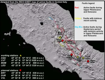
The INGV tectonomagnetic network is part of the INGV L’Aquila Geomagnetic Observatory and at the present time, total magnetic field intensity data are collected in four sta-tions using proton precession magnetometers. The network stations are: L’Aquila (AQU), Monte di Mezzo (MDM), Civitella Alfedena (CVT) and Leonessa (LEO). In Fig. 1 the location in Central Italy of the four stations are reported. The sampling rate of each station is set to 15 min except for the
474 F. Masci et al.: The development of the INGV tectonomagnetic network in the frame of the MEM project
Faults legend
Red: Active faults during
Upper Pleistocene and Holocene
Yellow: Faults with dubious recent activity
Sky-Blu: Active faults during Quaternary period with dubious activity in Upper Pleistocene and Holocene MDM CVT AQU LEO DUR VVL working stations AQU 42° 23' N 13° 19' E 682 m a.s.l. CVT 41° 47' N 13° 54' E 1020 m a.s.l. MDM 41° 46' N 14° 13' E 980 m a.s.l. LEO 42° 33' N 13° 04' E 1320 m a.s.l. planned stations BRT 42° 30' N 13° 16' E 930 m a.s.l. DUR 41° 39' N 14° 27' E 910 m a.s.l. VVL 41° 52' N 13° 37' E 960 m a.s.l.
Adapted from the INGV-GNDT map of active faults in Central Italy
BRT
Figure 1. The locations of the INGV tectonomagnetic network stations in Central Italy are Fig. 1. The locations of the INGV tectonomagnetic network stations
in Central Italy are shown. The faults distribution in the Central Apennines is also reported.
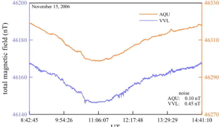
AQU Observatory in which the sampling rates are 1 min and 1 s. In the frame of the MEM Project (Interreg IIIA Adri-atic Cross Border Programme) has been decided to upgrade the network. The MEM Project has been activated in the INGV Observatory of L’Aquila since 2004 (Palangio et al., 2007). The leader partner of the project is the Italian Abruzzo Region. The other partners are the INGV Observatory of L’Aquila, the Regional Environmental Agency of Molise Re-gion (ARPA-Molise), Italy, the University of Ferrara, Italy, the University of Tirana, Albania and the Geomagnetic In-stitute of Grocka, Beograd, Serbia. During the 2007 new stations will be added to the network with the aim to fill the network’s gaps and to extend the research area. Moreover, the instrumentation of each station will be updated in order to widen the frequency band till 1 Hz and to get vectorial mag-netic data. Each station of the network will be supplied with an Overhauser magnetometer and a 3-axial magnetometer. At the middle of the 2006, three potential sites were chosen taking into account in the beginning the logistics problems and the distance of the sites from the human activities. Fig-ure 1 illustrates the locations of these sites: Barete (BRT), Duronia (DUR) and Villavallelonga (VVL). In a second step some test campaigns have been planned to check the elec-tromagnetic background noise level of these sites. The AQU station was chosen as a reference station for the test cam-paigns. The background noise level of the magnetic field recorded in the AQU station is about 0.1 nT peak-to-peak. In Figs. 3 and 4, as examples of good and bad site for mag-netic measurements, the results of the test campaigns carried out in Duronia and Villavallelonga, respectively on 9 and 15 November 2006, are shown. The test campaigns have been performed using an Overhauser magnetometer and the col-lected data sets have been compared with the AQU total
mag-46000 46100 46200 46300 46400 46500 da il y m ea n of t h e to ta l m ag n et ic fi el d (n T ) AQU MDM CVT 180 182 184 186 188 190 230 232 234 236 238 240 d ai ly m ea n of t h e t o ta l m ag n et ic f ie ld d if fe re n ce s ( n T ) 0 30 60 90 120 150 180 210 240 270 300 330 360 2006 Julian Day 45 47 49 51 53 55 MDM - CVT AQU - CVT AQU - MDM
Figure 2. Top: 2006 data set reported as daily means of the total magnetic field recorded in Fig. 2. Top: 2006 data set reported as daily means of the total
mag-netic field recorded in each network station. Bottom: 2006 daily means of the total magnetic field differences for the couple of sta-tions AQU-CVT, AQU-MDM, MDM-CVT. The colour of each plot is the same of the corresponding vertical axis.
netic field measured in the same period of time. Looking at Fig. 3, both the signals show the same principal structures showing only small differences due to the local variations of the magnetic field. Moreover, it is evident that the noise of the DUR signal (≈0.15 nT peak-to-peak) is comparable with the noise of the AQU signal. We have obtained the same re-sults in the test campaign carried out in the BRT site. So, these two sites will be enclosed in the network. Looking at Fig. 4 it is obvious that the VVL signal is unfortunately nois-ier than the AQU signal; the background noise level is about 0.5 nT peak-to-peak. The explanation of the VVL noise can be found in the electrified railway some kilometers far away from the site (Palangio et al., 1991). So this site has been rejected and we are searching for a new site to fill the gap between AQU and CVT stations.
3 The 2006 data set
In the top panel of Fig. 2 is reported the 2006 data set of the network as daily means of the total magnetic field. Each sta-tion data set is differentiated with respect to the data set of the other stations in order to detect any local field anoma-lies. The differentiation procedure removes the contributions from other sources, external (i.e. electric currents in the iono-sphere and magnetoiono-sphere) and internal to the Earth (i.e. sec-ular trend of the geomagnetic field). The only one remaining
11:24:40 12:06:32 12:48:25 13:30:17 14:12:10 UT 46210 46220 46230 46240 46250 to ta l m ag n e ti c fi el d ( n T ) 46310 46320 46330 46340 46350 DUR AQU November 9, 2006 noise AQU: 0.10 nT DUR: 0.15 nT
Figure 3. Duronia test campaign data set compared with L’Aquila measurements. The Fig. 3. Duronia test campaign data set compared with L’Aquila
measurements. The acquisition time step is 5s. The colour of each plot is the same of the corresponding vertical axis. Note that the noise of the DUR data set is comparable with the noise of the AQU data set. In the MDM signal the evident noise at 13:05 UT is due to a mushroom seeker walking near the sensor.
is due to the local variation in crustal magnetization and to the tectonic activity as well. A daily mean of the differenti-ated data is calculdifferenti-ated to remove the diurnal variation. The LEO station data set is not reported in the figure because of the large number of gaps in the data due to technical prob-lem which affect the continuity of the measurements. The bottom panel of Fig. 2 shows the differences among the sta-tions of AQU, CVT and MDM as daily means. During the 2006 no significant seismic activity has been registered in Central Italy. The maximum magnitude of the local earth-quakes registered during this period is about M=3.5 (INGV Seismic Bulletin, 2006), so no significant anomalies in the lo-cal geomagnetic field are expected. In any case in Fig. 2 the differentiated data indicate some events that can mislead us. Looking at the figure, the presence of two jumps is obvious between two levels with a difference of 2 nT and 4 nT respec-tively, in the days JD=13 and JD=136. These events are due to the MDM total geomagnetic field as they are present in the differences AQU-MDM and MDM-CVT and are not evident in the differences AQU-CVT. In the previous years similar events are shown for the MDM station. We can exclude in-strumental problems as after the first event of 2004 we have changed the MDM instrumentation with a new magnetome-ter, but about a year later we have recorded another event with the new instrumentation (Masci et al., 2006). Figure 2 shows probably a similar event happened unfortunately dur-ing the gap JD=160–277 in the MDM data set as can be seen by the different levels of the MDM-CVT and AQU-MDM differentiated data. Anyway, we want to point out that there are no relations between these jumps and the seismic activ-ity. At this time, we have no reasonable explanation for these events. To better investigate the kind of these jumps, in the MDM station, from the end of 2006, a second magnetome-ter that is working simultaneously with the existing station
8:42:45 9:54:26 11:06:07 12:17:48 13:29:29 14:41:10 UT 46140 46160 46180 46200 to ta l m a g n e ti c f ie ld ( n T ) 46270 46290 46310 46330 AQU VVL noise AQU: 0.10 nT VVL: 0.45 nT November 15, 2006
Figure 4. Villavallelonga test campaign data set compared with L’Aquila measurements. The
Fig. 4. Villavallelonga test campaign data set compared with
L’Aquila measurements. The acquisition time step is 5 s. The colour of each plot is the same of the corresponding vertical axis. Note the remarkable noise of the VVL signal probably due to the electrified railway some kilometers faraway from the site. This site has been rejected.
instrumentation was installed. The instrument is an Over-hauser magnetometer with an acquisition time step set to 5 s.
4 The inter-stations transfer functions analysis
A new approach in the data analysis, which takes into ac-count the inductive effects, has been tested by means of the temporal variation of inter-station transfer functions. This kind of analysis takes into account the electric currents in-duced in the Earth’s electrically conducting layer that in turn produce a magnetic field on the Earth’s surface. The electric conductivity of the rocks is an important physical measurable property of the Earth’s crust. The conductivity time varia-tion can be monitored by the study of the magnetic trans-fer functions temporal variation, and therefore by the associ-ated magnetic induction vectors variation. So, the monitor-ing of the transfer functions is an available method to study the crustal conductivity changes in the vicinity of the mea-surement site. Usually, this kind of analysis is focused on the monitoring of the transfer functions evaluated by the varia-tion of the geomagnetic field components measured in the same place (station transfer functions). The single-station transfer functions analysis provides information on the electrical conductivity profile under the area of the mea-surement site. On the contrary, the inter-station transfer func-tions (ISTF) analysis provides information on the difference of the Earth’s crust electrical conductivity structure between two sites. Some examples concerning the changes of the magnetic transfer functions related to the seismic activity are reported in the literature (see for example Yanagihara and Nagano, 1976; Harada et al., 2004). Using the ISTF tech-nique, Chen et al. (2006) have reported two significant trans-fer functions anomalies 40 and 20 months before two high seismic events. Moreover, they have shown that the transfer
476 F. Masci et al.: The development of the INGV tectonomagnetic network in the frame of the MEM project
1E-004 1E-003 1E-002 1E-001
ω (Hz) 0.0 0.2 0.4 0.6 0.8 1.0 1.2 1.4 IS T FM D M -A Q U Jan 2007 Feb 2007
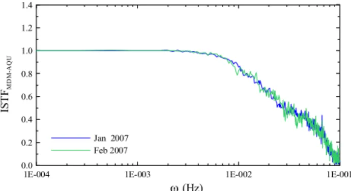
Fig. 5. Inter station transfer functions (ISTF) estimated between
AQU and MDM stations for the months January and February 2007 using the total magnetic field data.
functions change is a local effect rather than a large scale effect and that only long-term precursory effects can be de-tected. Actually, waiting for the upgrade of the our stations with 3-axial magnetometers, for this kind of analysis we use the total field data of the new Overhauser magnetometer in-stalled in MDM and the vectorial data set of the AQU ob-servatory. The data time resolution is 5 s. First of all we are testing if the variations of the inter-station transfer func-tions, estimated from the total magnetic field data measured in two stations of the network can be related also to the rel-ative changes of the crustal conductivity. In that case, the
transfer function Txy(ω), can be defined in the frequency
do-main as the ratio of the cross spectrum Pxy(ω)and the power
spectrum Pxx(ω):
Txy(ω) =
Pxy(ω)
Pxx(ω)
(1) In Eq. (1) x(t ) and y(t ) are the total magnetic field measured in two stations of the network as a function of time t, and
ω represents the frequency. However, these transfer
func-tions are not completely independent of the horizontal field components because they depend both on the magnetic incli-nation and on the variations of the magnetic decliincli-nation of the measurement sites. As example, in Fig. 5 are shown the monthly mean transfer functions for the couple of stations AQU and MDM evaluated for January and February 2007. Note that the two transfer functions have a similar behaviour. In the frequency band [0–0.005]Hz the value of the transfer functions is about 1, so the spectral content of the signals col-lected in the two sites is the same. Above 0.005 Hz the differ-ences among the two sites are evident. With the assumption that the variations of the magnetic field horizontal compo-nents are the same in the two sites, this difference can be linked with the inductive effects due to the different spectral response of the measurement sites. This different spectral re-sponse can be directly connected with the differences of the underground electric conductivity structure in the two sites. Looking at Fig. 5 it is obvious that the two transfer
func-tions look like a low pass filter transfer function with a cut-off frequency around 0.015Hz. This frequency corresponds to an estimated skin-depth which involves the whole Earth’s crust in the observed area. Therefore, in our case the role of the inductive effects should be significant for frequencies higher than the cut-off frequency. A second approach has been tested according to Hitchman et al. (2000). In that case, the inter-station transfer functions have been evaluated by the total magnetic field measured in a station and the variation of the horizontal field components recorded in a reference site. They applied this technique to aeromagnetic base station data and to data set collected at the sea surface by offshore floating magnetometer. If Z, H and D are respectively the variations of the vertical component and the north and east horizontal components of the geomagnetic field, we can assume, in the frequency domain, the relation
Z(ω) = A(ω)H (ω) + B(ω)D(ω) (2)
where A(ω) and B(ω) are the magnetic transfer functions and ω is the frequency. A(ω) and B(ω) are generally com-plex functions. They are time invariant functions if the elec-tric resistivity of the ground does not change; that is, when no large crustal changes due to geodynamical processes are in progress. If we know the total field F but not the vertical
component Z, we can define AF(ω)and BF(ω)as the
trans-fer functions related to the total field (Lilley et al., 1984) and we can write
F (ω) = AF(ω)H (ω) + BF(ω)D(ω) (3) In the frequency domain, F (ω) can be written as
F(ω)=H(ω)cos I + Z(ω)sinI (4)
where I is the local inclination. The value of the inclination
used in the calculation is I = 57,8◦. Comparing Eq. (2) and
Eq. (4) we obtain
F (ω) = H (ω)[A(ω) sin I + cosI ] + D(ω)B(ω)sinI (5) So, from Eq. (3) and Eq. (5), we obtain
AF(ω) = A(ω)sin I + cos I (6)
BF(ω) = B(ω)sin I
Starting from A(ω) and B(ω) obtained from Eq. (6), we can define a pair of induction vectors, each corresponding to the real and imaginary components, whose magnitudes are:
|T (ω)|r = p Ar(ω)2+Br(ω)2 (7) |T (ω)|i = p Ai(ω)2+Bi(ω)2 whereas the corresponding phases are
2(ω)r =tan−1[Br(ω)/Ar(ω)] (8)
2(ω)i =tan−1[Bi(ω)/Ai(ω)]
-180 -135 -90 -45 0 45 90 135 180 θ (° ) 0 0.01 0.02 0.03 0.04 0.05 0.06 0.07 0.08 0.09 0.1 ω(Hz) 0 0.5 1 1.5 |T | real imag
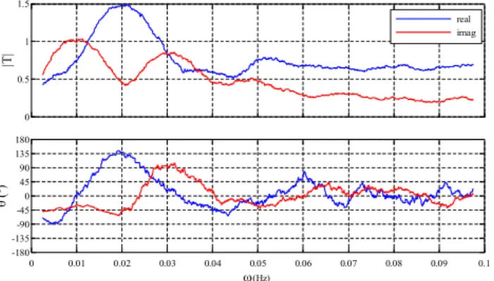
Fig. 6. Magnitude and phase of the induction vectors estimated for
20 January 2007 using the MDM total magnetic field and the AQU magnetic horizontal components.
In Eq. (7) and Eq. (8) the subscripts r and i refer to the real and imaginary components respectively. For this kind of analysis we use the MDM total magnetic field and the AQU horizontal field components. Figure 6 reports an example of the typical behaviour of the real and the imaginary induc-tion vectors as a funcinduc-tion of the frequency. The reported induction vectors refer to 20 January 2007. The imaginary vector can be linked with the resistive component of the sub-soil impedance, whereas the real vector is related to the re-active component which carries the current induced by the magnetic horizontal field variations. In Fig. 7 is reported the induction vectors time variation for the period from the mid-dle of December 2006 to the midmid-dle of February 2007 in the frequency band [0.05–0.1]Hz. This frequency interval can be related to the crustal depth within to the first 25 km. The induction vectors show the normal behaviour when no large crustal changes due to geodynamical processes are present. Anyway no significant local tectonic activity has been regis-tered in this period, so no significant anomalies in the local geomagnetic field is expected. In any case, the analysis of the data that will be collected in the future years in the INGV tectonomagnetic network will be necessary to check the va-lidity of the two reported methods.
5 Conclusions
We have reported the whole data set of the INGV tectono-magnetic network for the year 2006 both as daily means of the total magnetic field and as differences between each net-work data set. No correlation with the local seismic activity has been so far found. Anyway no significant seismic activ-ity has been registered in Central Italy in this period, so no significant anomalies in the local magnetic field is expected. Some misleading events are pointed out in one station of the network. The network upgrade in the frame of the MEM project is also discussed. The results of the test campaigns carried out in the sites planned as new stations of the network
-180 -135 -90 -45 0 45 90 135 180 θ (° ) 355 360 365 5 10 15 20 25 30 35 40 45 2006 2007 JD 0 0.5 1 1.5 |T | real imag Δω =[0.05-0.10] Hz
Figure 7. Induction vectors magnitudes and phases time variation for the period December Fig. 7. Induction vectors magnitudes and phases time variation for
the period December 2006–February 2007 in the frequency band [0.05–0.10]Hz.
are reported showing that one of these sites is not suitable for the installation of a tectonomagnetic station. A new ap-proach in the usual data analysis has been tested by means of the inter-station transfer functions evaluation. Two methods are tested using, in the first case, the total magnetic field data set of MDM and AQU stations and in the second the MDM total magnetic field combined with the AQU magnetic hori-zontal components. Future analysis of the data collected in the network stations will be necessary to check the validity of the two methods.
Acknowledgements. The authors are indebted to the L’Aquila
Observatory technical-administrative staff for the essential support in the research activity. This work was supported by the MEM Project (Interreg IIIA Adriatic Cross Border Programme).
Edited by: M. Contadakis
Reviewed by: O. Molchanov and another anonymous referee
References
Bella, F., Biagi, P. F., Caputo, M., Della Monica, G., Ermini, A., Plastino W., and Sgrigna, V.: Anomalies in different parameters related to the M=3.9 Gran Sasso earthquake (1992), Phys. Chem. Earth, 23, 9, 959–963, 1998.
Biagi, P. F., Ermini, A., Piccolo, R., Loiacono, D., and Kings-ley, S. P.: Electromagnetic signals related to micromovements of limestone blocks: A test in kart caves of Central Italy, Seismo Electromagnetics Lithosphere-Atmosphere-Ionosphere Coupling, 81–86, Eds M. Hayakawa and O. A. Molchanov, Ter-rapub, Tokyo, 2002.
Chen, K. J., Chiu, B., and Lin, C.: A search for a correlation between time change in transfer functions and seismic energy release in northern Taiwan, Earth Planets Space, 58, 981–991, 2006.
De Lauretis, M., De Luca, G., Scarpa, R., and Villante, U.: ULF ge-omagnetic field measurements during local seismic events, Atti XIV◦Convegno GNGTS, Roma, 23–25 October, 1995.
478 F. Masci et al.: The development of the INGV tectonomagnetic network in the frame of the MEM project
Harada, M., Hattori, K., and Isezaki, N.: Transfer function approach to signal discrimination of ULF geomagnetic data, Phys. Chem. of Earth, 29, 409–417, 2004.
Hayakawa, M. and Fujinawa, Y. (Editors): Electromagnetic Phe-nomena Related to Earthquake Prediction, Terra Sci. Pub. Comp., Tokyo, pp. 677, 1994.
Hayakawa, M., Hattori K., and Ohta, K.: Monitoring of ULF(ultra-low-frequency) geomagnetic variations associated with Earth-quakes, Sensors, 7, 1108–1122, 2007.
Hitchman, A. P., Lilley, F. E. M., and Milligan, P. R.: Induction ar-rows from offshore floating magnetometers using land reference data, Geophys. J. Int., 140, 442–452, 2000.
INGV (Istituto Nazionale di Geofisica e Vulcanologia): Seismic Bullettin, Roma, 2006.
Johnston, M. J. S.: Review of electrical and magnetic fields ac-companying seismic and volcanic activity, Surv. Geophys., 18, 441–475, 1997.
Johnston, M. J. S. and Parrot, M.: Electromagnetic effects of earth-quakes and volcanoes, Phys. Earth Planet. In., Special Volume, 105, 109–295, 1998.
Lilley, F. E. M., Sloane, M. N., and Fergusson, I. J.: An applica-tion of the total-field magnetic fluctuaapplica-tion data to geomagnetic induction studies, J. Geomagn. Geolectr., 36, 161–172, 1984. Masci, F., Palangio, P., and Meloni, A.: INGV tectonomagnetic
network: 2004–2005 preliminary dataset analysis, Nat. Hazards Earth Syst., 6, 773–777, 2006.
Molchanov, O. A., Hayakawa, M., and Rafalsky, V. A.: Penetra-tion characteristics of electromagnetic emissions from an under-ground seismic source into the atmosphere, ionosphere and mag-netosphere, J. Geophys. Res., 100, A2, 1691–1712, 1995. Mueller, R. J. and Johnston, M. J. S.: Review of magnetic field
monitoring near active faults and volcanic calderas in California: 1974–1995, Phys. Earth Planet. In., Special Volume, 105, 131– 144, 1998.
Palangio, P., Marchetti, M., and Di Diego, L.: Rumore elettro-magnetico prodotto dalle ferrovie elettrificate. Effetti sulle mis-ure magnetotelluriche e geomagnetiche, Atti del X Convegno GNGTS, 126–139, 1991.
Palangio, P., Di Lorenzo, C., Di Persio, M., Masci, F., Mihajlovic, S., Santarelli, L., and Meloni, A.: Electromagnetic monitoring of the Earth’s interior in the frame of MEM project, submitted to Ann. Geoph-Italy, 2007.
Stacey, F. D.: The seismomagnetic effect, Pure Appl. Geophys., 58, 5–22, 1964.
Yanagihara, K. and Nagano, T.: Time change of transfer function in the central Japan anomaly of conductivity with special reference to earthquakes occurrences, J. Geomagn. Geoelectr., 28, 157– 163, 1976.