The role of soil states in medium-range weather predictability

HAL Id: hal-00302049

https://hal.archives-ouvertes.fr/hal-00302049

Submitted on 1 Jan 2001

HAL is a multi-disciplinary open access

archive for the deposit and dissemination of

sci-entific research documents, whether they are

pub-lished or not. The documents may come from

teaching and research institutions in France or

abroad, or from public or private research centers.

L’archive ouverte pluridisciplinaire HAL, est

destinée au dépôt et à la diffusion de documents

scientifiques de niveau recherche, publiés ou non,

émanant des établissements d’enseignement et de

recherche français ou étrangers, des laboratoires

publics ou privés.

predictability

S. Fukutome, C. Prim, C. Schär

To cite this version:

S. Fukutome, C. Prim, C. Schär. The role of soil states in medium-range weather predictability.

Nonlinear Processes in Geophysics, European Geosciences Union (EGU), 2001, 8 (6), pp.373-386.

�hal-00302049�

Nonlinear Processes

in Geophysics

c

European Geophysical Society 2001

The role of soil states in medium-range weather predictability

S. Fukutome, C. Prim, and C. Sch¨ar

Atmospheric and Climate Science ETH, Winterthurerstr. 190, CH-8057 Z¨urich, Switzerland Received: 28 September 2000 – Revised: 2 April 2000 – Accepted: 17 April 2001

Abstract. Current day operational ensemble weather

pre-diction systems generally rely upon perturbed atmospheric initial states, thereby neglecting the eventual effect on the at-mospheric evolution that uncertainties in initial soil temper-ature and moisture fields could bring about during the sum-mer months. The purpose of this study is to examine the role of the soil states in medium-range weather predictability. A limited area weather prediction model is used with the atmos-phere/land-surface system in coupled or uncoupled mode. It covers Europe and part of the north Atlantic, and is driven by prescribed sea-surface temperatures over the sea, and by atmospheric reanalyses at its lateral boundaries.

A series of 3 member ensembles of summer simulations are used to assess the predictability of a reference simula-tion assumed to be perfect. In a first step, two ensembles are simulated: the first with the atmosphere coupled to the land-surface model, the second in the uncoupled mode with perfect soil conditions prescribed every 6 hours. Subsequent experiments are combinations thereof, in which the uncou-pled and couuncou-pled modes alternate in the course of a simula-tion.

The results show that there are “stable” and “unstable” pe-riods in the weather evolution under consideration. During the stable periods, the predictability (measured in terms of ensemble spread at 500 hPa) of the coupled and uncoupled dynamical systems is almost identical; prescribing the per-fect soil conditions has a negligible impact upon the atmo-spheric predictability. In contrast, the predictability during an unstable phase is found to be remarkably improved in the uncoupled ensembles. This effect results from guiding the at-mospheric phase-space trajectory along its perfect evolution. It persists even when switching back from the uncoupled to the coupled mode prior to the onset of the unstable phase, a result that underlines the importance of soil moisture and

Correspondence to: S. Fukutome

(fukutome@geo.umnw.ethz.ch)

temperature in data assimilation systems.

1 Introduction

Weather predictability for time scales from a few days to sev-eral months is often addressed by means of an ensemble pre-diction system (EPS). Rather than relying upon one deter-ministic simulation, a set of simulations with slightly differ-ing initial conditions is performed, and subsequently, statisti-cally analyzed with respect to the coherence between differ-ent members of the ensemble (Molteni et al., 1996). Deter-mining the associated initial perturbations is a delicate task, and is meant to reflect both uncertainties in the initial condi-tions and in the model formulation. Optimal perturbacondi-tions (in the sense discussed in the literature) may be obtained from singular vector methodologies, and span a particularly sensi-tive subspace in phase-space in the vicinity of the objecsensi-tive analysis (Buizza and Palmer, 1995). In currently operational procedures of this kind, the ensemble members are generated by perturbing the atmosphere without altering the soil condi-tions, thereby assuming that the latter plays no significant role in the subsequent atmospheric evolution.

This approach is meaningful for extratropical winter me-dium-range forecasts, in which the essential preoccupation is to reproduce the storm track accurately. In the extratropical summer and in the tropics, however, the atmospheric evolu-tion is less strongly dominated by the large-scale circulaevolu-tion, and other more local processes may come to play an impor-tant role. In recent years, much attention has been devoted to soil-atmosphere feedback processes. For the extratrop-ics, for instance, recent research has addressed such topics as: the role of initial soil moisture conditions in determin-istic medium-range forecasts (e.g. Viterbo and Betts, 1999; Beljaars et al., 1996); the role of soil-moisture storage and vegetation cover for global and regional climate simulations (e.g. Shukla and Mintz, 1982; Weatherald et al., 1995; Giorgi et al., 1996; Christensen, 1998; Heck et al., 2001); the

im-portance of land-surfaces for seasonal prediction (e.g. Pielke et al., 1999; Koster et al., 2000); and the feedback processes between soil moisture, convection and precipitation (Findell and Eltahir, 1997; Eltahir, 1998; Sch¨ar et al., 1999).

Thus, initialization of soil conditions turns out to be a cru-cial task. In order to counter this need, recent data assimila-tion studies have proposed to derive the soil moisture from the evolution of near-surface atmospheric parameters, using a method based either on optimal interpolation, or on vari-ational analysis (Mahfouf, 1991). The first has come to be called soil-moisture nudging (Hu et al., 1999) and was imple-mented in a somewhat simpler form in the European Center for Medium-range Weather Forecast (ECMWF) model. The second has been examined by Rhodin et al. (1999). Van den Hurk et al. (1997) also attempt to assimilate initial soil mois-ture fields from satellite imagery. The common feamois-ture of these methods is to update or re-initialize the soil moisture at regular intervals. Since it is generally assumed, however, that the effect of the soil moisture will not reach beyond the few lowest layers of the atmosphere, little work has been done to investigate the effect of the continuous updating on the evolution of the dynamical variables at higher levels. Never-theless, the study by Betts et al. (1996) seems to indicate that the nudging reduces the forecast error even at 200 hPa.

The purpose of the present study is to investigate how, if at all, the soil affects the predictability of the coupled atmo-sphere/soil system, with particular regard to the extratropical summer. The evolution of the atmosphere describes a trajec-tory in phase-space confined to the “slow manifold”, a multi-dimensional “surface” determined by the dynamical charac-teristics of the system. Trajectories leading to completely different atmospheric states can initially lie “infinitely” close together. Thus, despite the fact that the evolution of the sys-tem is governed by deterministic equations, the weather can be intrinsically unpredictable (e.g. Palmer, 1993). Indeed, a slight mistake in the determination of the atmospheric state misplaces the initial conditions to a different, neighbouring branch of the trajectory with, eventually, a different destina-tion.

To address the role of the soil for atmospheric predictabil-ity, we compare the predictability of a known summer atmo-spheric evolution of 45 days in duration, using coupled and uncoupled ensemble integrations. In essence, the methodol-ogy can be compared to the standard predictability experi-ments conducted with global models of the coupled and un-coupled atmosphere/ocean systems. In our case, however, the role of the ocean is replaced by that of the land surfaces. In the uncoupled ensembles, this implies prescribing the cor-rect evolution of the soil conditions. The weather evolution to be studied is itself chosen to be a simulation. On the one hand, this allows us to circumvent the issue of model accu-racy, and ensures that any discrepancies result from the ex-perimental setup. On the other hand, it provides us every 6 hours with the “exact” soil distribution needed to drive the simulations in the uncoupled mode.

In order to distinguish predictability limitations from at-mospheric and land-surface processes, a limited-area model

is used in the regional climate modeling mode. In this mode, the atmospheric state and the sea-surface temperature are continuously prescribed at the lateral boundaries of the model (in our case, from the ECMWF reanalysis). Thus, the upstream evolution of the synoptic-scale atmospheric circu-lation is assumed to be known, allowing us to focus upon the predictability of the atmosphere/soil system subject to the prescribed upstream evolution of the storm track. In essence, the lateral boundary conditions tend to sweep out perturbations generated within the model domain, thus artifi-cially increasing predictability (e.g. Ehrendorfer and Errico, 1995; L¨uthi et al., 1996), especially for the synoptic-scale features (Laprise et al., 2000). The degree of this restoring effect depends upon the atmospheric circulation. If the group velocity of atmospheric perturbations is large, then internally generated deviations from the prescribed evolution quickly leave the domain. In contrast, if the group velocity of the at-mospheric disturbances is small, then they remain and grow within the domain for an extended period. Thus, the degree to which the simulations follow the prescribed evolution re-flects the predictability within the limited-area domain under consideration. As we shall see in the current study, periods with low and high regional predictability can clearly be dis-tinguished. Due to the extended time scale required for per-sistent soil/atmosphere interactions, only the former provides sufficient time for the land-surface processes to thoroughly affect the synoptic-scale atmospheric circulation.

A critical issue for this approach is the question of domain size (Jones et al., 1995; Seth and Giorgi, 1998). In the present case, the selected domain is approximately 5000 × 5000 km. This domain is large enough to allow the simulated events sufficient freedom on the synoptic scale, and it is small enough to avoid a major mismatch between the internally simulated weather evolution and the lateral boundary forc-ing.

The paper is structured as follows: the relevant features of the model and the experimental setup are described in Sect. 2. Section 3 presents the essential characteristics of the selected reference weather evolution, along with a validation against the observations. The results of the actual ensemble exper-iments are provided in Sects. 4 and 5. Finally, a discussion and conclusion are presented in Sect. 6.

2 Model description and experimental setup

2.1 The “Europa-Modell”

The climate simulations performed in this study were un-dertaken with the mesoscale hydrostatic numerical weather prediction model developed at the German Weather Service (DWD). A detailed description of this model, which is re-ferred to as “Europa-Modell” (EM), is given by Majewski (1991) and DWD (1995). Information on model updates and validation in the operational forecasting practice are given in quarterly reports (DWD, 1998). The model has been modified for use as a regional climate model, and has been

used extensively for climate studies (L¨uthi et al., 1996; Sch¨ar et al., 1996, 1999; Frei et al., 1998; Heck et al., 2001).

The computational domain used in the present series of numerical experiments is shown in Fig. 1. It extends over approximately 4500 × 5100 km2, covering most of Europe and a substantial part of the North Atlantic. The model’s geometric framework is cast in spherical coordinates, with the North Pole rotated to 32.5◦N latitude and 170◦W lon-gitude. This rotation of coordinates shifts the computational equator of the grid onto northern Europe, thus yielding a rel-atively isotropic horizontal grid. The horizontal grid-spacing is 0.5◦(∼ 56 km). In the vertical, a hybrid coordinate system is adopted such that, at low levels, the computational surfaces are terrain-following and thereafter transit with height to co-incide at upper levels with pressure surfaces (Simmons and Burridge, 1981). In this way, the atmosphere is represented by 20 layers of upward increasing thickness, and a rigid lid boundary condition is employed at the top of the model do-main (i.e. the uppermost pressure level is set at p = 0 hPa).

The model’s prognostic variables are surface pressure, the horizontal wind components, total heat and total water con-tent. The latter two quantities are converted into tempera-ture, specific humidity, and liquid water content at each time step. The discretization is based on finite differencing with a semi-implicit time-stepping scheme employed in conjunc-tion with a Eulerian-based advecconjunc-tion scheme. The blending of the model’s fields with the externally specified steering field is accommodated at the lateral boundaries by using the relaxation boundary technique of Davies (1976), which ad-justs the prognostic variables over a marginal zone. The re-laxation function is assigned a tanh spatial profile and de-cays to essentially zero within 8 gridpoints at all vertical lev-els. The model is driven at its lateral boundaries by oper-ational ECMWF reanalysis fields with a 6-hourly updating frequency.

The model uses a land-surface scheme of intermediate complexity. Surface properties within each grid box over land are prescribed in terms of the following fields: mean height above sea level, prevailing soil-type (10 types), frac-tional vegetation cover, leaf area index, and surface rough-ness length. The vegetation parameters have a seasonally prescribed variation. The thermal part of the soil model is based on the heat conduction equation which is solved us-ing the extended force-restore method with imposed time re-sponses of 1 day (upper 10 cm) and 5 days (lower 45 cm) (Jacobsen and Heise, 1982). The computation of interception evaporation, bare soil evaporation and transpiration is based on a simplified version of the formulation in the Biosphere Atmosphere Transfer Scheme (Dickinson, 1984) within three active soil layers of 2, 8 and 190 cm in depth. A more detailed description of the soil and evaporation modules is provided in Sch¨ar et al. (1999) and Heck et al. (2001).

The initial and lateral-boundary fields are derived from the operational ECMWF reanalysis (ERA) with full spectral T106 resolution (Gibson et al., 1997). It is based on opti-mum interpolation with a 6-hourly analysis cycle. The latter involves the grouping of observations in ± 3 hour time

win-GM

Fig. 1. Computational domain and topography for the numerical experiments.

dows and the sequential use of the ECMWF global model’s 6-hour forecast to provide a first guess field. The resulting 6-hourly fields, linearly interpolated for intermediate times, are used both as initial conditions and to steer the EM model at its lateral boundaries. The ERA data set is also used to prescribe the varying sea-surface temperature.

2.2 The set of experiments

The model described above is used in two modes. In the “coupled” mode, the soil model is interactively coupled to the atmospheric model, as is the case when using the model as a forecasting tool. In the “uncoupled” or “prescribed” mode, the soil model is switched off, and all soil variables are read at 6-hourly intervals from the history tape of a refer-ence simulation. The data necessary to prescribe the soil con-ditions includes all soil variables involved in the interaction between soil and atmospheric modules of the EM: the tem-perature and soil moisture content at all soil layers, the skin temperature and specific humidity, as well as eventual snow cover. Since the prescribed mode requires a priori knowl-edge of these variables, all numerical experiments are geared towards reproducing a reference simulation referred to as TRUTH, rather than the actual weather evolution described in the ERA data set. TRUTH replaces the analysis, and pro-vides soil variables that are consistent with its weather evo-lution and the utilized model. Thus, since TRUTH itself is model-generated, the approach corresponds to a predictabil-ity study using a perfect, error-free model.

TRUTH, the reference simulation chosen to play the role of reality, is a 5 month long simulation that began on

216264312360 600 1080 0

26 June28 June 31 July

TRUTH 1 April unstable stable PRESCRIBED 15 11 9 LONG INST SHORT 15 13 11 9 4 6 COUPLED

15 June16 June17 June ₁₉₉₁

date

[hours]

30 June 2 July 12 July

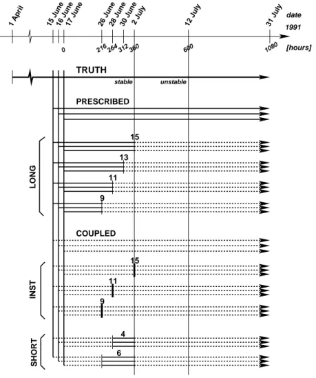
Fig. 2. Schematics of the set of numer-ical experiments with coupled and un-coupled soil/atmosphere components. The upper thick arrow shows the deter-ministic reference simulation TRUTH. All other experiments are 3-member spin-off ensembles from TRUTH (rep-resented by a set of 3 arrows). For pe-riods in which the model is run in the coupled (uncoupled/prescribed) mode, arrows or arrow sections are shown with a dotted (solid) line.

1 April 1991, 00:00 UTC, and ended on 31 August 1991. It is represented by the topmost thick arrow in Fig. 2. The ERA reanalysis provides its initial atmospheric conditions as well as its lateral boundary conditions. Its initial soil conditions on 1 April were taken from the National Center for Environ-mental Prediction (NCEP), rather than the ERA reanalyses (Kalnay et al., 1996) for consistency with previous experi-ments (see Heck et al. (2001) for a discussion of these con-siderations).

In order to assess the influence of the soil conditions upon predictability, ensemble simulations with 3 members are per-formed using different degrees of soil/atmosphere coupling. The respective ensemble members are driven by the same lat-eral boundary conditions as TRUTH, and in effect, they try to reproduce TRUTH. Figure 2 shows a schematics of the set of experiments. Each arrow represents an individual in-tegration. Solid arrows, or arrow sections, designate periods in which the ensemble members are in the prescribed mode, reading all soil variables from TRUTH. Dotted arrows, or ar-row sections, designate those periods in which the soil model is coupled to the atmosphere model.

The first two ensembles, referred to as COUPLED and PRESCRIBED, are carried out in the coupled and prescribed

modes, respectively, for the entire duration of the simulation. They are generated by perturbing the TRUTH’s atmosphere in the following manner: the initial atmospheric conditions are borrowed from the ECMWF reanalysis on 3 consecu-tive days, 15, 16, and 17 June, while the soil conditions of TRUTH are left untouched for those days. The two ensem-bles cover 1.5 months and ended on 31 July 1991.

The LONG ensembles are a variation of PRESCRIBED. They are identical to PRESCRIBED in an initial period, but the soil-atmosphere coupling is switched on after 15, 13, 11, and 9 days, respectively. The individual ensembles are named after the length of the prescribed phase, i.e. LONG15 is uncoupled over the first 15 days, from t=0 to t=360 h. LONG13 is in the prescribed mode between t=0 and t=312 h, LONG11 is between t=0 and t=264 h, and LONG9 is be-tween t=0 and t=216 h.

The INST and SHORT ensembles are variations of COU-PLED. In INST, the soil variables of the COUPLED simula-tion are corrected to the values of TRUTH at one instant, af-ter which the model is returned to the coupled mode. This is done at precisely 15, 11, and 9 days into the COUPLED sim-ulation. The instantaneous uncoupling is indicated in Fig. 2 by a thick bar intersecting the arrows. The instants chosen

for the forcing are t=360 h (INST15), t=264 h (INST11), and t=216 h (INST9).

Finally, in the third set of ensembles, referred to as SHORT, the soil values from TRUTH are continuously pre-scribed over a short period of 4 and 6 days, immediately fol-lowing the first 11 and 9 days of COUPLED, respectively. The soil-atmosphere coupling is subsequently switched on again until the end of the simulation. Thus, the forcing takes place during 4 days between t=264 h and t=360 h (SHORT4), and 6 days between t=216 h and t=360 h (SHORT6), respec-tively.

The selected ensemble methodology calls for two com-ments. First, the method for generating the ensemble, chosen for its simplicity, will lead to large initial differences between ensemble members and TRUTH, as if the simulations were initialized with analyses that are mediocre in the interior of the domain, while perfect at the lateral boundaries. This somewhat unusual trait, however, is not expected to have any bearing upon the results of this study, since the atmospheric evolution during the first 10 to 15 days of the simulation is deterministically controlled by the lateral boundary condi-tions (see Sect. 4). Second, the size of the ensemble is quite small (3 members). To test the sensitivity of the results with respect to a larger ensemble size, we have conducted 3 addi-tional integrations for the COUPLED ensemble, which is the ensemble with the largest spread. The results suggest that the predictability characteristics of the system are well captured by the small 3-member ensemble, although the small size of the ensemble remains a limitation to our study.

2.3 Employed error measures

To analyze the simulations, standard error scores will be used in the following way. Let χk(i, j, tn)be the value of

a given variable of the member k of a K-member ensemble at grid-point (i, j ) and time tn, ¯χ (i, j, tn)its ensemble mean,

and χT(i, j, tn)the respective value of TRUTH. The

over-all quality of an ensemble simulation will be assessed by the ensemble-mean root-mean square (RMSE) error with respect to TRUTH, i.e. δ(tn) = 1 K K X k=1 RMSEk(tn) = 1 K K X k=1 q < (χk(i, j, tn) − χT(i, j, tn))2>, (1)

where < > represents the domain mean taken over all (i, j ) grid-points.

If χkand χT are expressed as anomalies with respect to the

time-average [χT] = _N1 PNn=1χT(i, j, tn)of TRUTH, the

mean squared error (MSE) of χkcan be decomposed

accord-ing to Murphy and Epstein (1989) to reveal the individual contributions of the error in the mean anomaly (first term), the error in the variability (second term), and the error in the spatial pattern (third term):

MSEk(tn) = (< χk0 > − < χ 0 T >)2+(sχ_k0 −sχ_T0)2 +2(1 − r_χ0 kχ 0 T)sχ 0 ksχ 0 T, (2)

where χ_k0 = χk− [χT], χ_T0 = χT − [χT], s is the spatial

standard deviation, and r the spatial correlation coefficient. The predictability will be assessed by the ensemble spread defined as σ (tn) = 1 K K X k=1 q < (χk(i, j, tn) − ¯χ (i, j, tn))2>. (3)

It corresponds to the ensemble-mean RMS error with respect to the ensemble mean.

3 Truth: validation with respect to the ERA reanalysis

Although TRUTH is assumed to be reality and should not be questioned as such, it is interesting at this point to ex-amine its performance with respect to its driving ECMWF reanalysis. Indeed, it displays a distinct period in the midst of the integration, during which the atmospheric evolution is very poorly predicted, despite the continuous forcing with true lateral boundary conditions. As we shall see later, the behaviour during this period will constitute an important cri-terion in evaluating the ensemble experiments carried out to reproduce TRUTH.

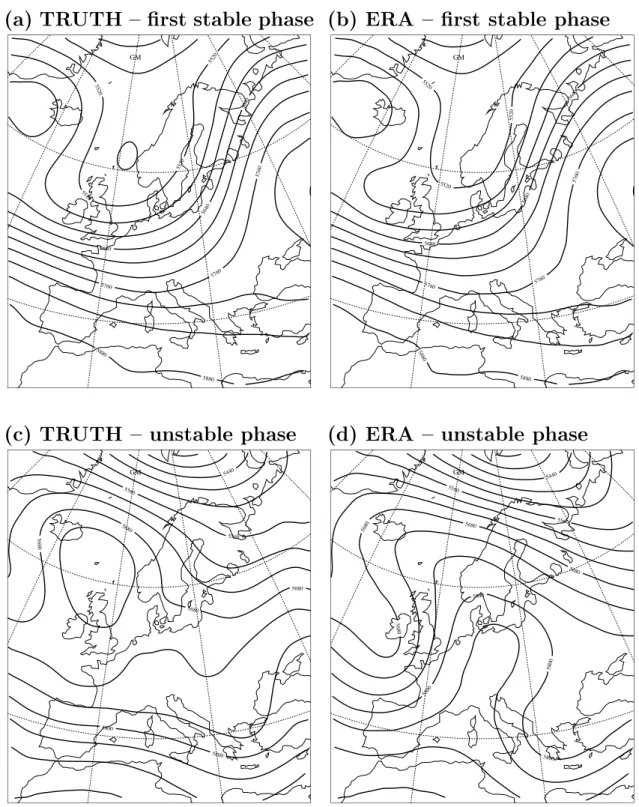
The evolution of the root mean square (RMS) error of TRUTH with respect to the reanalysis, averaged over the whole computational domain (see Fig. 1), is shown for the 850 hPa temperature field and the 500 hPa geopotential height in Figs. 3a and 3b, respectively. It reveals a “sta-ble” initial phase of about 15 days in duration (hours 0 to 360 of the simulation), during which the RMS errors are only 30 gpm for the 500 hPa geopotential height, and below 2 K for the 850 hPa temperature. Compared to current day ECMWF forecasting scores over Europe, these errors corre-spond to the mean error of a 2-day forecast. This stable and predictable phase is followed by a 10-day “unstable” phase (hours 360 to 600) during which the error rises abruptly to 120 gpm for the geopotential height and to nearly 5 K for the temperature field. During this period, from a practical point of view, the predictions are useless. Thereafter, in a second stable phase, the error stabilizes anew around the av-erage value it had at the beginning of the simulation. For comparison, the persistence of the reanalysis with respect to the first time in the diagram (17 June 1991, 00:00 UTC) is also indicated, and this suggests that the unstable phase is associated with a transition into a very different flow regime. A glance at the geopotential height contours at 500 hPa, averaged over the first 15 days (Figs. 4a and 4b), reveals that the simulated mean pattern is extremely close to that of the reanalysis. The following 10-day unstable phase, on the other hand, is characterized by weak advection in the south-ern half of the domain. As a result, there is a higher error level leading to striking differences between the patterns of the respective mean 500 hPa geopotential heights (Figs. 4c and 4d). This suggests that the evolution of the dynamical fields is only partly deterministically controlled by the lateral

(a) T at 850 hPa[K]

[hours]

(b) Z at 500 hPa[gpm]

[hours]

Fig. 3. Validation of TRUTH with respect to ERA: domain-averaged root mean square error for (a) the 850 hPa temperature field [K], and (b) the 500 hPa geopotential height [gpm]. For com-parison, the persistence of the reanalysis with respect to the first day of the simulation (17 June 00:00 UTC) is displayed with a dotted line.

boundaries between t=360 and t=600. Thus, an ensemble simulation that seeks to reproduce TRUTH with a limited-area model during this time period can be expected to exhibit large uncertainty and ensemble spread.

It should be noted, however, that our choice of TRUTH as reference weather evolution, despite its poor performance during the unstable phase, does not constitute a handicap: as

we shall see below, a sufficiently large ensemble would cer-tainly include at least one member close to the observations, even during the unstable phase.

4 Coupled vs. prescribed

The predictability of the weather over the time span under consideration is investigated using coupled and uncoupled ensemble integrations. The first ensemble, COUPLED, of-fers knowledge of the “natural” predictability under conven-tional, coupled conditions. The second ensemble, PRES-CRIBED, makes use of the uncoupled or prescribed mode, continuously providing the atmosphere with the correct and accurate soil conditions of TRUTH. Since it is assumed to perfectly simulate reality, the analysis of all experiments is carried out with respect to TRUTH; henceforth, the deviation of the dynamical fields of a given experiment from TRUTH will simply be referred to as its “error”. Recall that COU-PLED, PRESCRIBED, and TRUTH are driven by the same lateral boundary data from ERA, but TRUTH is initialized much earlier.

Figure 5 shows the 500 hPa geopotential height RMS er-ror of the COUPLED and PRESCRIBED ensembles. In Figs. 5a and 5b, the individual members of the two experi-ments are represented, while the ensemble means are com-pared in Fig. 5c (note the difference in vertical axis scale with Fig. 3). In both the COUPLED and PRESCRIBED ensembles, the initial difference from TRUTH is compara-tively large, about 40 gpm at the beginning of the simula-tion, reflecting the differences between the ECMWF reanal-ysis and TRUTH. For both ensembles, the RMS differences rapidly decrease to ∼ 10 gpm following initialization, and then remain approximately constant during the rest of the first 15 days for all three members of the respective ensem-bles, thus reflecting the strong deterministic control of the evolution by the lateral boundaries during this phase. The better performance in terms of COUPLED versus TRUTH, than in terms of TRUTH versus ERA, simply demonstrates that our model finds it easier to reproduce its own simulation than an observed evolution. During the subsequent unsta-ble phase, however, the members of the COUPLED ensem-ble display consideraensem-ble spread. Even an ensemensem-ble of such modest size produces both a member very close to TRUTH, and one close to the reanalysis (the member with the largest difference from TRUTH). The largest error during this time period is about 60 gpm, i.e. half the error of TRUTH with respect to the reanalysis. Following the unstable phase, the 3 members’ curves converge again at an RMS difference of ∼10 gpm with respect to TRUTH. Unlike COUPLED, the members of the PRESCRIBED ensemble remain close to TRUTH throughout the period, including the unstable phase. The temperature field at 850 hPa yields, in essence, the same evolution as the geopotential height, and will, therefore, no longer be considered.

Before proceeding with the discussion, the notion of pre-dictability in a limited-area model is briefly recalled.

Pre-(a) TRUTH { rst stable phase (b) ERA { rst stable phase 5520 5520 5520 5520 5640 5640 5640 5760 5760 5760 5880 5880 GM 5520 5520 5520 5640 5640 5640 5760 5760 5760 5880 5880 GM

(c) TRUTH { unstable phase (d) ERA { unstable phase

5440 5560 5560 5680 5680 5680 5680 5800 5800 GM 5440 5560 5560 5680 5680 5680 5680 5800 5800 5800 5800 GM

Fig. 4. Validation of TRUTH with respect to ERA: time-average of the 500 hPa geopotential height over (a, b) the initial stable period (t=0 to 360), and (c, d) the unstable period (t=360 to 600), respectively, with the TRUTH (ERA) fields shown in the left-hand (right-hand) panels.

dictability in a regional model acquires a slightly different meaning than in a global model, since true information is continuously fed into the domain. The predictability in a re-gional model (the spread between ensemble members) will, therefore, not only depend on the nature and intensity of the initial perturbations, but also on the lateral boundary condi-tions. As discussed in Sect. 3, the unstable phase provides us

with an interesting period during which the lateral boundary conditions play a smaller role than usual, and during which there may be pronounced error growth in the interior of the model domain.

Comparison of the ensemble means of COUPLED and PRESCRIBED shows that their evolution can hardly be dis-tinguished during the two stable phases near the beginning

(a) RMSE COUPLED[gpm] (b) RMSE PRESCRIBED[gpm]

[hours] [hours]

(c) Ens. mean RMSE [gpm] (d) Ens. mean MSE Dec. [gpm

2 ]

[hours] [hours]

Fig. 5. Domain-averaged 500 hPa geopotential height RMS error [gpm] with respect to TRUTH for (a) the individual members of the COUPLED, and (b) PRESCRIBED ensemble integrations. The simulations initiated on 15, 16, and 17 June 1991 are represented by a solid, long-dashed, and dotted line, respectively. Panel (c) shows the corresponding evolution for the ensemble mean of COUPLED (solid line) and PRESCRIBED (long-dashed line), respectively. Panel (d) displays the ensemble mean MSE decomposition in mean anomaly error (solid), variability error (dot), and spatial pattern error (long-dash) for COUPLED (thick line) and PRESCRIBED (thin line), in [gpm2].

and end of the integration. The RMS errors are almost iden-tical, despite the surplus of true soil information fed into the PRESCRIBED ensemble. Evidently, the forcing with soil variables has no significant influence upon the atmo-spheric evolution during these phases. However, 3 days be-fore the end of the first stable phase (t=360, 15 days into the simulation), a distinct bifurcation occurs within the COU-PLED ensemble, with one of the ensemble members exhibit-ing an RMS error of up to ∼ 60 gpm. The ensemble mean of

the Murphy-Epstein MSE decomposition for COUPLED and PRESCRIBED shown in Fig. 5d reveals that the bifurcation can essentially be attributed to a divergence in the spatial pat-tern. Since the error of the PRESCRIBED ensemble, as well as its spread, remains very small even during this period, we can conclude that the land-surface forcing plays a decisive role in this process.

Further aspects of the nature of the soil/atmosphere cou-pling in the ensembles are provided in Fig. 6 , where we focus

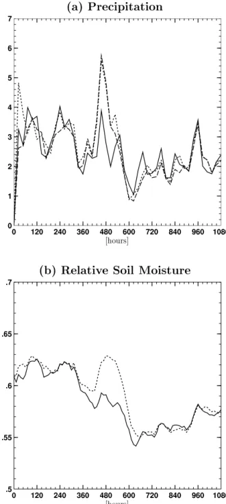
upon the ensemble member initialized on 17 June 00:00 UTC (which produced the largest errors in the COUPLED ensem-ble). The time traces of precipitation and the relative soil moisture content in the upper 10 cm of the soil are shown in Figs. 6a and 6b, respectively, both averaged over the land grid-points of the domain for TRUTH (dotted line), COU-PLED (solid) and PRESCRIBED (long-dashed). In the pre-cipitation field, the bifurcation at the end of the stable phase is clearly visible, resulting in an underestimation of domain-averaged precipitation of almost 20%. The differences in the accumulated precipitation pattern during the unstable phase (not shown) are essentially located over land and in the cen-tral band of the domain, where the patterns of mean geopo-tential height signal large discrepancies between TRUTH and ERA (Fig. 4). The PRESCRIBED simulation, on the other hand, follows TRUTH faithfully until the end of the simula-tion, and the respective precipitation patterns, even during the unstable phase, are nearly identical. From the middle to the end of June, which represents the first stable phase of the sim-ulation, the relative soil moisture content of both COUPLED and TRUTH is a little above 60% of the pore volume, step-ping down to 55% for the last three weeks of July. The transi-tion between these two values occurs during the unstable pe-riod, and clearly illustrates the effect of the bifurcation. The TRUTH soil moisture experiences a sudden, strong increase in the midst of its descent, while the soil moisture of the COUPLED simulation, receiving a more modest supply of precipitation, continuously decreases. Thus, the difference in soil moisture between COUPLED and PRESCRIBED, both in temporal evolution and in geographical distribution (not shown), is mirrored in the differences between the precipita-tion fields.

Figure 7 depicts the ensemble-mean vertical distribution of the error of COUPLED and PRESCRIBED with respect to TRUTH for the temperature and specific humidity, aaged over the land grid-points of the full domain. The ver-tical profile of the temperature bias (Fig. 7a) shows that the deviation from TRUTH is quite homogeneous throughout the troposphere. This remarkable feature is present in all mem-bers of the two ensembles, both in the stable and the unstable phases, despite the large spread within the COUPLED en-semble during the unstable phase (not shown). Thus, both for PRESCRIBED and for COUPLED, the error generated during the unstable phase is not confined to one particular layer of the troposphere. The COUPLED ensemble mean tends to overestimate the TRUTH tropospheric temperature, while the PRESCRIBED ensemble is associated with a (sub-stantially smaller) temperature underestimation. In contrast, during the stable phase (not shown), both PRESCRIBED and COUPLED slightly underestimate TRUTH, and differ from one another by less than 0.1 K. The specific humidity profiles (Fig. 7b) show a compatible response, i.e. overestimation of humidity with positive temperature bias, and vice versa.

In summary, the ensemble integrations have served to identify two regimes of the regional weather evolution. Dur-ing the stable phases, the predictability of the regional weather evolution is only marginally affected by the soil.

(a) Precipitation

[hours]

(b) Relative Soil Moisture

[hours]

Fig. 6. Evolution of (a) precipitation [mm/24 h] and (b) relative soil moisture content of the upper 10 cm of COUPLED (solid line), PRESCRIBED (long-dashed line), and TRUTH (dashed line). For both ensembles, only the member starting on 17 June 1991 are rep-resented, and the spatial averaging covers all land-points of the do-main. Since the TRUTH and PRESCRIBED simulation have, by definition, the same soil variables, only the former is visible in (b).

Surprisingly, the stipulation of correct information at the lower boundary, as in PRESCRIBED, does not lead to an improvement of predictability. In contrast, however, dur-ing the unstable phase, the soil is somehow involved in the weather evolution. The COUPLED ensemble is

character-(a) Temperature

[K]

(b) Specic Humidity

[g/kg]

Fig. 7. Vertical distribution of the ensemble-mean land-points domain-mean bias with respect to TRUTH for (a) temperature [K] and (b) specific humidity [g/kg]. The two ensembles COUPLED and PRESCRIBED are shown with solid and dashed lines, respec-tively.

ized by a large spread (bifurcation) between the ensemble members, and the underlying processes involve pronounced differences in precipitation and soil moisture content, and extend throughout the troposphere. In the PRESCRIBED mode, we strongly interfere with the chaotic evolution of the

entire system. The differences between the PRESCRIBED and COUPLED ensembles do not reveal the mechanism of the underlying bifurcation (which is presumably driven by the chaotic nature of atmospheric circulation), but they demonstrate the heavy involvement of the soil in this pro-cess. In particular, forcing the simulations with the correct soil moisture and temperature evolutions (as done in PRE-SCRIBED), drastically decreases the spread of the ensemble, thereby suppressing the respective bifurcation seen in COU-PLED, and ultimately yielding a nearly correct precipitation response, both in its distribution in space and in time.

5 Variations in soil forcing: long, short, and instanta-neous forcing periods

The two previously discussed ensemble integrations reveal the effect of permanent coupling or uncoupling of the at-mosphere/soil systems upon predictability. Provided with perfect soil conditions, the PRESCRIBED ensemble faith-fully reproduced TRUTH, and indeed, viewed the unstable phase as a predictable period. Yet it raises a few intriguing questions. In particular, since we are dealing with a chaotic system, the success of prescribing the soil variables does not necessarily imply that the observed bifurcation in COU-PLED is related to coupled atmosphere/soil interactions. In-stead, prescribing the soil might just help to guide the at-mospheric trajectory in phase-space along its true evolution, thus avoiding the bifurcation into a neighbouring region of phase-space. If this is the case, we would like to know – from a forecasting point of view where the prescribed mode is not a valid option – whether prescribing the soil just prior to the beginning of the unstable phase improves a subsequent cou-pled forecast. In other words, how would the system evolve if the integration were switched back from the prescribed to the coupled mode? Can the land-surface forcing rectify the evolution of the atmospheric dynamical fields, and if so, what is the minimum prescribed period that needs to be applied? To address these issues, three further sets of ensemble exper-iments were conducted.

5.1 Long prescribed phase (9–15 days)

The LONG ensembles examine the extent to which the pos-itive impact of the land-surface forcing persists after re-establishing the soil-atmosphere interaction. They involve long periods (many days) in the prescribed mode, followed by coupled integrations. The long forcing period mimics the effects of a soil data assimilation system upon a sub-sequent coupled ensemble simulation. Figure 8a compares the 500 hPa geopotential height ensemble-mean RMS error of the four LONG experiments. The ensembles prescribed over the first 15, 13, 11, and 9 days (LONG15, LONG13, LONG11, and LONG9), are represented by a solid, long-dashed, long-dashed, and dotted line, respectively. The LONG ensembles deviate from one another no earlier than at the on-set of the unstable phase (which begins on day 15, t=360),

(a)RMSE LONG (b) SpreadLONG

[gpm]

[hours] [hours]

(c) RMSE INST (d) RMSESHORT

[gpm]

[hours] [hours]

Fig. 8. Domain-averaged 500 hPa geopotential height RMS error [gpm] for the ensemble-means of (a) all LONG ensembles, (c) all INST en-sembles, and (d) all SHORT ensem-bles. In these panels, the ensemble mean RMS error for COUPLED (PRE-SCRIBED) are plotted for comparison with a thin solid (thin, long-dashed) line. Panel (b) shows the spread of the LONG ensembles. The individ-ual ensembles are coded with the fol-lowing line styles: solid for LONG15, INST15 and SHORT4; long-dashed for LONG13, INST11, SHORT6; dashed for LONG11, INST9; and dotted for LONG9.

despite switching to the coupled mode at progressively ear-lier dates prior to the beginning of the unstable phase. Yet, remarkably enough, prescribing the lower boundary of the at-mosphere over 13 or 15 days (nearly the entire stable phase) successfully maintains the atmosphere very close to TRUTH throughout the unstable phase, and beyond! Even reducing the forcing period to 11 or 9 days strongly attenuates the er-ror growth during the subsequent unstable period.

An estimation of the ensemble spread within each of the LONG ensembles and, therefore, of the predictability of the system, can be derived from the ensemble-mean RMS error with respect to the individual ensemble means (rather than with respect to TRUTH, see Sect. 2.3). This quantity is rep-resented in Fig. 8b for each of the LONG experiments with the same conventions as in Fig. 8a. For comparison, the dis-persion of the COUPLED ensemble is also included as a thin solid line. Obviously, the spread of all LONG ensembles is considerably reduced, especially for LONG15, LONG13, and LONG9; only LONG11 stands out with a comparatively large dispersion. This points towards an improvement in dictability during the unstable phase as a result of the pre-ceding soil forcing. Indeed, contrary to the ensemble mean error, which showed a steady increase with an earlier transi-tion to the coupled mode (Fig. 8a), three of the four LONG

experiments show a spread which is almost unaffected by the presence of the unstable period.

The LONG experiments thus clearly show the positive im-pacts of a perfect soil-moisture and soil-temperature data as-similation system. The benefits from such a system have a long persistence and may have a positive impact even several days after returning to a coupled forecasting mode.

5.2 Instantaneous forcing

The INST ensembles investigate whether the course of the dynamic evolution of the coupled system is affected by the instantaneous injection of correct soil conditions. Except for this instantaneous injection of land-surface information, the entire simulations are conducted in the coupled mode. Fig-ure 8c illustrates the evolution of the ensemble-mean 500 hPa RMS error. The three ensembles, INST15, INST11 and INST9, instantaneously forced at day 15, 11, and 9 of the simulation, are represented by a solid, long-dashed, and dot-ted line, respectively. For comparison, the RMS error of the COUPLED (thin solid line) and PRESCRIBED (thin dashed line) ensembles are also included in the figure.

Evidently, injecting perfect soil variables at a given instant brings no significant improvement to the dynamic evolution of the atmosphere. In the case of INST15, the soil

informa-tion is injected when the unstable phase begins (15 days into the simulations), but the results cannot be distinguished from the COUPLED ensemble with the naked eye. Even injection at an earlier time, such as 4 days (INST11) or 6 days (INST9) before the onset of the unstable phase only leads to marginal differences. All of the INST ensembles can barely be dis-tinguished from the fully coupled simulation. This serves to demonstrate that the impetus towards the bifurcation within COUPLED is not present in the soil, but rather in the atmo-sphere. The benefits of prescribing the soil conditions is to guide the atmospheric trajectory in phase-space along its true evolution, and thereby avoid the bifurcation into neighboring phase-space.

5.3 Short forcing (4–6 days)

Evidently, long forcing (as in LONG) has a pronounced im-pact upon the subsequent evolution of the coupled system, while instantaneous forcing (as in INST) is virtually with-out effect. The last set of ensembles, referred to as SHORT, is designed to identify the minimal time period needed to benefit from soil forcing. To this end, the soil is prescribed for a short time period immediately preceding the begin-ning of the unstable phase. Figure 8d shows two such en-semble experiments that employ prescribed soil conditions during 4 days (SHORT4, solid line) and 6 days (SHORT6, long-dashed line). Both experiments yield some error reduc-tion and attenuate the deviareduc-tion from TRUTH, but the effect is substantially less pronounced than in the LONG experi-ments. Strangely enough, the 6-day forcing produces worse results than the 4-day forcing, presumably a consequence of the (too) small ensemble size.

To conclude this subsection, there is strong evidence that for land-surface forcing to become notable within our test-ing framework, a forctest-ing period of about 10 days is optimal. Shorter forcing periods are only partly able to correct erro-neous weather evolutions.

6 Discussion and conclusion

In the present study, we have conducted several ensemble ex-periments to test the sensitivity of atmospheric predictabil-ity with respect to the coupling or uncoupling of the land-surface/atmosphere systems. The validation of the experi-ments was conducted with respect to a reference simulation that plays the role of reality and was referred to as TRUTH. Since this reference weather evolution was generated with the same (coupled) model, the study corresponds to conduct-ing predictability experiments by assumconduct-ing the existence of a perfect, error-free model. The issue of model error is there-fore not addressed.

The model utilized is a regional climate model, which is continuously driven at its lateral boundaries by the ECMWF reanalyses. This methodology, in effect, assumes that the in-cident baroclinic eddies are known, thus allowing us to focus upon the predictability of the soil/atmosphere system within

a specific domain. Without this continuous lateral boundary forcing, it would be more difficult to pinpoint the soil’s rele-vance.

The weather episode under investigation, a 45-day period during the summer of 1991, was shown to be character-ized by “stable” and “unstable” phases, which exhibit drasti-cally different behaviour in terms of predictability. The pre-dictability in these phases was shown to intrinsically depend upon the mode (coupled or uncoupled) of the ensemble ex-periments. More specifically, during the two stable phases, predictability was very high (small ensemble spread) and, quite surprisingly, virtually identical for the coupled and un-coupled simulation modes. Thus, the prescription of the soil conditions did not improve the predictability in these stable phases.

In contrast, during the unstable phase of the time period, the relevant measures of predictability (500 hPa ensemble-mean error and ensemble spread) demonstrate that prescrib-ing the soil conditions leads to a significant improvement in the simulations, and in fact, is able to suppress a bifurcation that was observed in the coupled ensemble.

Prescribing the soil conditions throughout the entire sim-ulation implies continuously providing true information at the lower boundary of the atmosphere. Thus, the number of possible trajectories in phase-space is reduced, and it is, in principle, no surprise that the spread between ensemble members is reduced. Nevertheless, it is quite striking that prescribing the soil variables maintains the atmospheric evo-lution so close to TRUTH, and indeed spectacularly renders an unstable phase of the coupled ensemble predictable. Strik-ingly enough, the same result can be achieved even if pre-scribing the soil conditions is interrupted immediately prior to the unstable phase (as is done in the LONG ensembles). Additional experiments with shorter soil forcing periods fol-lowed by coupled integrations suggest that the soil forcing may guide the atmospheric phase-space trajectories along the true evolution of the system, but that it requires an extended time period of 10 to 15 days to realize its beneficial impact upon the ensemble behaviour. In particular, instantaneous updating of the soil, or short-term forcing over a few days, is not sufficient to rectify the evolution of the atmosphere.

Thus, over time scales of 10 to 15 days, the evolution of soil conditions can play an important role in the atmosphere’s evolution for summertime European conditions. This indi-cates that the re-initialization of soil moisture at regular in-tervals in a forecasting system, such as in a sophisticated data assimilation system, may have a greater influence on the dy-namical variables than expected. Indeed, the effects of such a procedure were shown to not only affect the lower tropo-spheric levels, but also reach higher up into the troposphere and lower stratosphere than is usually assumed, both in the coupled and uncoupled ensembles. This influence appears to be associated with altering the behaviour of the baroclinic systems, and not directly through other vertical exchange processes.

It must be emphasized at this point that the dramatic im-provement in predictability achieved by prescribing the

cor-rect land-surface evolution is to some extent related to the ideal conditions of the experiment, in which a perfect model is used, driven by perfect lateral boundary conditions and SSTs, and in which the exact values of TRUTH’s soil vari-ables are perfectly known. Any departure from these con-ditions would, therefore, imply an increase in degrees of freedom, and would no doubt reduce the ability of the land-surface states to influence the atmospheric evolution. Thus, the nature of our experiment is such as to maximize the role of soil moisture upon predictability. Follow-on experiments featuring a less perfect TRUTH could alleviate the depen-dence of the results upon a particular RCM. This could be done by both nudging TRUTH towards the ERA reanaly-ses during its entire 75-day simulation period, and forcing TRUTH’s land-surface scheme with observed precipitation.

The direct significance for medium-range weather fore-casting is more difficult to assess. In particular, while our experimental setup in experiments LONG and SHORT in-cludes a forcing of soil conditions (that mimics a soil assim-ilation system), a corresponding feature for atmospheric as-similation was not considered. In addition, the ensemble size was very small, and the time period encompasses a single episode of 45 days. Likewise, assessing the potential bene-fits of perturbing initial soil conditions in an ensemble pre-diction system would require additional experiments that in-clude systematic ensemble generation with atmospheric and soil perturbations of various amplitudes. In this sense, our conclusions are preliminary. Nevertheless, it is interesting to note that the coupling of the land and atmosphere systems has qualitatively a similar effect as that of coupling the at-mosphere with the ocean, namely to considerably increase the variability of the coupled system.

Acknowledgements. We are indebted to the German Weather

Ser-vice (DWD) and MeteoSwiss for providing the access to the nu-merical model. Special thanks are due to Detlev Majewski (DWD) and to Jean Quiby (MeteoSwiss) and their groups for technical sup-port. We are grateful to Daniel L¨uthi for valuable help in setting up the experiments, and to Pamela Heck, Christoph Frei, Pier-Luigi Vidale, and Andr´e Walser for numerous discussions and helpful ad-vice. We also would like to thank two anonymous reviewers for their constructive comments that have contributed towards improv-ing the final version of the paper. Finally, we would like to thank Mr. S. Fukudome for generously funding this research through the Nishinihon Institute of Technology in Kochi, Japan.

References

Beljaars, A. C. M., Viterbo, P., Miller, M. J., and Betts, A. K.: The anomalous rainfall over the United States during July 1993: Sen-sitivity to land surface parameterization and soil moisture, Mon. Wea. Rev., 124, 362–383, 1996.

Betts, A. K., Ball, J. H., Beljaars, A. C. M., Miller, M. J., and Viterbo, P. A.: The land-surface atmosphere interaction: a re-view based on observational and global modeling perspectives, J. Geophys. Res., 101, 7209–7225, 1996.

Buizza, R. and Palmer, T. N.: The singular-vector structure of the atmospheric global circulation, J. Atmos. Sci., 52, 1434–1456, 1995.

Christensen, O. B.: Relaxation of soil variables in a regional climate model, Tellus, 51A, 674–685, 1998.

Davies, H. C.: A lateral boundary formulation for multilevel predic-tion systems, Quart. J. Roy. Meteor. Soc., 102, 405–418, 1976. Dickinson, R. E.: Modeling evapotranspiration for

three-dimensional global climate models, Geophys. Monogr., 29, Mau-rice Ewing Volume 5, 58–72, 1984.

DWD: Dokumentation des EM/DM-Systems, (Ed) Schr¨odin, R. [Available from: German Weather Service, Zentralamt, 63004 Offenbach am Main], 1995.

DWD: Quarterly Report of the operational NWP-models of the Deutscher Wetterdienst, [Available from: German Weather Ser-vice, Zentralamt, 63004 Offenbach am Main], 1998.

Ehrendorfer, M. and Errico, R. M.: Mesoscale predictability and the spectrum of optimal perturbations, J. Atm. Sci., 52, 3475–3500, 1995.

Eltahir, E. A. B.: A soil moisture rainfall feedback mechanism. 1: Theory and observations, Water Resour. Res., 34, 765–776, 1998.

Findell, K. L. and Eltahir, E. A. B.: An analysis of the soil moisture-rainfall feedback, based on direct observations from Illinois, Wa-ter Resour. Res., 33, 725–735, 1997.

Frei, C., Sch¨ar, C., L¨uthi, D., and Davies, H. C.: Heavy precipitation processes in a warmer climate, Geophys. Res. Letters, 25, 1431– 1434, 1998.

Gibson, J. K., Kallberg, P., Uppala, S., Nomura, A., Hernandez, A., and Serrano, A.: ERA description, ECMWF Re-Analysis Project Report Series, Reading, UK, 1997.

Giorgi, F., Mearns, L. O., Shields, C., and Mayer, L.: A regional model study of the importance of local versus remote controls of the 1988 drought and the 1993 flood over the Central United States, J. Climate, 9, 1150–1162, 1996.

Heck, P., L¨uthi, D., Wernli, H., and Sch¨ar, C.: Climate impacts of European-scale anthropogenic vegetation changes: A study with a regional climate model. J. Geophys. Res., in press, 2001. Hu, Y., Gao, X., Shuttleworth, W. J., Gupta, H., Mahfouf, J.-F., and

Viterbo, P. A.: Soil-moisture nudging experiments with a single-column version of the ECMWF model, Quart. J. Roy. Meteor. Soc., 125, 1879–1902, 1999.

Jacobsen, I. and Heise, E.: A new economic method for the com-putation of the surface temperature in numerical models, Beitr. Phys. Atmos., 55, 128–141, 1982

Jones, R. G., Murphy, J. M., and Noguer, M.: Simulation of climate-change over europe using a nested regional-climate model, Part I: assessment of control climate, including sensitivity to location of lateral boundaries, Quart. J. Roy. Meteor. Soc., 121, 1413–1449, 1995.

Kalnay, E., Kanamitsu, M., Kistler, R., Collins, W., Deaven, D., Gandin, L., Iredell, M., Saha, S., White, G., Woollen, J., Zhu, Y., Chelliah, M., Ebisuzaki, W., Higgins, W., Janowiak, J., Mo, K. C., Ropelewski, C., Wang, J., Leetmaa, A., Reynolds, R., Jenne, R., and Joseph, D.: The NCEP/NCAR 40-year reanalysis project, B. Am. Meteorol. Soc., 77, 437–471, 1996.

Koster, R., Suarez, M., and Heiser, M.: Variance and predictabil-ity of precipitation at seasonal-to-interannual timescales, J. Hy-drometeor., 1, 26–46, 2000.

Laprise, R., Ravi Varma, M., Denis, B., Caya, D., and Zawadzki, I.: Predictability of a nested limited-area model, Mon. Wea. Rev., 128, 4149–4154, 2000.

L¨uthi, D., Cress, A., Davies, H. C., Frei, C., and Sch¨ar, C.: Inter-annual variability and regional climate simulations, Theor. Appl. Climatol., 53, 185–209, 1996.

Mahfouf, J. F.: Analysis of soil-moisture from near-surface param-eters – a feasibility study, J. Appl. Meteorol., 30, 1534–1547, 1991.

Majewski, D.: The Europa-Model of the Deutscher Wetterdienst. ECMWF Proc. “Numerical Methods in atmospheric models”, Reading, GB, 2, 147–191, 1991.

Molteni, F., Buizza, R., Palmer, T. N., and Petroliagis, T.: The ECMWF ensemble prediction system: methodology and valida-tion, Quart. J. Roy. Meteor. Soc., 122, 73–119, 1996.

Murphy, A. H. and Epstein, E. S.: Skill scores and correlation co-efficients in model verification, Mon. Wea. Rev., 117, 572–581, 1989.

Palmer, T. N.: Extended-range atmospheric prediction and the Lorenz model, B. Am. Meteorol. Soc., 74, 49–65, 1993. Pielke, R. A., Liston, G. E., Eastman, J. L., Lu, L., and Coughenour,

M.: Seasonal weather prediction as an initial value problem, J. Geophys. Res. – Atmos., 104, 19463–19479, 1999.

Rhodin, A., Kucharski, F., Callies, U., Eppel, D. P., and Wergen, W.: Variational analysis of effective soil moisture from screen-level atmospheric parameters: application to a short-range weather forecast model, Quart. J. Roy. Meteor. Soc., 125, 2427–2448, 1999.

Sch¨ar, C., Frei, C., L¨uthi, D., and Davies, H. C.: Surrogate climate

scenarios for regional climate models, Geophys. Res. Letters, 23, 669–672, 1996.

Sch¨ar, C., L¨uthi, D., and Beyerle, U.: The soil-precipitation feed-back: a process study with a regional climate model, J. Climate, 12, 722–741, 1999.

Seth, A. and Giorgi, F.: The effects of domain choice on sum-mer precipitation simulation and sensitivity in a regional climate model, J. Climate, 11, 2698–2712, 1998.

Shukla, J. and Mintz, Y.: Influence of land-surface evapotranspira-tion on the Earth’s climate, Science, 215, 1498–1501, 1982. Simmons, A. J. and Burridge, D. M.: An energy and

angular-momentum conserving finite-difference scheme and hybrid ver-tical coordinates, Mon. Wea. Rev., 109, 758–766, 1981. Van den Hurk, B. J. J. M., Bastiaanssen, W. G. M., Pelgrum, H., and

van Meijgaard, E.: A new methodology for assimilation of initial soil moisture fields in weather prediction models using Meteosat and NOAA data, J. of Appl. Meteorol., 36, 1271–1283, 1997. Viterbo, P. and Betts, A.: Impact of the ECMWF reanalysis soil

water on forecasts of the July 1993 Mississippi flood, J. Geophys. Res., 104, 19 361–19 366, 1999.

Weatherald, R. T. and Manabe, S.: The mechanism of summer dry-ness induced by greenhouse warming, J. Climate, 8, 3096–3108, 1995.