HAL Id: insu-01916927
https://hal-insu.archives-ouvertes.fr/insu-01916927
Submitted on 11 Mar 2019HAL is a multi-disciplinary open access archive for the deposit and dissemination of sci-entific research documents, whether they are pub-lished or not. The documents may come from teaching and research institutions in France or abroad, or from public or private research centers.
L’archive ouverte pluridisciplinaire HAL, est destinée au dépôt et à la diffusion de documents scientifiques de niveau recherche, publiés ou non, émanant des établissements d’enseignement et de recherche français ou étrangers, des laboratoires publics ou privés.
Past, Present and Future of Active Radio Frequency
Experiments in Space
A. V. Streltsov, Jean-Jacques Berthelier, A. A. Chernyshov, V. L. Frolov, F.
Honary, M. J. Kosch, R. P. Mccoy, E. V. Mishin, M. T. Rietveld
To cite this version:
A. V. Streltsov, Jean-Jacques Berthelier, A. A. Chernyshov, V. L. Frolov, F. Honary, et al.. Past, Present and Future of Active Radio Frequency Experiments in Space. Space Science Reviews, Springer Verlag, 2018, 214 (8), pp.118. �10.1007/s11214-018-0549-7�. �insu-01916927�
1
PAST, PRESENT AND FUTURE OF ACTIVE RADIO FREQUENCY EXPERIMENTS IN SPACE
A. V. Streltsov1,2, J.-J. Berthelier3, A. A. Chernyshov4, V. L. Frolov5,6, F. Honary7, M. J. Kosch7,8,9, R. P. McCoy10, E. V. Mishin11, M. T. Rietveld12,13
1Embry-Riddle Aeronautical University, Daytona Beach, Florida, USA;
2National Academy of Sciences at Space Vehicles Directorate, Air Force Research Laboratory,
Albuquerque, New Mexico, USA;
3LATMOS/IPSL, CNRS-UPMC-UVSQ, UPMC, Paris, France;
4Space Research Institute, Moscow, Russia;
5Nizhny Novgorod State University, Nizhny Novgorod, Russia; 6Kazan Federal University, Kazan, Russia;
7Lancaster University, Lancaster, United Kingdom;
8South African National Space Agency, Hermanus, South Africa;
9University of the Western Cape, Bellville, South Africa;
10Geophysical Institute, University of Alaska Fairbanks, Fairbanks, Alaska, USA;
11 Space Vehicles Directorate, Air Force Research Laboratory, Albuquerque, New Mexico, USA;
12EISCAT, Ramfjordbotn, Norway;
13UiT The Arctic University of Norway, Tromsø, Norway.
Abstract. Active ionospheric experiments using high-power, high-frequency transmitters, “heaters”, to study plasma processes in the ionosphere and magnetosphere continue to provide new insights into understanding plasma and geophysical proceses. This review describes the heating facilities, past and present, and discusses scientific results from these facilities and associated space missions. Phenomena that have been observed with these facilities are reviewed along with theoretical explanations that have been proposed or are commonly accepted. Gaps or uncertainties in understanding of heating initiated phenomena are discussed together with proposed science questions to be addressed in the future. Suggestions for improvements and additions to existing facilities are presented including important satellite missions which are necessary to answer the outstanding questions in this field.
Keywords. Active experiments. Ionospheric heating. HAARP. SURA. Arecibo. ULF waves. Ionospheric feedback instability. VLF waves. Ionospheric irregularities. Plasma instabilities. Wave-particle interactions. Artificial aurora. EISCAT. Ionosphere. DEMETER. Ionospheric resonator.
2 Acronyms
AA - anomalous absorption AGW - acoustic gravity waves AKR - auroral kilometric radiation API - artificial periodic irregularity ASE - artificially stimulated emissions
BF layer - the region of scattering from the bottom side F region BUM - broad upshifted maximum
BUS - broad upshifted structure BSS - broad symmetrical structure
CADI - Canadian Advanced Digital Ionosonde CNA - cosmic noise absorption
DL - descending layer
DM - downshifted maximum
DMSP - Defense Meteorological Satellite Program DP - downshifted peak
DSX - Demonstration and Science Experiments satellite DVH - descending virtual height
DW - diagnostic wave
EISCAT - European Incoherent SCATter Scientific Association EMIC - electromagnetic ion cyclotron wave
ERP - effective radiated power FAC - field-aligned current FAI - field-aligned irregularity
HAARP - High Frequency Active Auroral Research Program HIPAS - HIgh Power Auroral Stimulation observatory IAPD - Ion Acoustic Parametric Decay instability IAR - ionospheric Alfvén resonator
IDM - intermediate downshifted maximum IDV - ionosphere disturbed volume IFI - ionospheric feedback instability IRI - Ionospheric Research Instrument ISR - incoherent scatter radar
LH - lower hybrid
LSI - large-scale irregularity LT - Langmuir turbulence MI - modulation instability
MUIR - modular UHF ionospheric radar (at HAARP) MSI - medium-scale irregularity
MZ - magnetic zenith
NC - narrow continuum
NEIEL - naturally enhanced ion acoustic line OTHR - over-the-horizon radar
3 OTSI - oscillating two-stream instability PDI - parametric decay instability
PFISR - Poker Flat Incoherent Scatter Radar PL - plasma line
PMSE - polar mesospheric summer echoes PMWE - polar mesospheric winter echoes PPI - ponderomotive parametric instability
PW - pump wave
QPO - quasi-periodic oscillation SAPS - subauroral polarization stream SAID - subauroral ion drift
SEE - stimulated electromagnetic emission SLT - strong Langmuir turbulence
SSA - striction self-action SSI - small-scale irregularity SSSI - supra-small-scale irregularity SST - super strong (Langmuir) turbulence TEC - total electron content
TID - travelling ionospheric disturbance TPI - thermal parametric instability TSFI - thermal self-focusing instability
UH - upper hybrid
UHR - upper hybrid resonance UWE - upshifted wideband emission VPM - VLF and Particle Mapper satellite VPM - VLF and Particle Mapper satellite
WALES - weak-altitude extent ion line enhancements
4 Table of Contents 1 Introduction... 6 2 Experimental Facilities ... 8 2.1 Ground Facilities ... 8 2.1.1 HAARP ... 9 2.1.2 SURA ... 10 2.1.3 EISCAT ... 12 2.1.4 Arecibo ... 15 2.1.5 Science Topics ... 17 2.2 Satellites ... 18 2.2.1 DEMETER Satellite ... 20
2.2.2 Defense Meteorological Satellite Program (DMSP)... 22
2.2.3 The Demonstration and Science Experiments (DSX) Satellite ... 24
2.2.4 RESONANCE Satellite ... 26
3 Theory of the HF Ionospheric Modification ... 29
3.1 Propagation of O-Mode Waves ... 30
3.2 Electrostatic Plasma Waves ... 31
3.2.1 Wave-Particle Analogy ... 33
3.3 Ponderomotive Parametric Instability (PPI) ... 33
3.3.1 PPI in Isotropic Plasma (PPIL) ... 35
3.3.2 Parametric Decay Instability (PDIL) ... 36
3.3.3 Modulational Instability (MI) ... 36
3.4 PPI in the Plasma Resonance Layer ... 37
3.4.1 Strong Langmuir Turbulence (SLT) ... 38
3.4.2 Coexistence of WT and SLT Regimes ... 40
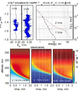
3.4.3 Full-Wave Simulations of SLT at HAARP ... 41
3.5 PPI in the Upper Hybrid Layer (PPIOUH /EB) ... 42
3.5.1 Upper Hybrid PPI ... 43
3.5.2 Langmuir Turbulence in the UH Layer ... 45
3.5.3 Lower Hybrid PPI ... 45
3.6 Nonlinear Thermal Effects... 46
3.6.1 Electron Heating and Thermal Flux... 47
3.6.2 Thermal Self-Focusing Instability (TSFI) ... 48
3.6.3 Thermal Parametric Instability (TPI) ... 48
3.7 Electron Acceleration ... 51
4 Active Experiments ... 53
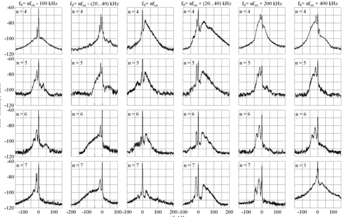
4.1 Stimulated Electromagnetic Emissions (SEEs) ... 53
4.2 Artificial Field-Aligned Irregularities (FAIs) ... 60
5
4.2.2 Temporal Development of FAIs ... 66
4.2.3 Relaxation of FAIs ... 67
4.2.4 Temporal Evolution of Short-Pulse Pumped FAIs ... 67
4.2.5 Spectral Characteristics of SSIs ... 68
4.2.6 Dependence of FAI Intensity on the Pump Power ... 70
4.2.7 Magnetic Zenith Effects ... 70
4.2.8 Unexplained UHF Radar Backscatter at the Magnetic Zenith ... 72
4.2.9 Gyroharmonic Effects Associated with FAIs ... 73
4.2.10 Concluding Remarks ... 76
4.3 Ducts ... 77
4.3.1 DEMETER Observations over SURA ... 78
4.3.2 DMSP and DEMETER Observations over HAARP ... 80
4.3.3 Numerical Modeling of Artificial Ducts ... 81
4.4 Optical Emissions ... 82
4.4.1 Artificial Aurora ... 82
4.4.2 Electron Temperature Effects ... 85
4.4.3 Magnetic Aspect Angle Effects ... 87
4.4.4 Electron Energy Spectrum ... 87
4.4.5 Small-Scale Optical Structures ... 88
4.4.6 X-Mode Optical Phenomena ... 89
4.4.7 Optical Phenomena in the E Region ... 90
4.4.8 Other phenomena ... 91
4.5 ULF/ELF/VLF Waves ... 91
4.5.1 Generation of ULF/ELF/VLF Waves ... 91
4.5.2 Resonant ULF Waves ... 97
4.5.3 ULF Waves in the Global Magnetospheric Resonator ... 99
4.5.4 ULF Waves in the Ionospheric Alfvén Resonator ... 102
4.5.5 ULF Waves in the Earth-Ionosphere Waveguide (Schumann Resonator) ... 103
4.5.6 ELF/VLF Waves in the Magnetosphere ... 105
4.6 Descending Artificial Ionization Layers (DLs) ... 107
4.6.1 Ionizing Wavefront ... 108
4.6.2 Observations of DLs ... 109
4.6.3 DL Theory ... 116
4.7 Other Active Experiments ... 121
4.7.1 Artificial Ionospheric Horizontal Periodic Irregularities (APIs) ... 121
4.7.2 E Region Ionospheric Perturbations ... 122
4.7.3 D Region and Mesospheric Perturbations ... 122
5 Conclusions... 124
6 Acknowledgements ... 127
6 1 Introduction
Active ionospheric experiments involving the use of high-power, high-frequency (HF) transmitters to heat small regions of the ionosphere have a tremendous potential to reveal a wealth of information about plasma processes. The Earth’s ionosphere is strongly coupled to the sun, less strongly coupled to the earth, is highly variable and exerts a wide array of effects on radio frequency (RF) propagation. Conventional ionospheric investigations involve remote sensing with RF transmitters on the ground or in space, or in-situ measurements with sounding rockets or satellites. To investigate a particular ionospheric phenomenon with conventional techniques, the experimenter must wait for that phenomena to appear. Active experiments can create a desired phenomenon on demand, effectively turning the overhead ionosphere into a plasma laboratory without walls.
This review is concerned with active experiments involving heating of the ionosphere with HF transmitters from the ground and does not address other classes of active experiments involving chemical releases or in-situ plasma discharges or beam injections. High-power, HF radio transmitters can disturb plasma in the Earth's ionosphere and magnetosphere providing a unique opportunity to study interaction between electromagnetic waves and particles without the limited spatial scale-size and chamber edge effects that can be encountered while performing plasma experiments in a laboratory. By modulating the transmitted power in time, space or frequency, the ionosphere can effectively become an antenna for the generation of lower frequency waves. These lower frequency waves (ELF, VLF, ULF) provide opportunities to study a wide array of electromagnetic wave-particle interactions. The resulting interaction between the EM “pump” wave and the ionospheric plasma can then be observed via a number of channels: UHF/VHF incoherent scatter radar measures the plasma density and temperature; optical instruments observe the visible-spectrum of optical emissions produced via suprathermal electron collisions with neutrals; radio receivers and spectrum analysers monitor the stimulated electromagnetic emission (SEE) signal emerging from the heated region.
The topic of active experiments by high power radio waves has generated enormous interest with thousands of publications including review articles by Gurevich [2007], Leyser [2001], and
Leyser and Wong [2009]. The focus of this review is to a) report on the theoretical and
experimental results from primarily the last decade in the areas of field-aligned irregularities, instabilities, ducts, ionization layers, optical emissions and ULF/ELF wave generation and propagation; b) discuss in detail satellite missions which have directly improved our understanding of new phenomena such as the formation of ducts; and c) to highlight science topics to be explored and propose experiments to address outstanding questions in this field.
Section 2 describes the experimental facilities with section 2.1 giving a brief history and details of the four currently active ground-based heaters together with their main diagnostic instruments. Satellites and rockets have provided unique and important in-situ measurements of the heated volume and disturbances propagating from it to the upper ionosphere and magnetosphere. They are mentioned in some of the sections describing each HF facility. The most recent and planned
7
satellites, which are an increasingly important space-based diagnostic of HF ionospheric pumping above all the HF facilities, are described separately in section 2.2.
Ideally heating experiments should be specially designed to test specific hypotheses. This requires a quantitative and comprehensive modelling of linear and nonlinear aspects of wave propagation, wave-wave and wave particle interactions, turbulence and instabilities of many different types in a highly inhomogeneous magnetized plasma. To make this review as self-consistent as possible, we include in section 3 an overview of the various physical mechanisms that are involved in the most important observed phenomena related to ionospheric heating.
Section 4 reviews recent advances in the ionospheric heating experiments focusing on generation and spatio-temporal properties of 1) stimulated electromagnetic emissions (SEE), 2) artificial ionospheric structures or magnetic field-aligned irregularities (FAI), 3) ducts, 4) optical emissions, also known as artificial aurora, 5) ULF and ELF waves propagating into the magnetosphere and in the earth-ionosphere waveguide, 6) artificial ionization layers.
The conclusions section summarizes the current state of knowledge in the field of ionosphere heating with HF waves of different powers and provides a suggested list of problems to be addressed in the future.
8 2 Experimental Facilities
2.1 Ground Facilities
The first active ionospheric experiment occurred unintentionally when the broadcast from a powerful commercial AM station in Luxembourg could be heard by a receiver tuned to another medium frequency station [Tellegen, 1933]. This “cross modulation”, now known as the “Luxembourg Effect”, is explained by as little as a 5% change in electron temperature caused by the powerful modulating station, which modifies the electron collision frequency and hence the absorption of other radio waves traveling through the disturbed region which ultimately superimposes the modulation on them.
The first major HF facility constructed was a 1.45 MHz transmitter near Moscow, Russia which was built to test a hypothesis published by Bailey [1937] that HF radio wave energy at the electron gyro frequency could efficiently accelerate electrons into atomic oxygen atoms to produce visible light. Experiments were performed in 1961 and were not successful, but since the work was highly classified, it was not until it was unclassified in 1973 that researchers were able to explain why the optical emissions were not possible [Gurevich, 2007].
High power ionospheric modification research first appeared in the open literature using experiments in Platteville, USA led by W. Utlaut. Findings were collected in a special issue of
Radio Science, vol 9, 1974, based on HF heater induced spread F, field-aligned ionization
structure, wide-band absorption, and airglow. It soon became clear that it would be highly desirable to include an incoherent scatter radar in the complement of diagnostic tools. This led to an ionospheric heater being introduced at Arecibo by suspending an HF feed above the primary reflector allowing the 433 MHz incoherent scatter facility to be used to probe the heating effects [Gordon et al., 1971]. Several other relatively low power facilities were subsequently built during the 1970’s, such as Monchengorsk, near Murmansk, and Zimenki, near Nizhny Novgorod, Russia.
The present modern class of heater facilities were then built, one at the high latitude location of Tromsø, Norway, co-located with the two new EISCAT incoherent scatter radars (ISR) in 1981, and the other at the mid-latitude station, SURA, in Russia. Another high latitude station, HIPAS, was built by the University of California in Alaska [Wong et al., 1990] in the late 1980’s and operated from 1986 to 2007. In 1993 the High Frequency Active Auroral Research Program (HAARP) facility was started, reaching completion in 2007 making it the most powerful and advanced facility of all. The highest latitude heater, SPEAR [Robinson, 2006], was built on the island of Spitsbergen and operated from 2004 to 2015, but has since been dismantled.
Today there are four active HF facilities around the world. They are: SURA in Russia [Belikovich et al., 2007], EISCAT heating facility (built and formerly operated by Germany's Max-Planck Institute) in Norway [Rietveld et al., 2016], HAARP in Alaska, USA [Pedersen and
Carlson, 2001], and most recently a new HF facility for the Arecibo 300 m antenna [Carlson et al., 2017]. Only Arecibo and the EISCAT HF facilities are co-located with incoherent scatter
radars, although HAARP has a small UHF phased array radar called the Modular UHF Ionospheric Radar (MUIR) which can receive HF-enhanced echoes normally seen with ISRs. In section 2.1
9
these four facilities are described in more detail together with an outline of the major ground-based diagnostics and the research areas these facilities address.
In addition to dedicated HF facilities designed specifically for interactions with the ionosphere, it should not be forgotten that other powerful radio transmitting facilities like ISRs are also capable of heating thermal electrons in spite of their frequencies being much higher than HF. The mechanism is simple Ohmic heating in the collisional lower ionosphere, by the extremely powerful ISR transmissions. This was demonstrated using the Arecibo facility by Sulzer et al. [1982], and will also be possible with the new EISCAT_3D facility under construction in northern Scandinavia [McCrea et al., 2015].
2.1.1 HAARP
The High frequency Active Auroral Research Program (HAARP) facility, located in Gakona, Alaska (latitude: 62.39° N, 145.15° W; magnetic latitude: 63.09° N, 92.44° W) is the world’s most powerful and sophisticated facility for active experimentation in the upper atmosphere and ionosphere. HAARP uses powerful HF waves to heat small (~30-100 km) regions of the upper atmosphere to stimulate particular geophysical processes that can be disentangled by ground-based diagnostic instruments from complex and coupled natural phenomena in the thermosphere and ionosphere. The HAARP facility can indeed create its own natural plasma laboratory without walls in the ionosphere and perform controlled experiments to study a variety of linear and nonlinear plasma physics phenomena that are difficult to capture with satellites or sounding rockets.
HAARP is ideally located to investigate a large variety of geophysical phenomena. The overhead sub-auroral ionosphere can be stable but during even moderately active geomagnetic conditions, the active auroral zone moves above HAARP allowing experiments to be performed within the aurora. Near an L-shell of 5, low frequency waves generated by HAARP can propagate upward along magnetic field lines high into the magnetosphere and even into the conjugate ionosphere.
The primary HAARP transmitter is the Ionospheric Research Instrument (IRI), a phased array of 180 HF crossed dipole antennas covering an area of 33 acres and radiating EM waves in the frequency range 2.8 to 10 MHz with a net power of 3.6 MW. The antenna array is fed by transmitters located in 30 electronic shelters (trailers) powered by five 2500 kW generators, each driven by a 3600 hp diesel engine (4 + 1 spare). The multiple beams from the phased array can be rapidly reconfigured to achieve
Figure 2.1. HAARP antenna array. Drone photo courtesy of
10
complex spatially and temporally variable antenna patterns down to elevations angles of 30º from the zenith. A photo of the antenna array is shown in Figure 2.1. Because HAARP employs a phased array antenna, energy can be concentrated along variable directions, producing an effective radiated power (ERP) in the few GW range allowing a wide range of unique experiments. Other key instruments at HAARP include an ionosonde, GPS receivers, magnetometers, riometers, optical instruments and the MUIR radar.
The HAARP program was initiated in 1989 and managed by the Air Force Research Laboratory (AFRL) and the Office of Naval Research (ONR). The facility was enhanced with additional funding from the Defense Advanced Research Projects Agency (DARPA), AFRL and ONR. In 2007 HAARP began operating at its current power levels. The ONR interest for HAARP was primarily focused on making the heated ionosphere a many-kilometer long antenna to generate and propagate extremely low frequency (ELF) signals for submarine communications. AFRL interest included studies of over the horizon radar capabilities and using the ionosphere to generate and inject ultra-low-frequency, extremely-low-frequency and very-low-frequency (ULF, ELF, VLF) waves along magnetic field lines into the magnetosphere. The goal was to use these waves to modify the pitch-angle distributions of trapped high energy electrons and increase their precipitation rates in order to reduce their fluxes in the radiation belts.
Additional potential applications of HAARP include the use of the facility for: ionospheric imaging and solar corona/wind sounding; global HF communication and emergency broadcast messages; communication with submarines; detection of the sub-surface cavities; and as a transmitting element of an over-the-horizon radar (OTHR) system.
In 2013 the Space Studies Board of the National Research Council conducted a Workshop to assess the scientific viability of HAARP. The Workshop resulted in a report entitled “The Role of High-Power, High Frequency Transmitters in Advancing Ionospheric/Thermospheric Research.” That report described the scientific potential of HAARP to address science topics which are described in Section 2.1.5.
2.1.2 SURA
Ionospheric modification experiments in Nizhny Novgorod, Russia have been performed by the Radio Physical Research Institute (NIRFI) since 1973 at the Zimenki heating facility, located 20 km to the east of Nizhny Novgorod, Russia. This facility was operated at two pump wave frequencies f0 = 5750 and 4600 kHz with effective radiated powers, Peff, of 20 and 12 MW respectively. The experimental results obtained were so impressive that it was decided to build a new more powerful heating facility (SURA facility) near the settlement of Vasil’sursk, 100 km to the east of Nizhny Novgorod (56.15° N, 46.1° E; magnetic dip angle I = 71°). The SURA facility was put into operation in November 1980. Since then it has been used for ionosphere modification by HF radio-waves to investigate a range of science topics listed in section 2.1.5.
11
A comprehensive description of the SURA facility can be found in Belikovich et al. [2007]. The facility comprises three HF broadcast transmitters. Each of them has a maximum output power of 250 kW, within a frequency range from 4 to 25 MHz. Tuned to the pump frequency, the transmitter bandwidth is about 50 kHz. Each transmitter is connected to a subantenna array containing 4 rows of 12 wideband crossed dipoles, which have a bi-conical form. A section of the SURA antenna array is shown in Figure 2.2. It allows radiating either left or right circular polarized waves (О- or X-mode waves) from 4.3 to
9.5 MHz, covering a frequency range from slightly above the third to above the seventh electron cyclotron harmonic. The size of such a subantenna array is 100 m in the North-South direction and 300 m in the East-West direction.
One transmitter together with its subantenna array forms one module of the facility. The three modules of the SURA facility can operate either independently (each with independent frequency, power, polarization, and timing), or coherently combining 12×12 crossed dipoles into one array. In the
latter case, the antenna gain, G, ranges from 140 at 4.3 MHz to 330 at 9.5 MHz, corresponding to an effective radiated power of 100 to 240 MW. In a pulse mode transmission, the lower limit for the length of a pump wave pulse is about 50 µs. There is no duty cycle limit, so “on”-times can be hours. The beam width for the full antenna array is about 12° at a frequency of 4.3 MHz decreasing to 6° at a frequency of 9.5 MHz. It is also possible to combine any two facility modules (that gives an antenna array of 8×12 crossed dipoles), which can independently operate together with the third facility module. In experiments at the SURA facility, such a scheme is often used in so-called additional pumping measurements when two modules are used for ionosphere pumping and the third module is used to induce stimulated electromagnetic emission (SEE) for diagnostics of plasma processes. The antenna array system was constructed to operate in the following modes: (1) transmitting, (2) receiving, and (3) as a mono-static/bi-static HF radar. The HF beam can be scanned in a geomagnetic meridian plane over the range of ± 40° from the vertical. The main pump wave parameters such as frequency, polarization, beam direction, radiated power, and the configuration of the facility modules are chosen and set up at the time of tuning up. Changing the beam direction or polarization requires about 20 min.
The diagnostic equipment at the SURA facility includes:
12
a. HF receiving station comprising a wideband antenna array (16 crossed dipoles with a frequency band from 3 to 6 MHz, G ≈ 30), HF receivers with digital data registration, a HP-3585A spectrum analyzer, and a wideband digital receiver.
b. Station for sounding the ionospheric D, E, and F regions by means of artificial periodical irregularities (API).
c. Three-channel receiving system to measure amplitude variations of low orbital satellite beacon signals at two frequencies of 150 and 400 MHz.
d. GPS/GLONASS receiver to measure HF-induced TEC variations.
e. Station for HF chirp sounding operating in the 2.7 to 30 MHz frequency range at rates of 0.1 to 1.0 MHz/s.
f. Station for receiving ELF-VLF-ULF signals of natural and artificial origin. g. Optical instruments for measuring HF-induced airglow.
h. Ionosonde of CADI type.
This equipment allows investigating pump wave self-action effects, measuring SEE features, investigating temporal evolution and spectral characteristics of artificial irregularities with l⊥ ≥ 30 m, to studying long-distance HF propagation effects in the ionosphere, characterizing the D, E, and F regions and their dynamics, and studying features of ELF/VLF/ULF emissions. During heating campaigns field-aligned scattering measurements are conducted at receiving stations located near Kazan, Moscow, St.-Petersburg, and Rostov-on-Don, as well as radio tomography measurements at 3 receiving points located near the SURA facility. To study features of plasma perturbations in the outer ionosphere using such satellites as DEMETER, DMSP, CASSIOPE/e-POP, and SWARMs, ionosphere heating sessions were carried out when the satellites crossed a HF-disturbed magnetic flux tube connected to the ionospheric disturbed volume over the SURA facility and its magnetically conjugate location.
The SURA facility can operate in both mono-static and bi-static radar mode. In the latter case it conjugates with either UTR-2 (Kharkov, Ukraine), which is the largest HF radio telescope in the word, or with a receiver placed on a satellite. The SURA facility has been used as a HF radar devoted to sounding the Earth’s atmosphere, the near Earth’s space, the Sun, and the Moon, as well as for calibration of different HF-systems on satellites.
The SURA antenna array also can be used as a radio astronomical receiving antenna to measure radio emissions from space and discrete radio sources in the frequency range of 5 to 9.5 MHz. 2.1.3 EISCAT
The Tromsø heating facility was built by the Max-Planck-Institut für Aeronomie at the end of the 1970’s, about the same time as the major Russian (SURA) and US HF heating facilities (Arecibo) were being built. Officially opened in 1980, the facility delivered many new results in this early phase of experiments which were summarised in Stubbe et al., [1982, 1985] and Stubbe [1996]. In 1992 the facility was transferred to the EISCAT Scientific Association. The EISCAT HF facility is co-located with two ISRs at 224 MHz and 930 MHz as well as a 56 MHz
13
mesosphere-stratosphere-troposphere (MST) radar. These ISR’s will be replaced by a new generation phased array radar at 233 MHz, called EISCAT-3D [McCrea et al., 2015] in 2021. The Tromsø HF facility has been described in various publications [Stubbe et al., 1982; Rietveld et al., 1993] but most recently in Rietveld et al. [2016].
The transmitters have not changed at all since they were completed in 1980. There are 12 vacuum tube transmitters of 100 kW continuous power operating in class AB mode covering the range 2.7 to 8.0 MHz but the present antennas only allow use of frequencies between 3.85 and 8 MHz. Ageing of the transmitter tubes means that 80 kW is the normally used maximum power per transmitter in recent years. A photo of the main amplifier of one transmitter is shown in Figure 2.3.
Each transmitter can be connected to one of three antenna arrays. These three antenna arrays and transmission line systems are exactly the same as described in [Rietveld et al., 1993] which show the electrical details. The phases at the antennas in each east-west row are fixed by the coaxial cable lengths between the antennas and are set for a vertical radiation pattern. By varying the transmitter phases, one can change the phase between adjacent rows in Array-2 (3.85-5.6 MHz, 22-25 dBi gain) and Array-3 (5.4-8.0 MHz, 22-25 dBi gain) to allow steering of the beam in the north-south (geographic) plane out to about ± 30º from vertical. The original Array-1 which covered the frequency range 2.7-4.1 MHz was destroyed in a storm in October 1985. It was rebuilt in 1990 such that that it also covers 5.4-8.0 MHz but with four times the number of antennas and area of Array-3, resulting in 28-31 dBi gain. Adjacent pairs of antenna rows are connected to one transmitter which limits the beam steering to about ± 20º
from vertical, the exact angle depending on frequency. Near these limits grating sidelobes become very strong.
Frequency stepping can be performed rapidly by incrementing through a list of frequencies loaded into the exciter memory. Here it is desirable to keep the frequency steps small enough (usually a few kHz to about 20 kHz) such that the automatic tuning and antenna matching circuits in the transmitter can adjust to the new frequency. Phase changes such as for coding a radar transmission pulse and amplitude modulation for pulse shaping or low
frequency modulation can also be made by putting them into similar lists. The shortest dwell time is 1.1 µs if only amplitude or phase is being changed and 3.7 µs if amplitude, frequency and phase are all being updated.
The diagnostic equipment at the EISCAT HF facility includes: a. 933 MHz and 224 MHz incoherent scatter radars.
b. 56 MHz MST radar (MORRO) from the University of Tromsø. c. HF sounders (Dynasonde and Digisonde).
Figure 2.3. The main amplifier of one
14
d. Optical equipment for passive observations: All sky cameras; The Auroral Large Imaging System (ALIS).
e. Magnetometers.
f. SuperDarn HF coherent radars (CUTLASS) in Finland and Iceland. g. HF receivers for SEE measurements.
One potentially interesting area of research at EISCAT is transmitting at the second electron gyrofrequency. Originally, the heater was built to transmit from 2.75 MHz to 4.04 MHz on Array-1, which allowed operation at the second gyroharmonic (2.75 MHz at 200 km). This capability was lost when that antenna array was rebuilt to cover a higher frequency range after a catastrophic storm that destroyed most of the feed towers on 25 October 1985. Since then, experiments at HAARP have shown that the second gyroharmonic is indeed of special interest (see sections 4.2.9, 4.4 and 4.6) in that it produces electron acceleration leading to stronger than normal RF-induced optical emissions [Mishin et al., 2016 and references therein]. It would be of great scientific interest to perform such experiments at EISCAT again because of the unique incoherent scatter radar diagnostics available. The transmitters are capable of transmitting this frequency but none of the antenna arrays are. In Array-1 the 22 m wooden masts that supported the outer ends of the original 6×6 crossed full-wave low frequency dipoles at a quarter wavelength above the ground still exist. It might be possible to design a simpler array with a limited number of narrow-band antennas (say 3 or 6 per transmitter) above the existing high frequency antennas which are at 12m height.
High-Power HF Radar at EISCAT
The HF facility was not originally intended to operate as a radar. There are at least two areas of research that, however, would benefit from a high-power HF radar co-located with the EISCAT incoherent scatter radars. The first is the application as a mesosphere and possibly stratosphere-troposphere radar. Another, more uncertain but potentially more interesting area, is to search for magnetospheric echoes, i.e. echoes coming from above the F region peak out to perhaps thousands of kilometres, associated with auroral ion-acoustic waves which have been observed at 224, 500 and 933 MHz [Rietveld et al., 1991; Sedgemore-Schulthess and St. Maurice, 2001; Schlatter et al., 2015]. These have been called NEIALs (Naturally Enhanced Ion Acoustic Lines). If similar echoes were obtained at 8 MHz corresponding to 38 m wave structures, from along the magnetic field line at high altitude, it would provide a new wavelength to study these still-poorly understood echoes which relate to the aurora and in particular the auroral acceleration region. First attempts were made by Senior et al. [2008] using the HF facility as a transmitter and a simple dipole as receiving antenna. A more sensitive system with direction finding in the north-south plane is now available. Since there are two arrays with different gains/beamwidths capable of operating between 5.4 and 8 MHz by using the high gain (~30 dBi) Array-1 for transmission, the lower gain Array-3 (24 dBi) can be used as a receiving antenna without the need for the complication of high power transmit/receive switches. Experiments using this new capability have only just started.
15
The New EISCAT_3D Radar
With the planned EISCAT_3D radar [McCrea et al., 2015] both UHF and VHF incoherent scatter radars at Ramfjordmoen will be replaced by a new phased array tristatic radar at 233 MHz with the transmitter located near Skibotn, about 52 km east southeast of Ramfjordmoen. The construction of the first phase of this project started on 1 September 2017. It is envisioned that heating operation will continue for some time when EISCAT_3D comes on line, around 2021. The geometry is not optimal for some heating experiments, especially since the HF beam cannot be tilted in the east-west plane. For mesospheric heating experiments the EISCAT_3D radar will need to observe at 33° from the zenith, which should be possible, but at reduced power. It will not be possible to observe with EISCAT_3D along the magnetic field in the heated region so that the wide altitude extent enhanced ion lines (section 4.2.8) cannot be studied in detail. It is not practical to move the present, 36-year old facility nearer Skibotn. So we recommend that a new HF facility will be built nearer Skibotn to exploit the three-dimensional capabilities of the new incoherent scatter radar. This could be done in a staged process, building for example a large number of solid-state HF transmitters which could be connected more or less directly to each antenna in a 12x12 array.
2.1.4 Arecibo
The Arecibo heater has undergone several major changes since the first experiments were performed there in 1970. Mathews [2013] gives a historical description of the heating facility and the radar for the fiftieth anniversary of the observatory. Although the heater has always had relatively modest power compared to some of the other facilities, Arecibo with its more than 100 times more sensitive radar compared to most other incoherent scatter radars [Isham et al., 2000], together with the fact that many HF-induced plasma wave interactions require only modest field strengths to be excited, has made results from this famous facility extremely important. Isham et
al. [2000] give a summary of important results as well as the new capabilities after major upgrades
from both the ISR and the previous heating facility at the time.
The review and tutorial paper by Djuth and DuBois [2015] gives an excellent summary of the various stages of the Arecibo heater and the state of knowledge about Langmuir wave turbulence results and theory. Similarly, the paper by Carlson et al. [2017] provides a good background to some of the aeronomical issues associated with electron acceleration and compares the results between high and mid-latitudes.
The Arecibo HF Facility
The new HF facility at Arecibo started tests in 2015 and scientific campaigns in November of 2016. It transmits a maximum of 600 kW at 5.1 MHz, with 22 dB of gain (95 MW ERP) and 13º of half power beam width, or 8.175 MHz with 25.5 dB and 8.5º. The HF transmission has a Cassegrain design where the primary is the 300 m Arecibo dish, the secondary is a sub-reflector mesh that reflects frequencies lower than 20 MHz, and the feed system is composed of an array of
16
three concentric cross dipole antennas at each frequency. The transmitters are connected to the antenna arrays by heliax lines. Control of the power gain allows ramping up and down the transmitted power in dB steps. The system points vertically and supports linear, O and X modes, transmitting CW, pulses, AM and FM modes. Figure 2.4 shows the HF antennas in the center of the reflector.
One of the advantages of performing experiments at the HF facility at Arecibo is the extensive diagnostic capabilities, which include:
• 430 MHz Incoherent Scatter Radar
The 430 MHz Incoherent Scatter Radar (ISR) is capable of extremely sensitive diagnostics for HF experiments. It can run in parallel with the HF system, being one of the essential tools for diagnostics of the ionosphere modification over Arecibo. The minimum HF power needed to generate enhanced ion lines detectable by the Arecibo ISR is 125 kW (21% of maximum HF power) and maintained with 55.8 kW (10% of maximum HF power). ISR raw data can be collected with a 25 MHz wide data taking system for later analysis while a narrower bandwidth system is used to provide online monitoring. The current ISR coding technique allows 300 m range resolution for the enhanced plasma line, ion line and natural plasma line data. Ion and plasma line profiles are normally provided from altitudes as low as 90 km up to 1000 km. Ion and electron temperatures, ion drifts, ion composition, electric fields and other variables are estimated under user demand.
• Optical Capabilities. The Arecibo
Observatory has active and passive optical
instrumentation. The optical instrumentation on-site observes the same volume as the HF system. “Active” optical instruments (lidars) monitor the upper stratosphere to lower thermosphere. There are three systems, two of which are configurable to observe one each of the meteoric metals: Na, Fe, Ca, or Ca+. Alternatively, one of the two metal lidars can be configured as a Rayleigh lidar to measure temperature from the upper stratosphere to the mesosphere, from about 35 to 70 km. The third lidar is a Doppler-resonance lidar that measures temperatures within the metal layer by sensing the Doppler broadening in the D1 resonance line of potassium. The “passive” optical Figure 2.4. The HF antennas in the center of the Arecibo
reflector. A wire mesh HF subreflector, not easily resolvable here, hangs under the platform on top of the HF antenna. The sub-reflector altitude is adjusted according to the selected HF frequency.
17
instrumentation located on-site includes monitors the ionosphere emissions using tilting-filter photometers (630.0 nm and 555.7 nm), Fabry-Perot interferometers (630.00 nm, 557.7 nm and 844.6 nm), and an all-sky imager system (630.0 nm and 643.4 nm filters).
• Other Radio Instrumentation. The Arecibo Observatory also has a CADI ionosonde,
riometers, GPS systems and a software-defined radio system, which are available on demand for the time of the experiments.
• User Instrumentation. The Arecibo Observatory hosts a variety of instrumentation on-site,
on the Culebra Island facility, and around the Puerto Rico Island. Among others, the user-based instruments include all-sky airglow imagers, GPS, high-frequency receivers. Some of these instruments share the data on public databases while others on demand.
The science covered using the HF heaters at Arecibo includes many of the topics in Section 2.1.5. The first satellite studies of HF-induced irregularities and HF self-focusing were made by
Farley et al. [1983] using the AE-C satellite. In more recent times rockets flown through the heated
region provided detailed measurements of small and medium scale irregularities [Kelley et al., 1995]. There is a rich history and extensive literature concerning observations of Langmuir wave excitation mostly performed with the 430 MHz incoherent scatter radar but also at 46.8 MHz [Fejer
et al., 1983]. Important aeronomical studies of artificial ionization are now being made again at
Arecibo [Carlson et al., 2017]. 2.1.5 Science Topics
The science areas that can be explored using heating facilities can be categorized as follows:
Radio Science
a. Creation of artificial plasma layers & effects on propagation of HF, UHF waves. b. Generation of ULF, ELF and VLF & propagation studies.
c. Creation of artificial irregularities and effects on UHF ground to satellite propagation. d. Stimulated electromagnetic emission (SEE) effects.
e. Luxembourg effect.
f. Ionospheric radio propagation
Mesosphere and Thermosphere Science
a. Generation of artificial periodic irregularities and studies of neutral density and temperature effects in the D, E and F regions.
b. Generation of artificial airglow.
c. Electron acceleration by HF-induced Langmuir turbulence.
d. Thermospheric heating to create density plumes and neutral waves: Travelling Ionospheric Disturbances (TIDs), Acoustic Gravity Waves (AGWs) and infrasound waves.
e. Diffusion and cooling rates and E×B drifts. f. Triggered Emissions.
18 h. Sporadic E ionization layers.
i. Mesosphere/themosphere coupling.
Space Weather Studies and Comparisons Inside and Outside the Auroral Zone
a. Studies of subauroral polarization stream (SAPS)/subauroral ion drift (SAID)-related outflows. b. Studies of auroral substorms, and their possible triggering.
c. Chemistry triggered by high electron temperature and density troughs. d. Atmospheric gravity waves induced by high-temperature ion-outflow.
Magnetosphere and Radiation Belt Science
a. Using “virtual antennas,” to inject whistler, shear Alfvén, and magnetosonic waves in the magnetosphere and the radiation belts and ULF/ELF/VLF waves in the Earth-ionosphere waveguide.
b. Science of triggered emissions, propagation characteristics, attenuation rates, mode conversion effects of whistler and Alfvén waves.
c. Formation od artificial ducts.
d. Pitch angle scattering of trapped particles on whistler, Alfvén and EMIC waves.
e. Excitation of field line resonances and studies of ionospheric and magnetospheric wave guides and resonators.
f. Possible influence on generation of auroral kilometric radiation (AKR)
Laser Fusion
a. Nonlinear plasma experiments in unbounded plasma.
b. Investigation of parametric instabilities and nonlinear plasma physics relevant to fusion environments.
Most of the science topics listed above can be investigated by any of the active facilities, but clearly there are differences in the science that can be addressed at the high-latitude facilities (HAARP and EISCAT) and the mid- (SURA) and low-latitude (Arecibo) facilities. For example, PMSE and PMWE studies are performed at high latitudes (EISCAT and HAARP) whereas TID excitation are better performed at mid-latitudes. The different magnetic field inclination at the various locations has important effects on the generation of the plasma instabilities. This offers opportunities to perform complementary studies of wave-plasma interactions.
2.2 Satellites
Satellites are important for many active experiments conducted in space. In many cases satellites have their own scientific program and their participation in active experiments consist of collecting in-situ wave and particle data in the regions where these waves and particles are injected/generated by other means. These data are collected only when the satellite occurs “in the
19
right place at the right time”, because the orbit and ephemeris of the satellite cannot be changed and thus active experiments must be conducted when the satellites are in a vicinity of the heating facility or its magnetically conjugate location.
There are many interesting and succesfull active experiments including satellites and ground facilities reported in the literature. For example, NASA’s FAST satellite detected ULF waves injected into the magnetosphere in the experiments with heating the auroral electrojet [Robinson
et al., 2000; Kolesnikova et al., 2002]. CASSIOPE/e-POP satellite has been used to receive HF
waves from the SURA and EISCAT heating facilities, with one aim of investigating the ionospheric “radio window” where O to Z-mode conversion in the F region occurs [James et al., 2017]. Transmissions from the VHF-UHF beacon Coherent Electromagnetic Radio Tomography (CERTO) on CASSIOPE can be used together with the measurements from the ground recivers to reconstruct a two-dimensional distribution of electron plasma frequency in the ionospheric F region [Siefring et al., 2014].
The most recent trend showing great promises to enhance the science return from active space experiments is a development of specialized CubeSats. Because of their low cost (they are frequently built from commercial-off-the-shelf components), small size (~10s cm) and light weight (few kg), CubeSats can be produced and launched in larger quantities than conventional satellites allowing multipoint observations with constellations of satellites. To date, hundreds CubeSats have been launched into orbit as secondary or tertiary payloads on larger missions.
A successful example of the application of CubeSats to study the properties of the ionosphere, is the Dynamic Ionosphere CubeSat Experiment (DICE) mission designed mainly at the Space Dynamics Laboratory, Utah State University [Fish et al., 2014]. It focuses on the investigation of physical processes responsible for formation and evolution of the Storm Enhanced Density bulge and plume in the noon to post-noon sector during magnetic storms in the mid-latitude ionosphere over North America.
Another example is the NSF sponsored Radio Aurora Explorer (RAX-2) satellite. This three-unit (3U) CubeSat built by the University of Michigan and the SRI International was used in conjunction with the Poker Flat Incoherent Scatter Radar (PFISR) to measure radar scatter at orbital altitudes from the ionospheric irregularities [Bahcivan et al., 2014].
A constellation of CubeSats launched on a single rocket and deployed at the same time provides multipoint sampling or effectively extends the aperture of a science mission. Several CubeSats launched into the same lead/trail orbit in a so-called “pearls-on-a-string” configuration can sample an ionospheric region heated from the ground and help separate spatial and temporal variations. Similarly, a group of CubeSats flying in formation abreast can simultaneously sample regions within and external to a heated region. The Spire Global Inc. has launched constellations of CubeSats in low and high inclination orbits with GPS radio occultation payloads and plans to operate dozens of CubeSats for global monitoring of ionospheric electron density and lower
20
atmosphere applications. Several other examples of using CubeSats to study local ionospheric inhomogeneities over the heating facilities are given by Chernyshov et al. [2016].
More examples of active experiments involving ground recievers/transmitters and satellites will be given in section 4. In this part of the review we will discuss in more detail four particular “past, present and future” satellite missions actively involved in active experiments. We start with one of the most succesful satellite project involving observations of waves and particles above HAARP and SURA heating facilities - the Detection of Electro-Magnetic Emissions Transmitted from Earthquake Regions (DEMETER) mission.
2.2.1 DEMETER Satellite
The primary objective of the DEMETER mission was to study disturbances in the plasma, waves or energetic particle populations that might occur prior to the earthquakes in the ionosphere close to epicenter. Designed and built by the Toulouse Space Center as the first micro-satellite of the CNES MYRIAD program, DEMETER was launched on the planned orbit from Baïkonour on June 28, 2004 by a DNEPR rocket [Cussac et al., 2006]. With a mass of 130 kg and a total power consumption of ~50 W, the satellite was equipped with a single solar panel deployed from one side and nearly perpendicular to orbit plane. To cope with the required high sensitivity of plasma and wave measurements, considerable efforts were made to minimize interferences and stray electric fields from the spacecraft and sub-systems. 85% of its external surface is thus covered by a carbon filled conductive MLI at ground making the entire spacecraft surface as close as possible to equipotential. The electromagnetic or electrostatic noise radiated by the solar cells are, for the greatest part, shielded by coating the sunlit face of each cell with a grounded, transparent, thin conductive layer of stain oxide Figure 2.5 displays a view of DEMETER in its in-flight configuration with the solar panel and all booms deployed and Figure 2.6 exemplifies the longitude displacement in successive orbits.
The anticipated weak disturbances require that accurate base-lines of the measured parameters in absence of seismic activity be known. Both the ionosphere and the electromagnetic waves are affected by large day-to-day variations including quite regular daily and seasonal effects due to the varying solar illumination and more irregular, large amplitude variations driven by auroral activity or atmospheric events, such as atmospheric gravity waves. The second objective assigned to DEMETER, was thus “space weather oriented” and aimed at
studying the natural ionospheric disturbances over periods with no seismic activity.
Finally, significant effects in the ionosphere such as ELF/VLF power lines and scattering of energetic electrons from radiation belts by VLF transmitters and the strong ionospheric disturbances by high-power HF facilities also result from man-made activities. This last set of phenomena constituted the third objective assigned to the DEMETER mission.
Figure 2.5. DEMETER in-flight
21
To achieve these scientific objectives, the DEMETER scientific payload, described extensively in a dedicated issue of Planetary and Space Science (Volume 54, Issue 5, 2006), consists of a set of 5 instruments. Two of them, ISL and IAP, measured the electron and ion components of the thermal plasma, IDP detected energetic electrons and the last two, ICE and IMSC, were respectively devoted to measurements of DC and AC electric fields and AC magnetic fields. In addition, a magnetometer used for attitude control before orbit injection was also operated simultaneous with the scientific instruments, providing low resolution measurements of the Earth’s magnetic field.
The required high sensitivity measurements of this whole set of parameters are better achieved by performing observations as close as possible to the source region, thus at low altitude. To minimize the daily variations along the orbit and reduce the statistical uncertainties of the reference base-lines of all measured parameters, an orbit at a constant local time provides the best choice since, over a given region on Earth, the effects linked to a variable solar illumination are practically eliminated. Altogether, these considerations led to select a quasi-sun-synchronous orbit with a 98° inclination, an ascending node in the early night sector at ~ 22.30 LT and an altitude of 715 km at launch, a set of orbital parameters
that are very close to those of most Earth observation satellites. Two years after launch, the altitude was lowered to 650 km so that atmospheric braking will lead to a re-entry and loss of the satellite after a maximum of 25 years in orbit as required by international regulations.
During the entire operational life-time of the satellite, till December 9, 2010, nearly continuous operations were achieved on both day and night
half-orbits at latitudes less than 60° where most of the active seismic zones are located. In addition, specific measurement sequences were programmed at higher latitudes mainly associated with the operation of ground-based facilities such as EISCAT and HAARP. During payload operation, data from scientific instruments and onboard sub-systems are stored in memory. Two times a day, when the satellite flies over a CNES TM station, the memorized data are sent through TM to the DEMETER Data Center and processed.
DEMETER has two modes of operation: Survey and Burst. Burst modes provide high resolution measurements and are programmed regularly over all seismic regions and, during specific sequences, when above active ground-based facilities. Survey modes are operated during
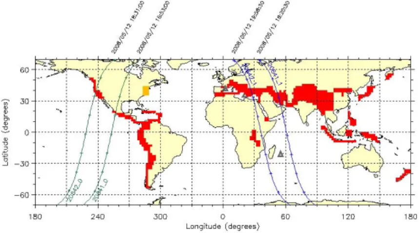
Figure 2.6. Two successive DEMETER orbits: the two dayside
down-going half-orbits are shown in green, the two night-side up-down-going half orbits are shown in blue. The ascending and descending nodes move by ~ 24° westward from one orbit to the next.
22
the remaining intervals of time to get lower time resolution measurements over larger orbit paths which help building parameters reference base-lines and achieve space-weather objectives.
During the six years of DEMETER operational phase, from 2005 to 2010, a number of joint observations were coordinated with the SURA, HAARP and EISCAT high power HF transmitters. The main objectives of these combined experiments fall in two categories, in-situ measurements of plasma and wave disturbances or detection of ELF and VLF wave emissions triggered by the interaction of the HF waves with the ionosphere.
An extensive program was performed with the SURA heating facility. There were ~200 satellite passes over SURA during the 6 years of DEMETER operations. The main goal of this program was to study the formation, structure and characteristics of ducts in the heated ionosphere and their role in ionosphere-magnetosphere coupling and VLF wave propagation. An overview of the results obtained during the DEMETER joint program was given by Frolov et al., [2016] and references therein.
During the DEMETER joint experiments O-mode HF waves were radiated either towards the zenith (antennas at 0° elevation) or at an elevation of 12° South to benefit from the “magnetic zenith effect” [Gurevich, 2007]. In such a configuration, the HF waves are refracted during their travel through the lower ionosphere so that their propagation vector is ~ parallel to the Earth’s magnetic field at their reflection altitude which maximizes the ionospheric disturbances along the corresponding flux tube. The SURA facility was switched on for 10 to 15 minutes before the satellite reached closest distance from the center of the heated magnetic flux tube. This was shown by Vas’kov et al. [1998], Gladevich et al. [2003] and Frolov et al. [2007] to be sufficient for the development of ionospheric disturbances to a stationary level over the full range of altitudes from the pump-wave reflection altitude in the bottom-side F-region to ~ 800 km, about 100-150 km above the DEMETER orbit and at the altitude of the DMSP satellites from which complementary plasma data were obtained in some cases. The heating time was increased to 40 minutes in a few (unsuccessful) cases in 2010 when it was attempted to search for detectable disturbances in the conjugate ionosphere.
Finally, IDP measurements of precipitating energetic electrons provide interesting observations. They demonstrated enhanced electron precipitations in the low energy band (70 < E < 150 keV), which according to the general discussion of IDP observations in Sauvaud et al., [2006] is due to the scattering of radiation belt electrons by a VLF transmitter operating in this longitude zone.
2.2.2 Defense Meteorological Satellite Program (DMSP)
The Defense Meteorological Satellite Program (DMSP) is the longest, more than 50 years, running production satellite program ever. The DMSP spacecraft monitor meteorological, oceanographic, and solar-terrestrial physics for the United States Department of Defense. The last, DMSP 19, satellite was launched on April 3, 2014. Currently, three satellites F16, F17, and F18 are collecting data (F19 is considered lost as of July 2016). Each of the DMSP spacecraft is a
three-23
axis stabilized satellite flying in circular, sun-synchronous polar (inclination 98.7°) orbit at an altitude of ∼840-850 km (see Figure 2.7). The geographic local times of the orbits are either near the 1800-0600 or 2100-0900 meridians. Due to the offset between the geographic and geomagnetic poles DMSP satellites sample a wide range of magnetic local times (MLT) over the course of a day. The ascending nodes of DMSP orbits are on the dusk side of the Earth. Thus, the satellites move toward the northwest in the evening LT sector. Besides meteorological and oceanographic sensors, each satellite carries a sophisticated sensor suite to measure fluxes of auroral particles (SSJ4/5), the densities, temperatures, and drift motions of ionospheric ions and electrons (SSIES), and after 1995 perturbations of the Earth magnetic field (SSM).
Identical SSJ4/5 sensors are mounted on the top sides of DMSP satellites to measure fluxes of precipitating electrons and ions in the energy range between 30 eV and 30 keV. The measurements are made by 4 detectors, one high energy detector and one low energy detector for each of the particle types. The ion detectors have no mass discrimination capabilities. Each detector has 10 logarithmically spaced energy steps. The high energy detectors step from 30 keV to 1 keV and the low energy detectors step from 1 keV to 30 eV. Only particles within an
energy band of approximately 10% of the channel step energy freely pass from aperture to the detector. The particle fluxes are measured within a solid angle of 2° by 5° for the high energy channels and 4° by 5° for the low energy channels centered on local vertical. Each detector has a dwell time of 0.098 sec and a 0.002 sec period between steps to stabilize the voltage. Each detector makes a complete 10 step sequence in 1 second. One 20-point ion and one 20-point electron sequence is returned once per second.
SSIES sensors are mounted on the ram facing surfaces of the satellites. They consist of an ion drift meter to measure the horizontal and vertical cross-track components of plasma drift within the range of ±3000 m/s and a one-bit resolution of 12 m/s for ambient ion densities greater than 5⋅10³cm⁻³, retarding potential analyzer to m easure ion tem peratures, com position, and the in -track component of plasma drift, an ion trap to measure the total ion density, and a spherical Langmuir probe mounted on an 80-cm boom to measure the density and temperature of ambient electrons [Rich and Hairston, 1984]. The drift and density measurements are sampled at 6 and 24 Hz, respectively. It takes 4 seconds to sample temperatures.
SSM sensors are tri-axial fluxgate magnetometers mounted on the bodies of the F12--F14 satellites and since DMSP F15, on 5-m booms to reduce spacecraft-generated electromagnetic contamination. Magnetic field components are sampled at a rate of 12 (Y and Z) and 10 (X) s-1 in a satellite-centered coordinate system. The X axis points in the downward direction. The Y axis points along the spacecraft velocity. The Z axis completes a right-hand coordinate system. Positive Figure 2.7. The artist’s view of a DMSP satellite.
24
Z components generally point in the anti-sunward direction. Data are presented as differences (ΔB) between measured values and those assigned by the IGRF-90 magnetic field model.
In the past decade, various DMSP satellites have been used in conjunction with the SURA, EISCAT, and HAARP heating experiments to measure artificial density ducts and ion outflows in the topside ionosphere [e.g., Frolov et al., 2016; Milikh et al., 2008a; 2010a; Blagoveshchenskaya
et al., 2011].
2.2.3 The Demonstration and Science Experiments (DSX) Satellite
The Air Force Research Laboratory has developed the Demonstration and Science Experiments (DSX) satellite to investigate 1) very-low-frequency electromagnetic wave-particle interactions (WPIx) in medium-earth orbit (MEO) region of space between the Van Allen radiation belts, the “slot” region; 2) space weather effects in the slot region (SWx); and 3) space environmental effects (SFx) on spacecraft components in the slot region [Fennelly, 2009;
Scherbarth et al., 2009]. In addition to the DSX spacecraft, VLF and Particle Mapper (VPM)
nanosatellite will be launched to perform far-field measurements of the in situ transmitter [Gies et
al., 2014]. The DSX mission is planned to be launched in 2018 aboard SpaceX Falcon Heavy for
a nominal one year mission. It will fly in a 6000×12000 km elliptical (42°-inclination) orbit covering the outer region of the inner radiation belt, the slot region, and the inner region of the outer radiation belt in a 5.3 hour period. The planned initial orbit has apogee and perigee near the equator, with an orbit precession period just over one year. Figure 2.8 shows a schematic view of the DSX space flight experiment with the VPM nanosat.
The SFx module [Scherbarth et al., 2009] consists of the NASA Space Environment Testbeds-1 (SET-1) and radiometers and photometers provided by the Air Force Research Laboratory Aerospace Systems Directorate. The objectives of SET-1 are to improve engineering approaches to accommodate and/or mitigate the effect of solar variability on spacecraft design and operations, reduce risk for new technologies infused into future space missions, and provide a standard mechanical, electrical, and thermal interface for a collection of small flight investigations. The SET-1 payload consists of two units, the Correlative Environment Monitor (CEM) and the Central Carrier Assembly (CCA). The carrier provides a single interface for power and data between the
DSX spacecraft and the SET-1 microelectronic investigations (inside the CCA) and CEM.
The WPIx module [Scherbarth et al., 2009] is the one relevant to the topic of this review, so it will be described in more details. The module contains a VLF transmitter, broadband (BBR) and narrowband (NBR) receivers, tri-axial search coil (TASC) and DC vector (VMAG) magnetometers, and loss-cone imager (LCI). The BBR and TASC along with Y and Z linear, orthogonal dipole antennas with two electric components make up the VLF broadband receiver, with the frequency range 0.1 – 50 kHz and the sensitivity 10-16 V2/m2/Hz and 10-11 nT2/Hz. The Figure 2.8. An illustration of the DSX
space flight experiment with the VPM nanosatellite [Fennelly, 2009].
25
receiver was built by Stanford University, NASA/Goddard, Lockheed Martin, and ATK Space Systems. The NBR and Y antenna constitute the VLF narrowband receiver covering the band from 3 kHz to 750 kHz. The LCI consists of a High Sensitivity Telescope (HST) for measuring 100 – 500 keV electrons with 0.1 cm2-str geometric factor within 6.5° loss cone, and a Fixed Sensor Head (FSH) for 50 – 700 keV electrons with 130°×10° pitch angle distribution. The LCI instrument was built by Boston University. Finally, the VMAG instrument is capable of 0 – 8 Hz three axis measurements of magnetic field line measurements at +/- 0.1 nT accuracy. The VMAG was built by the University of California, Los Angeles (UCLA).
The VLF transmitter was built by the University of Massachusetts Lowell (UML), Southwest Research Institute, and ATK. The transmitter will operate in high power at 2 - 50 kHz at the kV level for up to 30 min per orbit occurring near the magnetic equator (|MLAT|<20° or L<3.5) and also will coordinate with conjugate target teams. An additional "sounding" low power mode at 50-750 kHz will also be used for plasma characterization during the mission.
The Z antenna (16 m tip-to-tip) functions as a VLF receive antenna in a cross-dipole configuration with the Y antenna. The TASC and VMAG instruments are placed at opposite tips of the Z antenna (16 m tip-to-tip) to separate them from the rest of the DSX instruments which would interfere with their operation as VMAG and TASC measure the local DC and AC magnetic fields, respectively. The Y antenna (80 m tip-to-tip) functions as a VLF receive and transmit antenna. Their booms are both built by ATK Space Systems.
The Y antenna boom is a truss consisting of Graphite-Epoxy (Gr/Ep) longerons and batten elements with steel diagonals. In order to perform the VLF antenna function, copper wire is run the full length of each truss’s three longerons, attached at every other joint. The Z antenna boom is a similar truss with S-2 glass (fiberglass) material for the longerons and battens instead of the Gr/Ep. Both booms use frangibolt systems to constrain them within canisters through launch. Once on-orbit, the spacecraft powers the frangibolts to heat their Nickel-Titanium (NiTi) collars to the point that they break their bolts and release the tip plates from the canisters. The longerons are continuous elements that are “spring loaded” into the canisters via coiling. Thus, once released, the stored strain energy of each coiled system deploys the structures into their minimally strained, full length trusses. The deployment rate of each truss system is controlled by a lanyard with a geared friction, keeping the trusses from damaging themselves with excessive accelerations and/or sudden decelerations.
The transmitter design is based on NASA’s Imager for Magnetopause-to-Aurora Global Exploration (IMAGE) Radio Plasma Imager (RPI) instrument [Reinisch et al., 2001] that operated at 3 kV and was optimized for > 50 kHz. The DSX design optimizes the transmitter impedance dependent on frequency, antenna length, and diameter. DSX is flying the first ever VLF “dynamic tuning” technology to adjust circuit parameters in real time. The voltages are limited to < 10 kV
26
due to critical component limits. The DSX system is nominally designed for 5 kV with the capability to go to 10 kV at the end of life.
Figure 2.9 shows the functional baseline configuration for the DSX flight experiment. The core is the Evolved Expendable Launch Vehicle (EELV) Secondary Payload Adapter (ESPA) ring, which is used to maximize launch opportunities. The ESPA ring comprises the primary structure for DSX and is upgraded to provide host spacecraft functions (e.g., avionics and power management and distribution) by the addition of components packaged on an avionics module (AM). The DSX payloads (including deployable booms) are mounted on an identical structure, the payload module (PM), attached to the ESPA ring opposite the avionics module. The AM and PM together comprise the DSX Host Spacecraft Bus (HSB). The entire assembly is designed to be stowed within a 4-m diameter EELV fairing.
The VPM nanosat is developed in AFRL/RV to quantify space and terrestrial VLF injection and resulting particle precipitation. The VPM 6U, 10kg spacecraft will be launched from ISS in a circular orbit of 400 km with 51° inclination for 1 year minimum mission. Its payload consists of dual channel VLF receiver, loss cone and trapped electron spectrometers, AC magnetic search coil, deployable E-field antennae, and B-field boom.
2.2.4 RESONANCE Satellite
The international space project RESONANCE [Mogilevsky et al., 2012, Demekhov et al., 2003] is planned with the participation of scientific teams from Russia, Ukraine, Austria, Bulgaria, Germany, Greece, Poland, Slovakia, the USA, Czech Republic, Finland and France and aims to study the resonance interaction of waves and particles in the Earth's inner magnetosphere. A unique part of this project will be a joint experiment with a ground-based facility of RF heating of the ionosphere, which will study of ionospheric physics and test the possibility of controlling some natural powerful processes in the near-Earth plasma.
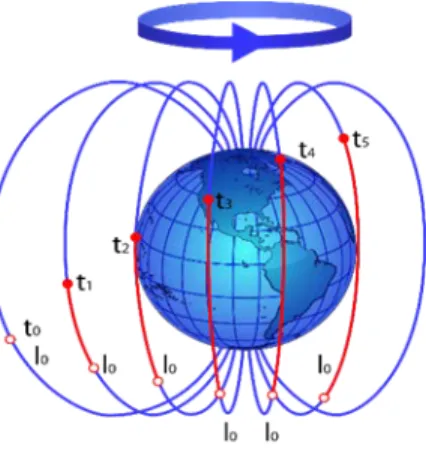
The right choice of the satellite orbits is very important. One of the most interesting options is the possibility of organizing measurements near a specially selected magnetic field line, since particle and energy exchange between the ionosphere and the magnetosphere mainly occur within a tube of force of the Earth’s magnetic field. These processes include in particular: the propagation of whistler-mode and Alfvén waves and the interaction with these waves plays a key role in the electron and ion dynamics in the radiation belts; the precipitation of energetic particles into the ionosphere; the filling of magnetic flux tubes with cold and suprathermal plasma; the motion of energetic particles from the regions of auroral acceleration and regions of magnetic reconnection. To solve these problems requires simultaneous multipoint measurements of plasma parameters and electromagnetic radiation in selected flux tubes of the magnetic field.
One of the main features of the RESONANCE project is the choice of the novel type of a magneto-synchronous orbits proposed and designed for this project that ensure the presence of four satellites in different places of the same magnetic flux tube during a long period of time (relatively to the typical time-scale of magnetospheric processes). The new planned orbital set will consist of two pairs of spacecraft, each pair on its own orbit. The parameters of these orbits are as


![Figure 2.8. An illustration of the DSX space flight experiment with the VPM nanosatellite [Fennelly, 2009]](https://thumb-eu.123doks.com/thumbv2/123doknet/14793455.602511/25.918.557.809.604.847/figure-illustration-dsx-space-flight-experiment-nanosatellite-fennelly.webp)
![Figure 3.2. Schematic representation of the wave spectrum and electron distribution in the developed strong Langmuir turbulence [Shapiro and Shevchenko, 1984]](https://thumb-eu.123doks.com/thumbv2/123doknet/14793455.602511/40.918.496.805.307.511/schematic-representation-spectrum-distribution-developed-langmuir-turbulence-shevchenko.webp)
![Figure 4.2. Variations of the SEE spectral structure in the frequency range f 0 = 4.3 – 9.5 MHz [Frolov et al., 2001]](https://thumb-eu.123doks.com/thumbv2/123doknet/14793455.602511/56.918.113.810.411.763/figure-variations-spectral-structure-frequency-range-mhz-frolov.webp)