HAL Id: hal-00305053
https://hal.archives-ouvertes.fr/hal-00305053
Submitted on 5 Feb 2007
HAL is a multi-disciplinary open access
archive for the deposit and dissemination of
sci-entific research documents, whether they are
pub-lished or not. The documents may come from
teaching and research institutions in France or
abroad, or from public or private research centers.
L’archive ouverte pluridisciplinaire HAL, est
destinée au dépôt et à la diffusion de documents
scientifiques de niveau recherche, publiés ou non,
émanant des établissements d’enseignement et de
recherche français ou étrangers, des laboratoires
publics ou privés.
lumped watershed model identification and evaluation
Y. Tang, P. Reed, Thibaut Wagener, K. van Werkhoven
To cite this version:
Y. Tang, P. Reed, Thibaut Wagener, K. van Werkhoven. Comparing sensitivity analysis methods to
advance lumped watershed model identification and evaluation. Hydrology and Earth System Sciences
Discussions, European Geosciences Union, 2007, 11 (2), pp.793-817. �hal-00305053�
www.hydrol-earth-syst-sci.net/11/793/2007/ © Author(s) 2007. This work is licensed under a Creative Commons License.
Earth System
Sciences
Comparing sensitivity analysis methods to advance lumped
watershed model identification and evaluation
Y. Tang, P. Reed, T. Wagener, and K. van Werkhoven
Department of Civil and Environmental Engineering, The Pennsylvania State University, University Park, Pennsylvania, USA Received: 29 September 2006 – Published in Hydrol. Earth Syst. Sci. Discuss.: 1 November 2006
Revised: 11 January 2007 – Accepted: 30 January 2007 – Published: 5 February 2007
Abstract. This study seeks to identify sensitivity tools that
will advance our understanding of lumped hydrologic mod-els for the purposes of model improvement, calibration effi-ciency and improved measurement schemes. Four sensitivity analysis methods were tested: (1) local analysis using pa-rameter estimation software (PEST), (2) regional sensitivity analysis (RSA), (3) analysis of variance (ANOVA), and (4) Sobol’s method. The methods’ relative efficiencies and ef-fectiveness have been analyzed and compared. These four sensitivity methods were applied to the lumped Sacramento soil moisture accounting model (SAC-SMA) coupled with SNOW-17. Results from this study characterize model sen-sitivities for two medium sized watersheds within the Juni-ata River Basin in Pennsylvania, USA. Comparative results for the 4 sensitivity methods are presented for a 3-year time series with 1 h, 6 h, and 24 h time intervals. The results of this study show that model parameter sensitivities are heav-ily impacted by the choice of analysis method as well as the model time interval. Differences between the two adjacent watersheds also suggest strong influences of local physical characteristics on the sensitivity methods’ results. This study also contributes a comprehensive assessment of the repeata-bility, robustness, efficiency, and ease-of-implementation of the four sensitivity methods. Overall ANOVA and Sobol’s method were shown to be superior to RSA and PEST. Rela-tive to one another, ANOVA has reduced computational re-quirements and Sobol’s method yielded more robust sensi-tivity rankings.
Correspondence to: P. Reed
1 Introduction
In this paper we apply and evaluate the differences between four popular sensitivity analysis methods, selected to repre-sent the variety of methods currently used. The four sensitiv-ity analysis methods include: (1) local analysis using the pa-rameter estimation software (PEST), (2) regional sensitivity analysis (RSA), (3) analysis of variance (ANOVA), and (4) Sobol’s method. The methods are applied to the Sacramento soil moisture accounting model, a medium complexity spa-tially lumped rainfall-runoff model used for river forecasting throughout the USA. The model is implemented in two wa-tersheds in the Susquehanna River Basin in Pennsylvania and run at hourly, six hourly, and daily time steps.
Broadly, models of watershed hydrology are irreplaceable components of water management studies including flood and drought prediction, water resource assessment, climate and land use change impacts, or non-point source pollution analysis (e.g., Singh and Woolhiser, 2002). Hydrologic mod-els are evolving from single purpose tools to complex deci-sion support systems that can perform all (or at least many) of the tasks mentioned above in a single software package. Hydrological models vary in complexity from lumped con-ceptual models to distributed models that include close cou-pling of surface and groundwater flow processes, feedbacks with the atmosphere, transport of water and solutes, and spa-tially explicit representations of system characteristics and states (e.g., Duffy, 1996, 2004; Koren et al., 2004; Panday and Huyakorn, 2004). In integrated assessment applications models may even include socioeconomic components to in-tegrate human behavior (Wagener et al., 2005). In general, hydrologic models are highly non-linear, contain thresholds,
and often have significant parameter interactions. These
properties make it difficult to evaluate how models of hydro-logic systems behave and which parameters control this be-havior during different response modes (e.g., Demaria et al.,
2007). The increasing trend towards more complex mod-els and its potential consequences in terms of computational constraints and obfuscating model impacts on decision mak-ing motivates the need for enhanced model identification and evaluation tools (Beven and Freer, 2001; Vrugt et al., 2003; Saltelli et al., 2004; Wagener and Kollat, 2007).
Hydrologic models play an important role in elucidating the dominant controls on watershed behavior and in this con-text it is important for hydrologists to identify the dominant parameters controlling model behavior. One approach to gain this understanding is through the use of sensitivity anal-ysis, which evaluates the parameter’s impacts on the model response (Hornberger and Spear, 1981; Freer et al., 1996; Wagener et al., 2001; Liang and Guo, 2003; Hall et al., 2005; Pappenberger et al., 2005; Sieber and Uhlenbrook, 2005). Sensitivity analysis results can be used to decide which pa-rameters should be the focus of model calibration efforts, or even as an analysis tool to test if the model behaves accord-ing to underlyaccord-ing assumptions (e.g., Wagener et al., 2003). Ultimately, sensitivity methods should serve as diagnostic tools that help to improve mathematical models and poten-tially help us to identify where gaps in our knowledge are most severe and are most strongly affecting prediction un-certainty. Data gaps are particularly important in the context of guiding field measurement campaigns (Langbein, 1979; Moss, 1979; Wagener and Kollat, 2007; Reed et al., 2006). Section 2 provides a more detailed review of existing sensi-tivity analysis methods and a detailed discussion of the four methods compared in this study.
2 Sensitivity analysis tools and sampling schemes
2.1 Overview
Model sensitivity analysis charaterizes the impact that changes in model inputs have on the model outputs in a strict sense. Model inputs include model parameters, forc-ing, initial conditions, boundary conditions, etc. In this study, we focus on analyzing the sensitivities of model parameters. Sensitivity measures are determined mathematically, statis-tically, or even graphically. There are several prior studies that have broadly reviewed and classified the sensitivity anal-ysis methods that exist (Saltelli et al., 2000, 2004; Helton and Davis, 2003; Oakley and O’Hagan, 2004; Frey and Patil, 2002; Christiaens and Feyen, 2002). Any sensitivity analysis approach can be broken up into to two components (Wagener and Kollat, 2007): (1) a strategy for sampling the model pa-rameter space (and/or state variable space), and (2) a numer-ical or visual measure to quantify the impacts of sampled parameters on the model output of interest. The implemen-tation of these two components varies immensely (e.g., Freer et al., 1996; Frey and Patil, 2002; Hamby, 1994; Patil and Frey, 2004; Pappenberger et al., 2006; Vandeberghe et al., 2007), and guidance is currently lacking to help modelers
decide which approach is best suited to the needs of a par-ticular study. Generally, the approaches can be categorized into two main groups – local methods and global methods (Saltelli et al., 1999; Muleta and Nicklow, 2005).
The nominal range and differential analysis methods are two well known local parameter sensitivity analysis methods (Frey and Patil, 2002; Helton and Davis, 2003). Nominal range sensitivity analysis calculates the percentage change of outputs due to the change of model inputs relative to their baseline (nominal) values. The percentage change is seen as the sensitivity of the corresponding input. Differential anal-ysis utilizes partial derivatives of the model outputs with re-spect to the perturbations of the model input. The deriva-tive values are themselves the metrics of sensitivity. Further analysis can be conducted by approximating the simulation model using Taylor’s series (Helton and Davis, 2003).
The nominal range and differential analysis methods have the advantages of being straightforward to implement while
maintaining modest computational demands. The major
drawback of these methods is their inability to account for parameter interactions, making them prone to underestimat-ing true model sensitivities. Alternatively, global parameter sensitivity analysis methods vary all of a model’s parameters in predefined regions to quantify their importance and poten-tially the importance of parameter interactions.
There are a variety of global sensitivity analysis meth-ods such as regional sensitivity analysis (RSA) (Young, 1978; Hornberger and Spear, 1981), variance based meth-ods (Saltelli et al., 2000), regression based approaches (Spear et al., 1994; Helton and Davis, 2002), and Bayesian sensi-tivity analysis (Oakley and O’Hagan, 2004). Global meth-ods attempt to explore the full parameter space within pre-defined feasible parameter ranges. In this paper, our goal is to test a suite of sensitivity methods and discuss their rela-tive benefits and limitations for advancing lumped watershed model identification and evaluation.
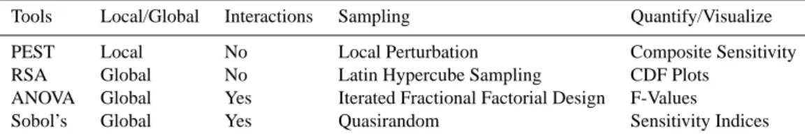
The four sensitivity analysis approaches include one local method termed PEST and three global methods consisting of RSA, analysis of variance (ANOVA), and Sobol’s method. These sensitivity analysis methods were selected for com-parison due to their popularity and their common applica-tion in a variety of scientific domains (Doherty, 2003; Do-herty and Johnston, 2003; Moore and DoDo-herty, 2005; Wa-gener et al., 2003; Lence and Takyi, 1992; Freer et al., 1996; Pappenberger et al., 2005; Mokhtari and Frey, 2005; Sobol’, 1993, 2001; Fieberg and Jenkins, 2005; Hall et al., 2005). The sensitivity analysis methods tested in this study range from local to global and capture a broad range of analy-sis methodologies (differential analyanaly-sis, RSA, and variance-based analysis). The main characteristics of these four meth-ods are summarized in Table 1. In Sect. 2.2, each of these approaches and the associated statistical sampling schemes used in this study are discussed in more detail. In the context of this paper we assume that the selection of an appropriate numerical measure, is satisfied through two chosen
objec-Table 1. Summary of sensitivity analysis tools in the study.
Tools Local/Global Interactions Sampling Quantify/Visualize
PEST Local No Local Perturbation Composite Sensitivity
RSA Global No Latin Hypercube Sampling CDF Plots
ANOVA Global Yes Iterated Fractional Factorial Design F-Values
Sobol’s Global Yes Quasirandom Sensitivity Indices
tive functions based on the root mean square error (RMSE) (see Sect. 5.2). Readers interested in how parameter sensitiv-ity changes with different objective functions can reference the following studies (Wagener et al., 2001; Demaria et al., 2007).
2.2 Sensitivity analysis tools
2.2.1 PEST
PEST, which stands for parameter estimation, is a model independent nonlinear parameter estimation tool (Doherty, 2003; Doherty and Johnston, 2003; Doherty, 2004; Moore
and Doherty, 2005). PEST was developed to facilitate
data interpretation, model calibration and predictive analy-sis. Like many other parameter estimation or model calibra-tion tools, PEST aims to match the model simulacalibra-tion with an observed set of data by minimizing the weighted sum of squared differences between the two. The optimization prob-lem is iteratively solved by linearizing the relationship be-tween a model’s output and its parameters. The linearization is conducted using a Taylor series expansion where the par-tial derivatives of each model output with respect to every parameter must be calculated at every iteration. For each it-eration, the solution of the linearized problem is the current optimal set of parameters. The current optimal set is then compared to that of the previous time step to determine when to terminate the optimization process. During the lineariza-tion step, the forward difference or central difference oper-ators can be used for calculating the derivatives. Parameter ranges, initial parameter values, and parameter increments must be provided by the user. The parameter vector is up-dated at each step using the Gauss-Marquardt-Levenberg al-gorithm (Marquardt, 1963; Levenberg, 1944). The deriva-tives of the model outputs with respect to its parameters are calculated and provide a measure of the parameter sensitivi-ties at each iteration. The “composite sensitivity” is provided by PEST as a byproduct of the parameter estimation results. The composite sensitivity of parameter i is defined as:
si = (JtQJ)1/2ii /m (1)
where J is the Jacobean matrix and Q is the cofactor ma-trix which in most cases is a diagonal mama-trix whose elements are composed of squared weights for model outputs. If the
model outputs are equally weighted, Q is equal to the iden-tity matrix. The number of outputs, m, is the number of data
records in the time series in this study. Thus siis the
normal-ized magnitude of the Jacobean matrix column with respect to parameter i. As expected for a local sensitivity analysis method, Eq. (1) is a univariate analysis of parameter impacts on model outputs (i.e., no parameter interactions are consid-ered).
2.2.2 Regional sensitivity analysis using Latin hypercube
sampling
RSA (Young, 1978; Hornberger and Spear, 1981) is also called generalized sensitivity analysis (GSA) (Freer et al., 1996) and has been widely used in hydrology (e.g., Lence and Takyi, 1992; Spear et al., 1994; Freer et al., 1996; Pappenberger et al., 2005; Sieber and Uhlenbrook, 2005;
Ratto et al., 2006). Monte Carlo sampling and
“behav-ioral/nonbehavioral” partitioning are the two major compo-nents of this method. Monte Carlo sampling is used to gen-erate n parameter sets in the feasible parameter space de-fined using a multi-variate uniform distribution. After model evaluations using these parameters, the sets of parameters are decomposed into two separate groups (behavioral/good and nonbehavioral/bad) according to the model’s performance or behavior. RSA identifies the difference between the un-derlying distributions of the behavioral and nonbehavioral groups. Either graphical methods (e.g., marginal cumula-tive distribution function plots) or statistical methods such as Kolmogorov-Smirnov (KS) testing (Kottegoda and Rosso, 1997) are then used to characterize if a parameter signifi-cantly impacts behavioral results.
Freer et al. (1996) extended the original RSA by breaking the behavioral parameter sets into ten equally sized groups. (Wagener et al., 2001) modified this approach further by in-cluding all parameter sets and avoiding the need to specify behavioral and non-behavioral sets. Instead, the population is divided into ten bins of equal size based on a sorted model performance measure (Wagener and Kollat, 2007). Conclu-sions about parameter sensitivities are made qualitatively by examining differences in the marginal cumulative distribu-tions of a parameter within each of the ten groups. Ten lines in the RSA plot represent the cumulative distributions of a parameter with respect to ten sampled sub-ranges. If the lines are clustered, the parameter is not sensitive to a
spe-cific model performance measure. Conversely, the degree of dispersion of the lines is a visual measure of a model’s sen-sitivity to an input parameter. Wagener and Kollat (2007) implemented the original idea of Freer et al. (1996) visually using the Monte Carlo analysis toolbox (MCAT) (Wagener et al., 2001, 2003, 2004) where the marginal cumulative dis-tributions of the ten groups are plotted as the likelihood value versus the parameter values.
In this study, Latin hypercube sampling (LHS) was used to sample the feasible parameter space for testing RSA based on the recommendations and findings of prior studies (e.g., Os-idele and Beck, 2001; Sieber and Uhlenbrook, 2005). LHS integrates random sampling and stratified sampling (Mckay et al., 1979; Helton and Davis, 2003) to make sure that all portions of the parameter space are considered. The method divides the parameters’ ranges into n disjoint intervals with equal probability 1/n from which one value is sampled ran-domly in each interval. LHS is generally recommended for sparse sampling of the parameter space and the parameter interactions are neglected as noted by William et al. (1999). More details about LHS are available in the following papers (Mckay et al., 1979; Helton and Davis, 2003; William et al., 1999).
2.2.3 Analysis of variance using iterated fractional factorial
design sampling
Assuming model response (e.g., RMSE of streamflow in this study) is normally distributed, the role of ANOVA is to quan-tify the differences of the mean model responses that result from samples of each parameter. In ANOVA, parameters are “grouped” into particular ranges of parameter values repre-senting intervals with equal parameter value width, contrast-ing to RSA in which parameter sets are “grouped” based on model response measures such as the RMSE of stream-flow predictions used in this study. According to ANOVA terminology, a parameter is called a “factor” and a parame-ter group is parame-termed a “level” of the factor. ANOVA essen-tially partitions the model output or response into the overall mean, main factor effects, factor interactions, and an error term (Neter et al., 1996; Mokhtari and Frey, 2005). Theo-retically, ANOVA can capture a range from the first order (main effects from single parameters) to the total order of ef-fects (i.e., all parameter impacts including all interactions). However, it is not feasible to calculate all of the effects for a complex model in practice due to computational limita-tions. Fortunately, prior studies have shown that second or-der interactions are usually sufficient for capturing a model’s output variance (Box et al., 1978; Henderson-Sellers et al., 1993; Liang and Guo, 2003). Therefore, our analysis focuses on first order and second order effects within the ANOVA model. The model response variable Y is decomposed into main and second order effects of two factors according to
2-way ANOVA model:
Yij k = µ + αi+ βj+ (α × β)ij+ εij k (2)
where i and j indicate the levels of factors A and B
respec-tively, αi is the main effect of ith level of A, βj is the main
effect of j th level of B, (α × β)ij represents the interaction
of A and B. The error term, εij k, reflects the effects that are
not explained by the main effects and interactions of the two factors. Variable k represents the kth value of Y .
The F -test is used to evaluate the statistical significance of differences in the mean responses among the levels of each parameter or parameter interaction. The F values are cal-culated for all parameters and parameter interactions. The higher the F values are, the more significant the differences are and therefore the more sensitive the parameter or param-eter interaction is. Detailed presentation of the ANOVA cal-culation table for main effects and second order effects can be found in other studies (Neter et al., 1996; Mokhtari and Frey, 2005). In addition to the F-test, the coefficient of
de-termination (r2) quantifies how the ANOVA model shown in
Eq. (2) captures the total variation of model responses with the inclusion of the second order parameter interactions. In cases where parameter interactions are important the coeffi-cient of determination should improve (or increase) with the
addition of the interaction term (α × β)ijfrom Eq. (2).
When applying the ANOVA method the statistical sam-pling scheme used to quantify the model response is a key de-terminant of the method’s computational feasibility and ac-curacy. If one parameter or parameter interaction is analyzed at a time in succession, the total number of model runs will be excessively large and most hydrologic applications would be computationally intractable. In this study, the iterated frac-tional factorial design (IFFD) sampling scheme (Andres and Wayne, 1993; Andres, 1997; Saltelli et al., 1995) was used to limit the computational burden posed by ANOVA while seeking high quality results.
IFFD works well when first and second order parameter effects dominate (Andres, 1997). Using IFFD in ANOVA al-lows users to neglect higher order interactions not included in the model (Liang and Guo, 2003; Andres, 1997) while gen-erating highly repeatable results (Saltelli et al., 1995). Con-sequently, the number of model runs required can be reduced substantially. IFFD as implemented in this study samples the parameters at three different levels: low, middle, and high. The parameter levels are defined as equally spaced inter-vals within the predefined parameter ranges. Using a small number of factor levels enables the sampling scheme to at-tain statistically significant results efficiently and accurately (Mokhtari and Frey, 2005; Andres, 1997). IFFD extends the basic orthogonal fractional factorial design (FFD) by con-ducting multiple iterations. The basic operations in IFFD include orthogonalization, folding, replication and random sampling (Andres and Wayne, 1993; Andres, 1997; Saltelli et al., 1995). The orthogonalized design guarantees equal
frequency for two parameter combinations but also differen-tiates the main effects from two-way interactions. A detailed presentation of IFFD is beyond the scope of this paper. Read-ers interested in detailed descriptions of IFFD are referred to the following papers (Andres and Wayne, 1993; Andres, 1997; Saltelli et al., 1995).
2.2.4 Sobol’s method using quasi-random sequence
sam-pling
In Sobol’s method (Sobol’, 1993), the variance of the model output is decomposed into components that result from in-dividual parameters as well as parameter interactions. Con-ventionally, the direct model output is replaced by a model performance measure such as RMSE as used in this study. The sensitivity of each parameter or parameter interaction is then assessed based on its contribution (measured as a per-centage) to the total variance computed using a distribution of model responses. Assuming the parameters are indepen-dent, the Sobol’s variance decomposition is:
D(y) =X i Di + X i<j Dij + X i<j <k Dij k+ D12···m (3)
where Di is the measure of the sensitivity to model output y
due to the ith component of the input parameter vector
de-noted as 2, Dij is the portion of output variance that results
due to the interaction of parameter θiand θj. The variable m
defines the total number of parameters. The variance decom-position shown in Eq. (3) can be used to define the sensitivity indices of different orders as:
first order Si = Di D (4) second order Sij = Dij D (5) total ST i= 1 − D∼i D (6)
where Si denotes the sensitivity that results from the main
ef-fect of parameter θi. The second order sensitivity index, Sij,
defines the sensitivity that results from the interaction of
pa-rameters θi and θj. The average variance, D∼i, results from
all of the parameters except for θi. The total order sensitivity,
ST i, represents the main effect of θias well as its interactions
up to mt horder of analysis. A parameter which has a small
first order index but large total sensitivity index primarily im-pacts the model output through parameter interactions.
The variances in Eq. (3) can be evaluated using approxi-mate Monte Carlo numerical integrations. The Monte Carlo
approximations for D, Di, Dij, and D∼i are defined as
pre-sented in the following prior studies (Sobol’, 1993, 2001; Hall et al., 2005): b f0= 1 n n X s=1 f (2s) (7) b D = n1 n X s=1 f2(2s) − bf0 2 (8) c Di = 1 n n X s=1
f (2(a)s )f (2(b)(∼i)s, 2(a)is ) − bf0 2 (9) d Dij c = 1 n n X s=1
f (2(a)s )f (2(b)(∼i,∼j )s, 2(a)(i,j )s) − bf0 2 (10) d Dij = dDij c − cDi− cDj (11) d D∼i = 1 n n X s=1
f (2(a)s )f (2(a)(∼i)s, 2(b)is ) − bf0 2
(12)
where f is the model response, term n is the sample size,
2s denotes the sampled individual in the scaled unit
hyper-cube, and (a) and (b) are two different samples. All of the parameters take their values from sample (a) are represented
by 2(a)s . The variables 2(a)is and 2
(b)
is denote that parameter
θi uses the sampled values in sample (a) and (b),
respec-tively. The symbols 2(b)(∼i)s and 2(b)(∼i)s represent cases when
all of the parameters except for θi use the sampled values in
sample (a) and (b), respectively. The symbol 2(a)(i,j )s
rep-resents parameters θi and θj with sampled values in sample
(a). Finally, 2(a)
(∼i,∼j )s represents the case when all of the
parameters except for θi and θj utilize sampled values from
sample (b).
The original Sobol’s method required n×(2m+1) model runs to calculate all the first order and the total order sensitiv-ity indices. An enhancement of the method made by Saltelli (2002) provides the first, second and total order sensitivity indices using n×(2m+2) model runs. In this study, we im-plemented this modified version of Sobol’s methodology to compute the first order, second order and total order indices. The convergence of the Monte Carlo integrations used in Sobol’s method is heavily affected by the sampling scheme selected. The error term in the Monte Carlo integration
de-creases as a function of 1/√n given uniform, random
sam-ples at n points in the m-dimensional space. However, in this study we elected to use Sobol’s quasi-random sequence (Sobol’, 1967; Sobol, 1994) to increase the convergence rate to nearly 1/n. The quasi-random sequence samples points more uniformly along the Cartesian grids than uncorrelated random sampling. Details about Sobol’s quasi-random se-quence can be found in the following studies (Sobol’, 1967; Sobol, 1994; Bratley and Fox, 1988; William et al., 1999).
3 Overview of the lumped hydrologic models
The SNOW-17 (Anderson, 1973) and the Sacramento soil moisture accounting (SAC-SMA) models (Burnash, 1995) are popular and the United States National Weather Service (US NWS) uses them for river forecasting (Moreda et al., 2006; Koren et al., 2004; Smith et al., 2004; Reed et al., 2004). In this study, lumped versions of these models have
Precipitation Air Temperature
Snow Accumulation SCF, PXTEMP
Areal Extent of snow cover SI, Depletion Curve Surface Melt
MFMAX, MFMIN, UADJ, MBASE
Heat Storage & Water Retention NMF, TIPM, PLWHC
Ground Melt DAYGM
Fig. 1. Major SNOW-17 processes and their corresponding
param-eters. MBASE-Base temperature for snowmelt computations dur-ing nonrain periods (degc). NMF-Maximum negative melt factor (mme/degc/6hr). TIPM-Antecedent temperature index parameter. PLWHC-Percent (decimal) liquid-water holding capacity. DAYGM – Constant amount of melt which occurs at the snow-soil interface whenever snow is present (mm). The full description of other pa-rameter names can be found in Sect. 3.1 and in Table 2. Shaded boxes represent the states or processes.
been coupled where SAC-SMA uses SNOW-17’s outputs as forcing. Sections 3.1 and 3.2 provide brief overviews of both models.
3.1 SNOW-17
SNOW-17 (Anderson, 1973) is a conceptual model that sim-ulates the energy balance of a snowpack using a tempera-ture index method. Air temperatempera-ture and precipitation are the model inputs. The states and processes include snow melt, snow cover accumulation, surface energy exchange during non-melt periods, snow cover heat storage, areal extent of snow cover, retention and transmission of liquid water, and heat exchange at the snow-soil interface. Snow melt, snow cover accumulation, and areal extent are the three most influ-ential components in the model.
Snow melt is calculated separately for rain-on-snow pe-riods and non-rain pepe-riods. The snow melt during rain-on-snow periods is computed based on energy and mass bal-ance equations with average wind function (UADJ) as the only parameter. In contrast, snow melt during non-rain pe-riods is calculated empirically. The maximum melt factor (MFMAX) and the minimum melt factor (MFMIN) con-trol this calculation. When calculating the accumulation of snow cover, the form of precipitation is simply determined by a threshold temperature (PXTEMP). The snowfall correc-tion factor (SCF) adjusts gage precipitacorrec-tion estimates for bi-ases during snowfall. To determine the areal extent of snow cover, a pre-defined depletion curve relates the areal extent to areal water equivalent based on the historical maximum
wa-ter equivalent and the wawa-ter equivalent above which 100% of snow cover exists. Process calculations are described in more detail in Anderson (1973). The main processes and corre-sponding twelve model parameters in SNOW-17 are shown in Fig. 1. Based on the prior work of Anderson (2002), we have focused our sensitivity analysis on five of SNOW-17’s parameters (excluding the areal depletion curve ). These five parameters and their allowable ranges (Anderson, 2002) are summarized in Table 2.
3.2 Sacramento soil moisture accounting model
The SAC-SMA model (Burnash, 1995) is a sixteen parame-ter lumped conceptual waparame-tershed model used for operational river forecasting by the US NWS. It represents the soil col-umn by an upper and lower zone of multiple storages. The upper zone is divided into free water and tension water stor-ages. The tension water spills into the free water storage only when the tension water storage (UZTWM) is filled. The free water in the upper zone can then move laterally as interflow or move vertically down to the lower zone as percolation. Ca-pacities of the two storages are model parameters (UZFWM and UZTWM), while the volume of water in each at any time step are model states. Similar to the upper zone, the lower zone also has tension water and free water storages. The free water in the lower zone is further partitioned into two types: primary and supplemental free water storages, both of which can contribute to base-flow but drain independently at differ-ent speeds following Darcy’s law. The maximum storages for these different types of lower zone free water are the lower zone maximum tension water (LZTWM), the primary free water (LZFPM), and the supplemental free water (LZFSM). SAC-SMA’s processes and parameters are illustrated in more detail in Fig. 2. It is indicated in the figure that there are four principal forms of runoff generated by SAC-SMA: 1) direct runoff on the impervious area, 2) surface runoff when the upper zone free water storage is filled and the precipita-tion intensity is greater than percolaprecipita-tion and interflow rate, 3) the lateral interflow from upper zone free water storage, and 4) primary baseflow. The direct runoff is composed of the impervious runoff over the permanent impervious area and the direct runoff on the temporal impervious area. The permanent impervious area, represented by parameter PC-TIM (percent of impervious area), represents constant im-pervious areas such as pavements. The temporal imim-pervious area, represented by parameter ADIMP (additional impervi-ous area), includes the filling of small reservoirs, marshes, and temporal seepage outflow areas which become impervi-ous when the upper zone tension water is filled. Prior work (Peck, 1976) has shown that thirteen out of sixteen parame-ters control model performance and must be calibrated. Fea-sible ranges of these thirteen parameters are presented by Boyle et al. (2000) and also used in the calibration studies of Tang et al. (2006, 2007) and Vrugt et al. (2003) (see Ta-ble 2). As shown in TaTa-ble 2, the maximum allowaTa-ble value of
Table 2. Summary of SNOW-17 and SAC-SMA parameters.
Model Parameters Unit Description Allowable Range
SCF Gage catch deficiency adjustment factor 1.0–1.3
MFMAX mm/◦C/6 h Maximum melt factor during non-rain periods 0.5–1.2 SNOW-17 MFMIN mm/◦C/6 h Minimum melt factor during non-rain periods 0.1–0.6 UADJ mm/mb/6 h Average wind function during rain-on-snow periods 0.02–0.2 SI mm Mean water-equivalent above which 100% cover exists 10–120 UZTWM mm Upper zone tension water maximum storage 1.0–150.0 UZFWM mm Upper zone free water maximum storage 1.0–150.0 UZK day−1 Upper zone free water lateral depletion rate 0.1–0.5 PCTIM Impervious fraction of the watershed area 0.0–0.1
ADIMP Additional impervious area 0.0–0.4
ZPERC Maximum percolation rate 1.0–250.0
SAC-SMA REXP Exponent of the percolation equation 0.0–5.0
LZTWM mm Lower zone tension water maximum storage 1.0–500.0 LZFSM mm Lower zone free water supplemental maximum storage 1.0–1000.0 LZFPM mm Lower zone free water primary maximum storage 1.0–1000.0 LZSK day−1 Lower zone supplemental free water depletion rate 0.01–0.25 LZPK day−1 Lower zone primary free water depletion rate 0.0001-0.025 PFREE Fraction of water percolating from upper zone directly to lower
zone free water storage
0.0–0.6
Pervious Area, RIVA PCTIM, ADIMP
ET Precipitation
UZTWM UZFWM
ZPERC, REXP, PFREE
LZTWM LZFPM LZFSM RSERV LZPK LZSK SIDE Direct Runoff Channel Flow Surface Runoff UZK Subsurface Discharge Surface Upper Zone Lower Zone ET
Fig. 2. Major SAC-SMA processes and their corresponding parameters. RIVA-Riparian vegetation area. SIDE-Ratio of deep recharge to
channel base flow. RSERV-Fraction lower zone free water not transferable to tension water. The full description of other parameter names can be found in the Table 2. The parameters in the shaded boxes pertain to storages or states.
ADIMP specified by the author is 0.4 indicating that 40% of the watershed area is the additional impervious area, which can lead to large direct runoff under wet conditions.
4 Case study
4.1 Juniata watershed description
The Juniata Watershed, part of the Susquehanna River Basin,
covers an area of 8800 km2 in the ridge and valley region
of the Appalachian Mountains of south central
Pennsylva-nia. The watershed is within the US NWS mid-Atlantic
river forecast center (MARFC) area of forecast responsibil-ity. The primary aquifer formations are composed of sedi-mentary and carbonate rocks that are presented in alternating layers of sandstone, shale, and limestone. Approximately, 67 percent of the watershed is forested, 23 percent is agricul-tural, 7 percent is developed area, and the rest is mine lands, water, or miscellaneous. There are 11 major sub-watersheds (see Fig. 3), among which, RTBP1, LWSP1, MPLP1, and NPTP1 have heavily controlled flows from reservoirs. Our preliminary analysis of the watershed focused on 7 headwa-ter sub-waheadwa-tersheds where flows are not managed. Figure 4 illustrates our preliminary analysis of the hydrologic
condi-SXTP1 WLBP1 SPKP1 HUNP1 MPLP1 REEP1 NPTP1 PORP1 SLYP1 RTBP1 LWSP1 0 15 30 60Kilometers
±
Fig. 3. Sub-watersheds in the Juniata river basin.
tions within the seven sub-watersheds by plotting their flow duration curves as well as monthly averages for streamflow, potential evaporation, and precipitation. Figure 4 shows that the SPKP1 (Spruce Creek) and SXTP1 (Saxton) watersheds have distinctly different flow regimes. In the remainder of our study, we have evaluated the model sensitivities within these two watersheds using the four sensitivity analysis tools introduced in Sect. 2. As will be discussed in more detail in Sect. 5, our analysis evaluates model sensitivities for differ-ent temporal and spatial scales (i.e., SPKP1 and SXTP1 have
drainage areas of 570 and 1960 km2, respectively).
4.2 Data set
The SAC-SMA/SNOW-17 lumped model used required in-put forcing data consisting of precipitation, potential evap-otranspiration (PE), and air temperature. The precipitation data are next generation radar (NEXRAD) multisensor pre-cipitation estimator data from the US NWS. Hourly data for precipitation and air temperature were available from 1 Jan-uary 2001 to 31 December 2003. The observed streamflow in the same period was obtained from United States Geolog-ical Survey (USGS) gauge stations located at the outlets of the SPKP1 and SXTP1 watersheds.
5 Computational experiment
5.1 Model setup and parameterizations
In this study, we used a Linux computing cluster with 133 computer nodes composed of dual or quad AMD Opteron processors and 64 GB of RAM. Two month warmup periods (1 January to 28 Feburary 2001) were used to reduce the in-fluence of initial conditions. Model performance was
evalu-ated using three different time intervals (1 h, 6 h, 24 h) to test how parameter sensitivities change due to different predic-tion time scales. The a priori parameter settings used for the SNOW-17 and SAC-SMA models where based on the rec-ommendations of the Mid-Atlantic River Forecasting Center of the US NWS.
The primary algorithmic parameters for PEST were set based on the recommendations of Doherty (2004). The initial Marquardt lambda and its adjust factor were set to be 5 and 2 respectively. When calculating the derivatives, the param-eters were incremented by a fraction of the current parame-ters’ values subject to the absolute increment lower bounds. The fraction is 0.01 and the lower bounds vary from param-eter to paramparam-eter based on their magnitudes. The paramparam-eter estimation process terminates if one of the following condi-tions is satisfied: 1) the number of iteracondi-tions exceeds 30; 2) the relative difference between the objective value of the cur-rent iteration and the minimum objective value achieved to date is less than 0.01 for 3 successive iterations; 3) the al-gorithm fails to lower the objective value over 3 successive iterations; 4) the magnitude of the maximum relative param-eter change between optimization iterations is less than 0.01 over 3 successive iterations.
Statistical sample sizes are key parameters for RSA, ANOVA, and Sobol’s method. In this study, the sample sizes were configured based on both literature recommendations and experiments by observing the convergence and repro-ducibility of the sensitivity analysis results. Sieber and Uh-lenbrook (2005) used a sample size of 10 times the number of perturbed parameters while doing sensitivity analysis on a distributed catchment model using LHS. However, the exper-imental analysis showed this is far from enough for our study. Examining statistical convergence as a function of increasing sample size, we determined a size of 10 000 was sufficient for LHS in RSA. For the ANOVA method, typically the F values increase for the sensitive parameters with increases in sample size (Mokhtari and Frey, 2005). Our analysis of convergence for the ANOVA method’s F-values and parameter sensitivity rankings showed that a sample size of 1,000 was sufficient when using IFFD sampling. For Sobol’s quasi-random se-quence Sobol’ (1967) states that additional uniformity can be obtained if the sample size is increased according to the
function n=2k, where k is an integer. Building on this
rec-ommendation, our analysis showed that Sobol’s sensitivity indices converged and were reproducible using a sample size
8,192 (213).
5.2 Objective functions
Two different model performance objective functions were used to screen the sensitivity of SAC-SMA and SNOW17 for high streamflow and low streamflow. The first objective was the non-transformed root mean square error (RMSE) ob-jective, which is largely dominated by peak flow prediction errors due to the use of squared residuals. The second
ob-0 10 20 30 40 50 60 70 80 90 100 10−4 10−3 10−2 10−1 100 101 102 103
Percentage of time flow exceeded (%)
Daily streamflow (mm/d) NPTP1 PORP1 REEP1 SLYP1 SPKP1 SXTP1 WLBP1 10−5 1 2 3 4 5 6 7 8 9 10 11 12 0 30 60 90 120 Month Average streamflow (mm) Average Precipitation (mm ) 0 30 60 90 120 0 20 40 60 80 100 120 140 Average PE (mm)
Monthly Average Data Flow Duration Curve
1 1.1 1.2 1.3 1.4 1.5 0 0.2 0.4 0.6 0.8 1 P/PE Q/P NPTP1 PORP1 REEP1 SLYP1 SPKP1 SXTP1 WLBP1
Fig. 4. Hydrologic conditions of headwater sub-watersheds in the Juniata River basin.
jective was formulated using a Box-Cox transformation of
the hydrograph (z=[(y+1)λ−1]/λ where λ=0.3) as
recom-mended by Misirli et al. (2003) to reduce the impacts of het-eroscedasticity in the RMSE calculations (also increasing the influence of low flow periods).
5.3 Bootstrap confidence intervals
For ANOVA and Sobol’s method, the F values and sen-sitivity indices can have a high degree of uncertainty due to random number generation effects (Archer et al., 1997; Fieberg and Jenkins, 2005). In this study, we used the boot-strap method (Efron and Tibshirani, 1993) to provide confi-dence intervals for the parameter sensitivity rankings for both ANOVA and Sobol’s method. Essentially, the samples gen-erated by IFFD or Sobol’s sequence were resampled N times when calculating the F values or sensitivity indices for each parameter, resulting in a distribution of the F values or in-dices. The moment method (Archer et al., 1997) was adopted for acquiring the bootstrap confidence intervals (BCIs) for this paper. The moment method is based on large sample theory and requires a sufficiently large resampling dimension to yield symmetric 95% confidence intervals. In this study, the resample dimension N was set to 2000 based on prior literature discussions as well as computational experiments that confirmed a symmetric distribution for standard errors. Readers interested in detailed descriptions of the
bootstrap-ping method used in this paper can reference the following sources (Archer et al., 1997; Efron and Tibshirani, 1993).
5.4 Evaluation of sensitivity analysis results
As argued by Andres (1997), good sensitivity analysis tools should generate repeatable results using a different sample set to evaluate model sensitivities. The effectiveness of a sensitivity analysis method refers to its ability to correctly identify the influential parameters controlling a model’s per-formance. Building on Andres (1997), we have tested the ef-fectiveness of each of the sensitivity methods using an inde-pendent LHS-based random draw of 1000 parameter groups for the 18 parameters analyzed in this study.
The independent sample and the sensitivity classifications from each of the sensitivity analysis methods were combined to develop three parameter sets. Set 1 consists of the full ran-domly generated independent sample set of 1000 parameter groups. In Set 2, the parameters classified as highly sensi-tive or sensisensi-tive are set to a priori values while the remaining insensitive parameters are allowed to vary randomly. Lastly, in Set 3 the parameters classified as being highly sensitive or sensitive vary randomly and the insensitive parameters are set to a priori values.
Varying parameters that are correctly classified as insensi-tive in Set 2 should theoretically yield a zero correlation with the full random sample of Set 1 (i.e., plot as a horizontal
Table 3. PEST sensitivities based on the RMSE measure. Dark
gray shading designates highly sensitive parameters defined using a threshold value of 1.0. Light gray designates sensitive parameters defined using a threshold value of 0.01. White cells in the table designate insensitive parameters.
Model Parameter SPKP1 SXTP1 1h 6h 24h 1h 6h 24h SCF 0.04 0.18 0.31 0.11 0.35 0.55 MFMAX 0 0.07 0.01 0 0.05 0.11 SNOW-17 MFMIN 0.03 0.16 0.42 0.03 0.18 0.64 UADJ 0.01 0.10 0.50 0.02 0.13 0.35 SI 0 0 0 0 0 0 UZTWM 0 0 0.01 0 0 0.01 UZFWM 0 0 0 0 0 0 UZK 0.03 0.07 0.16 0.55 1.15 2.26 PCTIM 0.30 0.57 1.03 0.69 1.65 3.05 ADIMP 0.17 0.34 0.60 0.36 0.79 1.71 ZPERC 0 0 0 0.01 0.01 0.02 SAC-SMA REXP 0.01 0.01 0.07 0 0.01 0.04 LZTWM 0 0 0 0 0 0 LZFSM 0 0 0 0 0 0 LZFPM 0 0 0 0 0 0 LZSK 0.14 0.20 0.58 1.30 5.04 10.06 LZPK 1.59 1.11 5.54 0.21 0.14 32.61 PFREE 0.01 0.01 0.08 0.03 0.10 0.03
line). If some parameters are incorrectly classified as insen-sitive then the scatter plots show deviations from a horizon-tal line and increased correlation coefficients. Conversely, if the correct subset of sensitive parameters is sampled ran-domly (i.e., Set 3) then they should be sufficient to capture model output from the random samples of the full parameter set in Set 1 yielding a linear trend with an ideal correlation coefficient of 1. We extended the evaluation methodology of Andres (1997) by calculating the corresponding correlation coefficients instead of using scatter plots.
6 Results
Sections 6.1–6.4 present the results attained for each of the four sensitivity analysis methods tested in this study. Results are presented for the SPKP1 and SXTP1 watersheds at 1 h, 6 h, and 24 h timescales. Section 6.5 then provides a detailed analysis of how the results from each sensitivity method compare in terms of their selection of highly sensitive, sen-sitive, and insensitive parameters for the SAC-SMA/SNOW-17 lumped model. Additionally, Sect. 6.5 builds on the work of Andres (1997) to evaluate the relative effectiveness of the methods in identifying the key input parameters controlling model performance. Detailed conclusions on how individual watershed properties impact model performance are beyond the scope of this paper.
Before discussing the sensitivity results in detail, it is worth noting that there are several ways that sensitivity
anal-Table 4. PEST sensitivities based on the TRMSE measure. Dark
gray shading designates highly sensitive parameters defined using a threshold value of 0.1. Light gray designates sensitive parameters defined using a threshold value of 0.001. White cells in the table designate insensitive parameters.
Model Parameter SPKP1 SXTP1 1h 6h 24h 1h 6h 24h SCF 0.004 0.014 0.022 0.007 0.020 0.033 MFMAX 0.001 0.006 0.001 0 0.002 0.001 SNOW-17 MFMIN 0.002 0.008 0.019 0.008 0.016 0.025 UADJ 0.001 0.005 0.009 0.001 0.007 0.010 SI 0 0 0 0 0 0 UZTWM 0 0 0.001 0 0 0.001 UZFWM 0 0 0 0 0 0 UZK 0.007 0.008 0.047 0.061 0.095 0.134 PCTIM 0.041 0.080 0.159 0.100 0.227 0.419 ADIMP 0.020 0.038 0.078 0.020 0.045 0.121 ZPERC 0 0 0.003 0.001 0.002 0 SAC-SMA REXP 0.001 0.001 0.001 0 0.001 0.005 LZTWM 0 0 0.001 0 0 0.001 LZFSM 0 0 0 0 0 0 LZFPM 0 0 0 0 0 0 LZSK 0.014 0.024 0.075 0.059 0.353 0.006 LZPK 0.258 0.449 0.713 0.332 5.024 2.513 PFREE 0.004 0.007 0.016 0.005 0.006 0.009
ysis methods can be evaluated and used in the context of
watershed model identification and evaluation. The
cur-rent study builds on the optimization research of Tang et al. (2006) by focusing on how well PEST, RSA, ANOVA, and Sobol’s method can identify the set of model input param-eters that control model performance. Successful screening of the relative importance of input parameters and their in-teractions can help to limit the dimensionality of calibration search problems and serve to enhance the efficiency of un-certainty analysis. Recall from Sect. 5 that the model perfor-mance objectives used in this study evaluate the influence of high streamflow conditions via the RMSE measure and low streamflow conditions via the Box-Cox transformed RMSE (TRMSE). Small values of these measures implies that the SAC-SMA/SNOW-17 streamflow projections closely match observations in the simulated period.
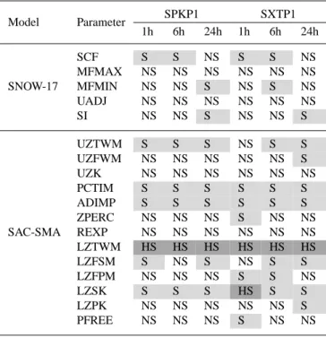
6.1 Sensitivity results for PEST
In the case of PEST, sensitivities are computed using the Jacobean derivative-based composite measures defined in Eq. (1). The method is termed local because the compos-ite derivatives are evaluated at a single point in the param-eter space deemed locally optimal by the Gauss-Marquardt-Levenberg algorithm. Tables 3 and 4 provide the sensitivi-ties computed by PEST for the RMSE and TRMSE objec-tives, respectively. In the tables, highly sensitive parameters are designated with dark grey shading, sensitive parameters have light grey shading, and insensitive parameters are not shaded. The SNOW-17 and SAC-SMA parameters are listed
Table 5. RSA sensitivities based on the RMSE measure. Dark
gray shading designates highly sensitive (HS) parameters. Light gray designates sensitive (S) parameters. White cells in the table designate parameters that are not sensitive (NS).
Model Parameter SPKP1 SXTP1 1h 6h 24h 1h 6h 24h SCF S S NS S S NS MFMAX NS NS NS NS NS NS SNOW-17 MFMIN NS NS S NS S NS UADJ NS NS NS NS NS NS SI NS NS S NS NS S UZTWM S S S NS S S UZFWM NS NS NS NS NS S UZK NS NS NS NS NS NS PCTIM S S S S S S ADIMP S S S S S S ZPERC NS NS NS S NS NS SAC-SMA REXP NS NS NS NS NS NS LZTWM HS HS HS HS HS HS LZFSM S NS S NS S S LZFPM NS NS NS S S NS LZSK S S S HS S S LZPK NS NS NS NS NS S PFREE NS NS NS S NS NS
separately as are the 1 h, 6 h, and 24 h results for each water-shed.
As a caveat, the thresholds used to differentiate highly sen-sitive, sensen-sitive, and insensitive parameters are based only on the relative magnitudes of the derivatives given in each col-umn, making them subjective and somewhat arbitrary. The thresholds were determined by ranking each column in as-cending order and then plotting the relative magnitudes of the derivatives. Results were classified as either highly sen-sitive or sensen-sitive where the derivative values changed the most significantly. Insensitive parameters had small deriva-tive values that could not be distinguished. Note different thresholds were used for Tables 3 and 4 since the Box-Cox transformation reduced the original range of RMSE by ap-proximately an order of magnitude. The results in Tables 3 and 4 show that PEST did not detect significant changes in parameter sensitivities for high flow (RMSE) versus low flow (TRMSE) conditions. Also differences in the time-scales of predictions as well as watershed locations did not sig-nificantly change the PEST sensitivity designations in both tables. Overall PEST found the parameters for impervious cover (PCTIM, ADIMP) and those for storage depletion rates (UZK, LZPK, LZSK) significantly impacted model perfor-mance, especially for daily time-scale predictions. The mean water-equivalent threshold for snow cover (SI), upper zone storage parameters (UZTWM, UZFWM), and lower zone storage parameters (LZTWM, LZFSM, and LZFPM) were classified by PEST as being the least sensitive.
Table 6. RSA sensitivities based on the TRMSE measure. Dark
gray shading designates highly sensitive (HS) parameters. Light gray designates sensitive (S) parameters. White cells in the table designate parameters that are not sensitive (NS).
Model Parameter SPKP1 SXTP1 1h 6h 24h 1h 6h 24h SCF S S NS S S NS MFMAX NS NS NS NS NS NS SNOW-17 MFMIN NS NS S NS NS S UADJ NS NS NS NS NS NS SI NS NS NS NS NS NS UZTWM S S S S S S UZFWM NS NS NS NS NS NS UZK NS NS NS NS NS NS PCTIM NS S S S S S ADIMP HS S S S NS S ZPERC NS NS NS NS NS NS SAC-SMA REXP NS NS NS NS NS NS LZTWM HS HS HS HS HS HS LZFSM NS NS NS NS S NS LZFPM S S S S S S LZSK NS NS NS S S NS LZPK NS NS NS S S S PFREE S S S S S S 6.2 RSA Results
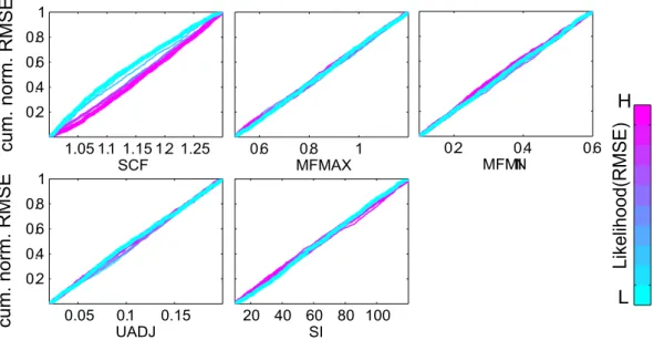
As described in Sect. 2.2.2, a visual extension of RSA (Young, 1978; Hornberger and Spear, 1981; Freer et al., 1996; Wagener and Kollat, 2007) was used to evaluate pa-rameter sensitivities for the SAC-SMA/SNOW-17 lumped model. Results were computed for the same timescales and watersheds as were presented for PEST. Given the large num-ber of results analyzed, Figs. 5 and 6 provide sample plots for our RSA analysis, whereas the full sensitivity classifications are summarized in Tables 5 and 6. In Figs. 5 and 6 each model parameter has its own plot with its range on the hori-zontal axis and its cumulative normalized RMSE distribution value on the vertical axis. In the plots, color shading is used to differentiate the likelihoods of each one of the ten bins used to divide the input parameter samples. High likelihood bins plotted in purple represent portions of the parameters’ ranges where low RMSE values are expected. In the con-text of sensitivity analysis, RSA measures the distribution of model responses that result from the 10 000 Latin hypercube input parameter groups sampled. When parameters are in-sensitive (see the SNOW-17 results shown in Fig. 5) each of the 10 sample bins plot over each other in linear trend lines that are representative of uniformly distributed RMSE values. Sensitive parameters produced highly dispersed bin lines such as those shown for LZTWM shown in Fig. 6.
cum. norm. RMSE
Likelihood(RMSE)
L
H
cum. norm. RMSE
1.05 1.1 1.15 1.2 1.25 0.2 0.4 0.6 0.8 1 SCF 0.6 0.8 1 MFMAX 0.2 0.4 0.6 MFMIN 0.05 0.1 0.15 0.2 0.4 0.6 0.8 1 UADJ 20 40 60 80 100 SI
Fig. 5. RSA (Regional Sensitivity Analysis) plot for Snow17 parameters in the SPKP1 watershed. The objective function is RMSE based
on a 1-hour time interval.
cum. norm. RMSE
Likelihood(RMSE)
L H
cum. norm. RMSE
cum. norm. RMSE
cum. norm. RMSE
20 40 60 80100 120 140 0.5 1 uztwm 20 40 60 80100 120140 0.5 1 uzfwm 0.2 0.3 0.4 0.5 1 uzk 0.02 0.04 0.06 0.08 0.5 1 pctim 0.1 0.2 0.3 0.5 1 adimp 50 100 150 200 0.5 1 zperc 2 4 0.5 1 rexp 200 400 0.5 1 lztwm 200 400 600 800 0.5 1 lzfsm 200 400 600 800 0.5 1 lzfpm 0.05 0.1 0.15 0.2 0.5 1 lzsk 0.005 0.01 0.015 0.02 0.5 1 lzpk 0.1 0.2 0.3 0.4 0.5 0.5 1 pfree
Fig. 6. RSA (Regional Sensitivity Analysis) plot for SAC-SMA parameters in the SPKP1 watershed. The objective function is RMSE based
Table 7. ANOVA single parameter sensitivities based on the RMSE measure. Dark gray shading designates highly sensitive parameters
defined using a threshold F value of 460. Light gray designates sensitive parameters defined using a threshold F value of 4.6. White cells in the table designate insensitive parameters. The values in the brackets provide the 95% confidence interval for the F-values (i.e., the unbracketed value ± the bracketed value yields the confidence interval).
Model Parameter SPKP1 SXTP1 1h 6h 24h 1h 6h 24h SCF 57.02 [21.78] 94.63 [27.57] 0.24 [2.40] 80.38 [25.71] 71.50 [23.80] 0.65 [2.79] MFMAX 0.64 [2.90] 1.79 [4.22] 1.27 [3.67] 1.40 [3.99] 1.15 [3.60] 1.03 [3.40] SNOW-17 MFMIN 1.51 [3.69] 13.52 [10.26] 178.03 [36.16] 0.25 [2.23] 19.53 [12.04] 9.96 [9.14] UADJ 1.25 [3.63] 1.76 [4.22] 0.86 [3.27] 1.18 [3.52] 1.01 [3.50] 1.89 [4.46] SI 1.25 [3.60] 0.03 [2.00] 9.94 [9.18] 5.27 [6.83] 7.58 [7.62] 1.83 [4.53] UZTWM 61.70 [23.35] 97.69 [27.41] 85.25 [26.54] 41.01 [17.68] 27.95 [14.84] 22.65 [14.04] UZFWM 57.14 [21.34] 22.91 [13.43] 44.90 [19.07] 31.87 [15.70] 64.83 [23.10] 119.42 [29.68] UZK 2.51 [4.83] 2.96 [5.06] 1.56 [3.98] 23.66 [13.23] 3.40 [5.33] 1.03 [3.33] PCTIM 123.52 [34.54] 463.48 [63.95] 232.04 [45.87] 107.64 [29.38] 121.19 [32.73] 9.81 [8.78] ADIMP 173.27 [42.48] 757.63 [82.30] 127.19 [33.93] 426.75 [60.13] 273.77 [50.98] 210.94 [46.35] ZPERC 11.91 [9.57] 18.38 [11.71] 9.59 [8.49] 64.16 [22.80] 30.37 [15.09] 9.79 [8.44] SAC-SMA REXP 7.81 [8.31] 7.77 [8.20] 8.23 [8.13] 19.62 [12.48] 13.86 [10.86] 7.36 [7.84] LZTWM 3047.02 [326.83] 3870.49 [255.63] 4025.30 [356.21] 1748.99 [143.26] 2722.24 [240.93] 1265.10 [199.25] LZFSM 54.29 [20.53] 22.75 [13.32] 51.53 [20.32] 12.46 [10.16] 33.93 [16.37] 36.64 [17.31] LZFPM 15.24 [11.28] 39.95 [17.75] 21.01 [13.16] 363.73 [56.37] 153.42 [35.83] 14.38 [10.67] LZSK 196.73 [39.09] 178.52 [36.40] 200.72 [39.07] 489.21 [66.64] 456.82 [62.66] 242.11 [48.62] LZPK 19.18 [11.97] 13.57 [10.32] 13.28 [10.26] 8.94 [8.55] 39.64 [17.31] 37.17 [17.45] PFREE 13.02 [10.35] 3.46 [5.53] 26.09 [14.49] 140.19 [31.35] 0.25 [2.44] 29.44 [16.21]
The SAC-SMA/SNOW-17 sensitivity classifications re-sulting from RSA are presented in Tables 5 and 6. The clas-sifications represent our qualitative interpretation of visual plots similar to those in Figs. 5 and 6 for each timescale and each watershed. As is standard in hydrologic applications of RSA (e.g., Freer et al., 1996; Wagener and Kollat, 2007), only individual parameter impacts on model performance are considered and parameter interactions have been neglected. Analysis of Tables 5 and 6 show changes in sensitivity when comparing across timescales, watersheds, and model perfor-mance objectives. Examples of these changes include the increased importance of the SNOW-17 parameters such as the mean water-equivalent above which 100-percent cover exists (SI) for the RMSE measure (i.e., high flow) and the minimum melt factor for non-rain periods (MFMIN) for the TRMSE measure (i.e., low flow) at the daily timescale. Both the RMSE measure and the TRMSE measure identified the vadose zone storage (LZTWM) as the most sensitive param-eter in all of the tested cases. Shifting the focus from high flow to low flow using the TRMSE measure resulted in the percolation factor (PFREE) and lower zone free water pri-mary maximum storage (LZFPM) being classified as being sensitive.
6.3 Sensitivity results for ANOVA
Recall that ANOVA is a parametric analysis of variance that uses the assumption of normally distributed model responses
(RMSE and TRMSE for streamflow in this study) to parti-tion variance contribuparti-tions between single parameters and parameter interactions. In this study, a second order ANOVA model (i.e., a model that considers pair wise parameter in-teractions) was fitted to the model outputs and the F-test is used to evaluate the statistical significance of each parame-ter’s or parameter interaction’s impact on the model output. Higher F-values indicate higher significance or sensitivity.
Additionally, the coefficient of determination r2can be used
to measure if incorporating parameter interactions into the ANOVA model improves its ability to represent model out-put variability (Mokhtari and Frey, 2005). Because random sampling can introduce significant uncertainty into the cal-culation of F-values, we have followed the recommendations of Archer et al. (1997) and used statistical bootstrapping to provide 95% confidence intervals for our ANOVA sensitivity rankings. Tables 7 and 8 provide F-values for each parameter as well as its bootstrapped confidence interval. Tabular pre-sentation of the ANOVA results improved their clarity since the F-values ranged over 4 orders of magnitude [0.25–4000] making plots difficult to interpret.
Tables 7 and 8 are formatted similarly to the prior sen-sitivity tables where highly sensitive parameters have dark grey shading, sensitive parameters have light grey shading, and insensitive parameters have no shading. These classifi-cations were based on the F-distribution where a threshold of 4.6 represents less than a 1-percent chance of
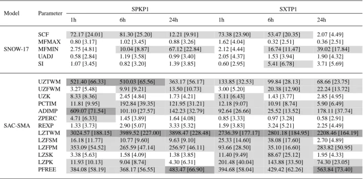
misclassi-Table 8. ANOVA single parameter sensitivities based on the TRMSE measure. Dark gray shading designates highly sensitive parameters
defined using a threshold F value of 460. Light gray designates sensitive parameters defined using a threshold F value of 4.6. White cells in the table designate insensitive parameters. The values in the brackets provide the 95% confidence interval for the F-values (i.e., the unbracketed value ± the bracketed value yields the confidence interval).
Model Parameter SPKP1 SXTP1 1h 6h 24h 1h 6h 24h SCF 72.17 [24.01] 81.30 [25.20] 12.21 [9.91] 73.38 [23.90] 53.47 [20.35] 2.07 [4.49] MFMAX 0.80 [3.17] 1.02 [3.45] 0.88 [3.26] 1.62 [4.04] 0.32 [2.51] 0.36 [2.51] SNOW-17 MFMIN 2.75 [4.81] 10.04 [8.87] 67.12 [22.84] 2.12 [4.44] 16.74 [11.47] 39.02 [17.84] UADJ 0.58 [2.84] 1.19 [3.58] 0.99 [3.40] 2.05 [4.37] 1.53 [3.94] 1.90 [4.32] SI 1.07 [3.45] 0.82 [3.20] 1.39 [3.85] 0.60 [2.95] 5.41 [6.78] 3.71 [5.69] UZTWM 521.40 [66.33] 510.03 [65.56] 363.17 [56.17] 133.85 [32.53] 99.84 [28.13] 68.66 [23.75] UZFWM 3.27 [5.48] 9.91 [9.21] 13.50 [10.73] 3.00 [5.20] 20.38 [12.90] 22.24 [13.72] UZK 8.33 [8.36] 2.45 [4.84] 1.73 [4.21] 5.11 [6.43] 1.43 [3.77] 2.85 [4.95] PCTIM 11.81 [9.95] 192.84 [39.35] 121.95 [31.21] 12.18 [9.07] 10.91 [8.74] 5.90 [6.49] ADIMP 609.07 [71.54] 101.10 [27.57] 142.23 [32.79] 92.64 [26.66] 25.52 [13.52] 178.11 [37.74] ZPERC 4.71 [6.33] 1.45 [3.89] 1.64 [4.08] 0.85 [3.33] 0.97 [3.28] 0.58 [2.91] SAC-SMA REXP 1.33 [3.73] 2.90 [5.07] 3.33 [5.32] 1.59 [3.83] 3.24 [5.21] 2.25 [4.49] LZTWM 3024.57 [188.15] 3989.52 [227.00] 3898.47 [228.48] 2736.39 [177.17] 2801.18 [184.95] 2208.46 [164.19] LZFSM 16.18 [11.77] 10.77 [9.60] 9.63 [9.10] 25.33 [14.60] 38.08 [17.60] 2.70 [4.89] LZFPM 353.09 [54.52] 265.59 [47.14] 256.97 [46.11] 93.66 [28.50] 35.10 [16.60] 283.82 [50.95] LZSK 3.38 [5.63] 1.58 [4.09] 1.38 [3.85] 11.40 [9.49] 88.67 [25.12] 1.95 [4.33] LZPK 11.93 [10.13] 9.04 [8.74] 4.30 [6.31] 201.48 [40.04] 143.88 [33.50] 74.30 [23.05] PFREE 384.08 [58.19] 368.17 [56.55] 483.47 [66.90] 394.68 [58.04] 429.42 [62.26] 563.84 [73.40]
fying a parameter as sensitive. As can be seen in the tables, some parameters’ F-values were up to three orders of magni-tude larger than 4.6. A threshold of 460 was used to classify parameters as being highly sensitive. Although the thresh-old used to classify highly sensitive parameters is subjec-tive, it accurately captures those parameters with very large F-values.
Analysis of Table 7 shows that for the high-flow RMSE objective, the most significant differences in sensitivities across timescales and across watersheds involved SNOW-17 parameters. The results show increasing sensitivities for the minimum melt factor for non-rain periods (MFMIN) at the 6-hour and daily timescales. Overall, Table 7 shows that most of the SAC-SMA parameters are sensitive for high flow con-ditions regardless of timescale or watershed. The high flow RMSE analysis identified the lower zone storage (LZTWM) as having the highest influence on model variance while the upper zone free water lateral depletion rate (UZK) is rated to have the least impact.
In Table 8 the ANOVA results using the low flow TRMSE objective are substantially different from those for high flow in Table 7. For low flow conditions, fewer parameters are classified as being sensitive. Table 8 shows a general reduc-tion relative to Table 7 in the influence of the upper zone free water storage (UZFWM) and an increase in the importance of the upper zone tension water storage (UZTWM) as well as the percolation factor (PFREE).
Beyond single parameter sensitivities, the coefficients of determination in Table 9 show that 2nd order interactions (or pairwise parameter interactions) improve the accuracy of the ANOVA model, which means the model better represents the total variance of the SAC-SMA/SNOW-17 model output. The coefficients of determination show that 2nd order param-eter interactions improve the ANOVA models’ performances by up to 40%. Figure 7 illustrates the 2nd order parame-ter inparame-teractions impacting the SAC-SMA/SNOW-17 model. Second order analysis changes the degrees of freedom used when analyzing the F-distribution making it necessary to de-fine a new threshold in Fig. 7. An F-value threshold of 3.32 designates at least a 99% likelihood of being sensitive. Again higher F-values imply higher sensitivity.
Figure 7 provides a more detailed portrayal of how pa-rameter sensitivities change across timescales for each of the watershed models. The RMSE results in Fig. 7a show that in-teractively sensitive parameters varied across watersheds as well as timescales. The results in Fig. 7b and Table 9 show that the SXTP1 watershed possesses more TRMSE-based ANOVA interactions than the SPKP1 watershed. The results imply each watershed model has a “unique” set of parameter interactions impacting its performance (Beven, 2000).
6.4 Sensitivity results for Sobol’s method
Recall from Sect. 2.2.4, that Sobol’s method decomposes the overall variance of the sampled SAC-SMA/SNOW-17 model
(a) (b) SC F M FM AX MFM IN UADJ SI UZTW M UZFW M UZK PC TI M ADIM P ZPER C REX P LZTW M LZFSM LZFP M LZSK LZPK PFREE Watershed: SPKP1 Time Interval: 1h SCF MFMAX MFMIN UADJ SI UZTWM UZFWM UZK PCTIM ADIMP ZPERC REXP LZTWM LZFSM LZFPM LZSK LZPK PFREE 0 50 100 150 SC F M FM AX MFM IN UA DJ SI UZ TW M UZ FW M UZ K PC TI M ADIM P ZPERCREX P LZTW M LZFSM LZFPMLZSK LZPKPFR EE Time Interval: 6h SCF MFMAX MFMIN UADJ SI UZTWM UZFWM UZK PCTIM ADIMP ZPERC REXP LZTWM LZFSM LZFPM LZSK LZPK PFREE 0 50 100 150 SC F MFM AX MFM IN UADJ SI UZTW M UZFW M UZK PC TI M ADIM P ZPERCR EXP LZ TW M LZ FSM LZFP M LZSK LZPK PFREE Time Interval: 24h SCF MFMAX MFMIN UADJ SI UZTWM UZFWM UZK PCTIM ADIMP ZPERC REXP LZTWM LZFSM LZFPM LZSK LZPK PFREE 0 50 100 150 SC F M FM AX MFM IN UA DJ SI UZTW M UZFW M UZK PC TIM ADIM P ZPER C REX P LZTW M LZFSM LZFP M LZSK LZPK PFREE Watershed: SXTP1 SCF MFMAX MFMIN UADJ SI UZTWM UZFWM UZK PCTIM ADIMP ZPERC REXP LZTWM LZFSM LZFPM LZSK LZPK PFREE 0 50 100 150 SC F M FM AX MFM IN UA DJ SI UZ TW M UZ FW M UZ K PC TIM ADIM P ZPER C REX P LZTW M LZFSM LZFPMLZSK LZPKPFR EE SCF MFMAX MFMIN UADJ SI UZTWM UZFWM UZK PCTIM ADIMP ZPERC REXP LZTWM LZFSM LZFPM LZSK LZPK PFREE 0 50 100 150 SC F MFM AX MFM IN UADJ SI UZTW M UZFW M UZK PCTI M ADIM P ZPERCR EXP LZ TW M LZ FSM LZFP M LZSK LZPK PFREE SCF MFMAX MFMIN UADJ SI UZTWM UZFWM UZK PCTIM ADIMP ZPERC REXP LZTWM LZFSM LZFPM LZSK LZPK PFREE 0 50 100 150 Sensitive SC F M FM AX MFM IN UA DJ SI UZTW M UZFW M UZK PC TI M ADIM P ZPER C REX P LZTW M LZFSM LZFP M LZSK LZPK PFREE Watershed: SPKP1 Time Interval: 1h SCF MFMAX MFMIN UADJ SI UZTWM UZFWM UZK PCTIM ADIMP ZPERC REXP LZTWM LZFSM LZFPM LZSK LZPK PFREE 0 20 40 60 80 100 SC F M FM AX MFM IN UA DJ SI UZ TW M UZ FW M UZ K PC TI M ADIM P ZPERCREX P LZTW M LZFSM LZFPMLZSK LZPKPFR EE Time Interval: 6h SCF MFMAX MFMIN UADJ SI UZTWM UZFWM UZK PCTIM ADIMP ZPERC REXP LZTWM LZFSM LZFPM LZSK LZPK PFREE 0 20 40 60 80 100 SC F MFM AX MFM IN UADJ SI UZTW M UZFW M UZK PCTI M ADIM P ZPERCR EXP LZ TW M LZ FSM LZFP M LZSK LZPK PFREE Time Interval: 24h SCF MFMAX MFMIN UADJ SI UZTWM UZFWM UZK PCTIM ADIMP ZPERC REXP LZTWM LZFSM LZFPM LZSK LZPK PFREE 0 50 100 150 SC F M FM AX MFM IN UA DJ SI UZTW M UZFW M UZK PC TI M ADIM P ZPER C REX P LZTW M LZFSM LZFP M LZSK LZPK PFREE Watershed: SXTP1 SCF MFMAX MFMIN UADJ SI UZTWM UZFWM UZK PCTIM ADIMP ZPERC REXP LZTWM LZFSM LZFPM LZSK LZPK PFREE 0 20 40 60 80 100 120 SC F M FM AX MFM IN UA DJ SI UZ TW M UZ FW M UZ K PC TI M ADIM P ZPER C REX P LZTW M LZFSM LZFPMLZSK LZPKPFR EE SCF MFMAX MFMIN UADJ SI UZTWM UZFWM UZK PCTIM ADIMP ZPERC REXP LZTWM LZFSM LZFPM LZSK LZPK PFREE 0 50 100 150 SC F MFM AX MFM IN UADJ SI UZTW M UZFW M UZK PC TI M ADIM P ZPERCR EXP LZ TW M LZ FSM LZFP M LZSK LZPK PFREE SCF MFMAX MFMIN UADJ SI UZTWM UZFWM UZK PCTIM ADIMP ZPERC REXP LZTWM LZFSM LZFPM LZSK LZPK PFREE 0 50 100 150 200 250 Sensitive
Fig. 7. (a) ANOVA second order parameter interactions based on the RMSE measure. (b) ANOVA second order parameter interactions
based on the TRMSE measure. Circles represent statistically significant F-values defined using the threshold value of 3.32. The color legends and shading represent the F-value magnitudes and ranges.
Table 9. Coefficients of determination for the ANOVA model. R1 designates a 1st order ANOVA model that neglects parameter interactions.
R2 designates a 2nd order ANOVA model that accounts for pairwise parameter interactions.
RMSE TRMSE
Order SPKP1 SXTP1 SPKP1 SXTP1
1h 6h 24h 1h 6h 24h 1h 6h 24h 1h 6h 24h
R1 0.535 0.755 0.643 0.601 0.604 0.543 0.745 0.739 0.718 0.556 0.546 0.541 R2 0.730 0.861 0.778 0.790 0.753 0.655 0.864 0.856 0.850 0.777 0.760 0.750
output to compute 1st order (single parameter), 2nd order (two parameter), and total order sensitivity indices. These in-dices are presented as percentages and have straightforward interpretations as representing the percent of total model out-put variance contributed by a given parameter or parameter interaction. The total order indices are the most comprehen-sive measures of a single parameter’s sensitivity since they represent the summation of all variance contributions involv-ing that parameter (i.e., its 1st order contribution plus all of its pairwise interactions).
Table 10 shows the relative importance of 1st and 2nd
or-der effects for all of the cases analyzed. Reaor-ders should note that the truncation and Monte Carlo approximations of the integrals required in Sobol’s method can lead to small nu-merical errors (e.g., see Archer et al., 1997; Sobol’, 2001; Fieberg and Jenkins, 2005) such as slightly negative indices or for example in Table 10 the few cases where 1st and 2nd order effects sum to be slightly larger than 1. In this study these effects were very small and did not impact parame-ter rankings. Table 10 supports our analysis assumption that 1st and 2nd order parameter sensitivities explain nearly all of the variance in the SAC-SMA/SNOW-17 model’s output distributions. The table also shows that the importance of 2-parameter interactions ranged from 3% to 40% of the total variance depending on the model performance objective, the prediction timescale, and the watershed. Except for SXTP1 6-hour test case, the results indicate that there were more pa-rameter interactions for the RMSE measure compared to the TRMSE measure.
Tables 11 and 12 summarize the total order indices (i.e., total variance contributions) for the SAC-SMA/SNOW-17 parameters analyzed. Again highly sensitive parameters are designated with dark grey shading, sensitive parameters have light grey shading, and insensitive parameters are not shaded. In all of the results presented for Sobol’s method, parameters classified as highly sensitive had to contribute on average at least 10-percent of the overall model variance and sensitive parameters had to contribute at least 1-percent. These thresh-olds are subjective and their ease-of-satisfaction decreases with increasing numbers of parameters or parameter inter-actions. In Tables 11 and 12 the total order indices again show that the model performance objective, the prediction timescale, and the watershed all heavily impact the SAC-SMA/SNOW-17 sensitivities.
In both tables, the SNOW-17 parameters contributed min-imally to the overall variance of the simulation model’s out-put. Only the minimum melt factor for non-rain periods (MFMIN) parameter has a statistically significant sensitivity when the bootstrapped confidence intervals are considered. Tables 11 and 12 also insinuate that most of the SAC-SMA model parameters are sensitive. For the high-flow RMSE re-sults, the lower zone tension water storage (LZTWM) and the additional impervious area (ADIMP) were the most sensitive SAC-SMA parameters. The upper zone storage parameters (UZTWM, UZFWM) and all of the lower zone parameters dominate model response for the low-flow TRMSE measure. In particular, the lower zone tension water storage (LZTWM) appears to be the dominant overall parameter as it explains about 50% of the output’s variance for each test case. Simi-lar to ANOVA’s results, there are fewer parameters classified as being sensitive for the TRMSE measure versus RMSE.
Figure 8 provides a more detailed understanding of the to-tal order indices presented in Tables 11 and 12. Similar to the ANOVA interaction plots in Section 6.3, these figures show the matrix of parameter interactions where circles designate pairings that contribute at least 1% of the overall model out-put variance. The actual 2nd order indices’ values are shown with the color shading defined in the plots’ legends. These plots show how the dominant parameters for both the RMSE and TRMSE measures tend to have the greatest number of interactions (e.g., LZTWM and PFREE in Fig. 8). Inter-estingly, there are very distinct differences for the param-eter interactions for the two watersheds. When comparing the RMSE results in Fig. 8a with TRMSE results in Fig. 8b the shift from high-flow to low flow analysis tends to sub-stantially decrease the importance of parameter interactions for the SPKP1 watershed, whereas no signification reduction was found for the SXTP1 watershed. Readers should note that our 1% threshold for Sobol’s method is particularly con-servative when analyzing Figs. 8a and b since the number of variables analyzed increases from 18 for 1st order analysis to 162 parameter interactions in 2nd order analysis.
6.5 Comparative summary of sensitivity methods
Sections 6.1-6.4 present classifications of
SAC-SMA/SNOW-17 model parameters into three categories: (1) highly sensitive, (2) sensitive, and (3) insensitive. Given