Systematic analysis of interannual and seasonal variations of model-simulated tropospheric NO<sub>2</sub> in Asia and comparison with GOME-satellite data

(1)

HAL Id: hal-00302259

https://hal.archives-ouvertes.fr/hal-00302259

Submitted on 10 Nov 2006

HAL is a multi-disciplinary open access

archive for the deposit and dissemination of sci-entific research documents, whether they are pub-lished or not. The documents may come from teaching and research institutions in France or abroad, or from public or private research centers.

L’archive ouverte pluridisciplinaire HAL, est destinée au dépôt et à la diffusion de documents scientifiques de niveau recherche, publiés ou non, émanant des établissements d’enseignement et de recherche français ou étrangers, des laboratoires publics ou privés.

Systematic analysis of interannual and seasonal

variations of model-simulated tropospheric NO2 in Asia

and comparison with GOME-satellite data

I. Uno, Y. He, T. Ohara, K. Yamaji, J.-I. Kurokawa, M. Katayama, Z. Wang,

K. Noguchi, S. Hayashida, A. Richter, et al.

To cite this version:

I. Uno, Y. He, T. Ohara, K. Yamaji, J.-I. Kurokawa, et al.. Systematic analysis of interannual and seasonal variations of model-simulated tropospheric NO2 in Asia and comparison with GOME-satellite data. Atmospheric Chemistry and Physics Discussions, European Geosciences Union, 2006, 6 (6), pp.11181-11207. �hal-00302259�

(2)

ACPD

6, 11181–11207, 2006 Analysis of interannual variations tropospheric NO₂in Asia I. Uno et al. Title Page Abstract Introduction Conclusions References Tables Figures J I J I Back Close

Full Screen / Esc

Printer-friendly Version

Interactive Discussion Atmos. Chem. Phys. Discuss., 6, 11181–11207, 2006

www.atmos-chem-phys-discuss.net/6/11181/2006/ © Author(s) 2006. This work is licensed

under a Creative Commons License.

Atmospheric Chemistry and Physics Discussions

Systematic analysis of interannual and

seasonal variations of model-simulated

tropospheric NO

₂

in Asia and comparison

with GOME-satellite data

I. Uno1, Y. He2, T. Ohara3, K. Yamaji4, J.-I. Kurokawa3, M. Katayama3, Z. Wang5, K. Noguchi6, S. Hayashida6, A. Richter7, and J. P. Burrows7

1

Research Institute for Applied Mechanics, Kyushu University, Kasuga Park 6-1, Kasuga, Fukuoka, Japan

2

Earth System Science and Technology, Kyushu University, Kasuga Park 6-1, Kasuga, Fukuoka, Japan

3

National Institute for Environmental Studies, Tsukuba, Ibaraki, Japan

4

Frontier Research Center for Global Change, Japan Agency for Marine-Earth Science and Technology, Yokohama, Japan

5

NZC/LAPC, Institute of Atmospheric Physics, Chinese Academy of Sciences, Beijing, China

6

Information Science, Faculty of Science, Nara Women’s University, Nara, Japan

7

Institute of Environmental Physics, University of Bremen, Bremen, Germany

Received: 14 September 2006 – Accepted: 7 November 2006 – Published: 10 November 2006

Correspondence to: I. Uno (iuno@riam.kyushu-u.ac.jp)

(3)

ACPD

Full Screen / Esc

Interactive Discussion Abstract

Systematic analyses of interannual and seasonal variations of tropospheric NO₂ ver-tical column densities (VCDs) based on GOME satellite data and the regional scale chemical transport model (CTM), Community Multi-scale Air Quality (CMAQ), are pre-sented over eastern Asia between 1996 and June 2003. A newly developed year-5

by-year emission inventory (REAS) was used in CMAQ. The horizontal distribution of annual averaged GOME NO₂VCDs generally agrees well with the CMAQ results. How-ever, CMAQ/REAS results underestimate the GOME retrievals with factors of 2–4 over polluted industrial regions such as Central East China (CEC), a major part of Korea, Hong Kong, and central and western Japan. For the Japan region, GOME and CMAQ 10

NO₂ data show good agreement with respect to interannual variation and show no clear increasing trend. For CEC, GOME and CMAQ NO₂ data show good agreement and indicate a very rapid increasing trend from 2000. Analyses of the seasonal cycle of NO₂VCDs show that GOME data have systematically larger dips than CMAQ NO₂ during February–April and September–November. Sensitivity experiments with fixed 15

emission intensity reveal that the detection of emission trends from satellite in fall or winter have a larger error caused by the variability of meteorology. Examination during summer time and annual averaged NO₂VCDs are robust with respect to variability of meteorology and are therefore more suitable for analyses of emission trends. Analysis of recent trends of annual emissions in China shows that the increasing trends of 1996– 20

1998 and 2000–2002 for GOME and CMAQ/REAS show good agreement, but the rate of increase by GOME is approximately 10–11% yr−1 after 2000; it is slightly steeper than CMAQ/REAS (8–9% yr−1). The greatest difference was apparent between the years 1998 and 2000: CMAQ/REAS only shows a few percentage points of increase, whereas GOME gives a greater than 8% yr−1 increase. The exact reason remains un-25

clear, but the most likely explanation is that the emission trend based on the Chinese emission related statistics underestimates the rapid growth of emissions.

(4)

ACPD

Full Screen / Esc

Interactive Discussion 1 Introduction

Examination of long-term tropospheric NO₂variation plays an important role in analysis of recent increases of NO_xemissions over Asia. As the NO₂lifetime is short and the ef-fects of horizontal transport in the continental boundary layer are small, it is reasonable to discuss the relationship between NO_x emission inventory and satellite NO₂vertical 5

column densities (VCDs). Richter et al. (2005) warned of the impact of rapid emission increases over China based on their Global Ozone Monitoring Experiment (GOME) satellite-derived NO₂columns. They show that the trend of increase is approximately of the order of 7% yr−1 from 1996 to 2002, implying an almost 40% increase within seven years. At the same time, GOME NO₂ columns show little variation in other ar-10

eas and agree well with ground-based measurements (Irie et al., 2005). Quite similar results were also recently reported by a study including both GOME and SCanning Imaging Absorption spectrometer for Atmospheric CHartographY (SCIAMACHY) data in a statistical analysis by van der A et al. (2006). However, as discussed by Richter et al. (2005) and van Noije et al. (2006), the GOME retrieval is very sensitive to several 15

factors including cloud screening and other chemical/meteorological conditions. Systematic comparison of satellite NO₂VCDs and application of the chemical trans-port model (CTM) plays an imtrans-portant role for emission analysis to overcome such difficulties. van Noije et al. (2006) presented a systematic comparison of NO₂columns from 17 global CTMs and three state-of-the-art GOME retrievals for the year 2000. 20

They report that, on average, the models underestimate the retrievals in industrial re-gions such as Europe, the eastern United States, and eastern China. They concluded that top-down estimations of NO_x emissions from satellite retrieval are strongly depen-dent on the choice of model and retrieval. These results are based on global CTMs with coarse horizontal resolution, whereas a regional CTM can have much finer resolu-25

tion, which is suitable for the resolution of recent emission inventories. As an example of a regional CTM application, Ma et al. (2006) compared the GOME-NO₂VCDs with MM5/RADM regional model simulations for July 1996 and 2000 based on the emission

(5)

ACPD

Full Screen / Esc

Interactive Discussion inventory of Streets et al. (2003) for the year 2000 and the Chinese Ozone Research

Programme (CORP) emission estimates for the year 1995 and questioned the accu-racy of emission inventories. However, their studies are restricted to July of those two years; no inter-annual variation is discussed.

The GOME retrieval (top-down approach) provides long-term data for almost 7 years 5

(January 1996–June 2003) and CTM studies corresponding to that period with year-by-year emission estimates are absolutely necessary as a bottom-up analysis. GOME data can provide constrains for the inverse method of emission estimates (e.g., Martin et al., 2003; Jaegl ´e et al., 2005). They also provide recent emission trends, but such a long-term CTM study has not yet been reported for Asia. As successful applications 10

for Asian air quality studies, the community multi-scale air quality model (CMAQ; Byun and Ching, 1999) has been used intensively by Zhang et al. (2002), Uno et al. (2005), Tanimoto et al. (2005), and Yamaji et al. (2006a). Here we report the results of a systematic analysis of seasonal and interannual variations of NO₂ VCDs based on GOME data and the regional scale CTM, CMAQ, and sensitivity experiments with the 15

latest emission inventory in Asia from 1996 to 2003.

2 Outline of CMAQ simulation, emission inventory and GOME retrieval

In the following, we will briefly describe the regional chemical transport model, the emission inventory, the GOME NO₂ retrievals and the settings used in the numerical experiments in this paper.

20

(a) Chemical Transport Model, CMAQ

The three-dimensional regional-scale CTM used in this study was developed jointly by Kyushu University and the National Institute for Environmental Studies (Uno et al., 2005) based on the Models-3 CMAQ (ver. 4.4) modeling system released by the US EPA (Byun and Ching, 1999). Briefly, the model is driven by meteorological 25

(6)

ACPD

Full Screen / Esc

Interactive Discussion fields generated by the Regional Atmospheric Modeling System (RAMS; Pielke et al.,

1992) with initial and boundary conditions defined by NCEP reanalysis data (2.5◦ res-olution and 6 h interval). The horizontal model domain for the CMAQ simulation is 6240×5440 km2 on a rotated polar stereographic map projection centered at 25◦N, 115◦E with 80×80 km2 grid resolution (see Fig. 1 of Tanimoto et al., 2005). For verti-5

cal resolution, 14 layers are used in the sigma-z coordinate system up to 23 km, with about seven layers within the boundary layer below 2 km. The SAPRC-99 scheme (Carter et al., 2000) is applied for gas-phase chemistry, and the AERO3 module for aerosol calculation.

(b) REAS emission inventory 10

Reliable emission inventories of air pollutants are becoming increasingly important to assess heavy air pollution problems in Asia. An emission inventory in Asia was re-ported for the TRACE-P and ACE-Asia field study by Streets et al. (2003) with 1◦×1◦ resolution. A similar global emission inventory is provided in the EDGAR database (Olivier et al., 2002). Recently, the Regional Emission inventory in Asia (REAS; Ohara 15

et al., 20061; Akimoto et al., 2006; Yamaji, 2006b) was constructed based on energy data, emissions factors, and other socio-economic information between the years 1980 and 2003. It provides an Asian emission inventory for ten chemical species: NO_x, SO₂, CO, CO₂, nitrous oxide (N₂O), NH₃, black carbon (BC), organic carbon (OC), methane (CH₄), and non-methane volatile organic compounds (NMVOC) from anthropogenic 20

sources (combustion, non-combustion, agriculture, and others). All emission species from each source sector have been estimated based on activity data on the district levels for Japan, China, India. South Korea, Thailand and Pakistan. For those other countries, estimations are based on activity data of the national level. The emissions

1

Ohara, T., Akimoto, H., Kurokawa, J., et al.: Asian emission inventory for anthropogenic emission sources between 1980 and 2020, in preparation, available athttp://www.jamstec.go.

jp/forsgc/research/d4/emission.htm, 2006.

(7)

ACPD

Full Screen / Esc

Interactive Discussion estimated for district and country level were distributed into a 0.5◦×0.5◦grid using index

data bases of population, location of large point source (LPS), road networks, and land coverage information.

REAS NO_x emission inventories considered the fossil fuel and biofuel combustion, biomass burning and soil. REAS Soil NOx emission (sum of N-fertilized soil and natural 5

soil) is estimated to be 400–500 GgN yr−1from China, which is approximately 12–15% of combustion base NO_x and highly uncertain, so in this study we do not include the soil NO_xemission in the CMAQ simulation.

The NO_x emission intensity (combustion base) of REAS version 1.1 for 2000 was estimated as 11.2 Tg-NO₂yr−1for all of China (27.3 Tg-NO₂for Asia). A similar number 10

of 10.5 Tg-NO₂yr−1 was reported from TRACE-P (Streets et al., 2003), and 13.8 Tg-NO₂·yr−1from EDGAR ver. 3.2.

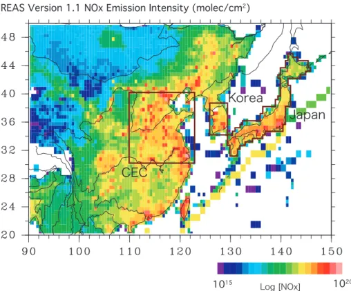
Figure 1 presents the horizontal distribution of REAS NO_xemissions for 2000 using log-scale coloring. Figure 1 shows that large NO_x emission regions are located in China (especially Hong-Kong, Shanghai, the North China Plain, and Beijing), Seoul, 15

Pusan, Taiwan, and central and western parts of Japan. The horizontal distribution and location of hot spots are very similar to those shown by TRACE-P emission inventory by Streets et al. (2003). The square region is CEC, and REAS NO_xemission within the CEC region are estimated at 4.86 Tg-NO₂yr−1, which corresponds to 43% of the total NO_xemission in China.

20

(c) GOME tropospheric NO₂Vertical Column Densities (VCDs)

GOME is a passive remote sensing instrument on board the ERS-2 satellite launched in April 1995. The GOME instrument observes the atmosphere at 10:30 local time (LT) and global coverage is achieved every 3 days with a footprint of 40 km latitude by 320 km longitude. For this study, we use the most recent version (ver. 2) of tropospheric 25

NO₂column data products retrieved by the University of Bremen (Richter et al., 2005). The retrieval version 2 data is based on 3-D CTM, SLIMCAT data, to exclude the

(8)

strato-ACPD

Full Screen / Esc

Interactive Discussion spheric NO₂ contribution, monthly AMF (air mass factor) evaluated with NO₂ profiles

from a run of the global model MOZART-2 for 1997 and a surface reflectivity climatology data. This version 2 retrieval accounts for aerosol based on three different scenarios taken from the LOWTRAN database (marine, rural and urban) distributed according to surface type and CO₂emissions. However, it does not include the effect of Asian dust 5

or any seasonal variability. Furthermore, no trend in aerosol is assumed. An increase in reflecting aerosols (e.g. sulfate) might result in higher sensitivity of GOME to NO₂ within and above the aerosol layers, possibly enhancing the observed trend (Richter et al., 2005; van der A et al., 2006; Martin et al., 2003). The intercomparison by van Noije et al. (2006) reported that the GOME NO₂retrieval by the University of Bremen gives a 10

slightly higher value over the Chinese winter (for 2000) when compared with two other retrievals (BIRA/KNMI and Dalhousie/SAO).

A rough estimate of the GOME NO₂ errors is an additive error of 0.5– 1.0×1015molecule cm−2 and a relative error of 40–60% over polluted areas. In ad-dition, the uncertainty for the annual average is approximately 15% (e.g. Richter et al., 15

2005).

For this study, the GOME tropospheric NO₂ swath data (ver. 2) files giving the lo-cation and value for each measurement pixel are all interpolated into a 0.5◦×0.546◦ longitude-latitude map (as with the REAS grid resolution). The GOME tropospheric NO₂data for the period of January 1996–June 2003 are used in this study.

20

(d) Setting of numerical experiments by CMAQ/REAS

In this study, an eight-full-year simulation was conducted for 1996–2003. For this CMAQ modeling system, all emissions were obtained from 0.5◦×0.5◦resolution of the REAS ver. 1.1 database. The effect of seasonal dependence of emissions were ex-amined by Streets et al. (2003), and they indicated that domestic space-heating com-25

ponent has a seasonality and the ratio of monthly emissions was approximately 1.2 between maxima and minima (see Fig. 7 of Streets et al., 2003). However, the speci-fication of emission seasonality is very difficult, so emission intensity for the CMAQ is

(9)

ACPD

Full Screen / Esc

Interactive Discussion set as constant for each year and no seasonal variation is assumed. The initial fields

and monthly averaged lateral boundary condition for most chemical tracers are pro-vided from a global chemical transport model (CHASER; Sudo et al., 2002). This fixed lateral boundary condition is used for the eight-full-year simulation (i.e., no interannual variation of lateral conditions is assumed). The CMAQ output data are all interpolated 5

to 0.5◦×0.5◦ resolution of REAS to facilitate an easy comparison.

Two sets of numerical experiments were conducted. Series E00Myy simulations used the fixed emission for 2000 with year-by-year meteorology. Series EyyMyy use both year-by-year emissions and meteorology. These two experiments were set to elucidate the sensitivity for both meteorology and changes in emission intensity. The 10

GOME measurements in low latitudes and middle latitudes are always taken at the same LT (approximately 10:30 LT). Therefore, we used the CMAQ output of 03:00 UTC (11:00 LT for China and 12:00 LT for Japan) for comparison.

3 Results and discussion

3.1 General distribution and comparison of NO₂in Asia for 2000 15

We will show a general comparison of CMAQ NO₂ VCDs and GOME retrieval results. To obtain the CMAQ simulated tropospheric NO₂ VCDs, we integrated the column NO₂loading from surface to 10 km height. No seasonal variation of tropopause height is considered because approximately 95% of NO₂ resides at heights below 3 km in the CMAQ simulation and the same lateral boundary condition is used for all model 20

experiments. We set three regions in central east China (CEC; 30◦N, 110◦E to 40◦N, 123◦E), Korea and Japan to produce detailed comparisons (see Fig. 1). The definition of CEC is the same area used by Richter et al. (2005).

The GOME observations are strongly sensitive to cloud cover (only retrieved when cloud cover is less 0.2). Their observations are only taken every 3 days. To make 25

(10)

inter-ACPD

Full Screen / Esc

Interactive Discussion est. Satellite Region Average (SRA) is the average of CMAQ NO₂ VCDs for exactly

the same timing and grid point as the GOME observation, which is most suitable for comparison with satellite data. Another average is the simple region average without any consideration of GOME observation timing; this we call as the simple CTM Region Average (CRA). The difference between SRA and CRA gives an indication on the ob-5

servation bias of GOME retrievals as result of the measurement sampling and cloud selection.

Figure 2 shows (a) the annual mean CMAQ simulated tropospheric NO₂VCDs aver-aged by SRA for year the 2000, (b) the annual mean GOME satellite data for the year 2000, and (c) the difference of CMAQ and GOME (a–b). Figure 3 shows (a) scatter 10

plots between REAS NO_xemission and NO₂VCDs of CMAQ and GOME excluding the ocean area, and (b) scatter plots between CMAQ NO₂ VCDs and GOME retrieval for all grid points.

The lifetime of NO₂is short. Therefore, CMAQ simulated NO₂VCDs (Fig. 2a) shows a quite similar distribution with the REAS NO_x emission map (Fig. 1). Annual mean 15

GOME NO₂ VCDs (shown in Fig. 2b) and the difference to the CMAQ NO₂ VCDs (Fig. 2c) provide important information related to Asian NO_x emissions. High GOME NO₂VCDs regions generally agree with the CMAQ (and REAS) results. The difference between CMAQ and GOME (Fig. 2c) indicates that the CMAQ results underestimate the GOME retrievals over polluted industrial regions such as CEC, a major part of 20

Korea, Hong-Kong, and central and western Japan. It is noteworthy that CMAQ shows a high concentration over Taiwan, two large cities in Korea (Seoul and Pusan) and northeastern China (e.g., the region between Shenyang and Changchun), which are not strongly identified in GOME data mainly due to the strong longitudinal averaging of GOME data.

25

A more detailed analysis of the NO_x emissions, GOME retrieval and CMAQ NO₂is presented in Fig. 3. Figure 3a shows the relationship between REAS NO_x emission (converted to molecule cm−2) and NO₂ VCDs over the land surface, respectively, by GOME (blue) and CMAQ (red). The GOME NO₂value has a clear cut-off at the level

(11)

ACPD

Full Screen / Esc

Interactive Discussion of 0.5×1015molecule cm−2. This figure indicates the responses of emission to the

atmospheric concentrations for the model and GOME. The data points are scattered widely. Nevertheless, the expected linear increasing relationship is visible.

Finally, Fig. 3b) shows the systematic under-estimation of CMAQ NO₂for all grid points. Most CMAQ NO₂ VCDs are distributed between y=x and y=3x (i.e. factor 5

3 range). The red squares indicate grid points within the CEC region, blue triangles are used for Korea, green squares for Japan, and yellow dots for data from west of 105◦E. All other data are shown as gray dots. As this figure shows, most Japanese data are located around the line between y=x and y=3x, which is a fundamentally identical pattern to that obtained using CEC data (even if some CEC data are located 10

near the y=4x line), whereas most Korean data are located between y=2x and y=3x. Because the GOME retrieval gives NO₂ VCDs as a response of NO_x emission based on the unified retrieval algorithm, this close examination with CMAQ NO₂ shows that some of emission inventory data distributed outside the general pattern might require re-examination of the basic energy consumption, emission factors, and socio-economic 15

data used for the construction of the emission inventory.

For the low emission region (intensity below 1017molecule cm2) shown in Fig. 3a, GOME and CMAQ responses are different: GOME is systematically higher than CMAQ. This is mainly attributable to the effect of biomass burning. The contribution of biomass burning NO₂is higher in these regions, whereas the REAS emission inven-20

tory for biomass burning is taken from TRACE-P emission inventory and is different for 2000. An almost identical result is pointed out by Ma et al. (2006). It is also important to point out that the gray dot points below 0.6×1015molecule cm−2 (shown in Fig. 3b) are mainly over the ocean and show an almost 1:1 relationship between GOME and CMAQ VCDs.

(12)

ACPD

Full Screen / Esc

Interactive Discussion 3.2 Analysis of interannual and seasonal variations of NO₂

The evolution of the tropospheric columns of NO₂above the regions of Japan and CEC (see in Fig. 1) are shown in Fig. 4. The thick red line represents the monthly averaged GOME NO₂ VCDs. The figure also includes results of CMAQ E00Myy SRA (thick-green), EyyMyy SRA (thick-black dotted line), and EyyMyy CRA (thin-dashed-black 5

line). The gray vertical line is the daily averaged value from E00Myy CRA in order to show the range of day-by-day variation of simulated concentration. GOME and SRA average data are only shown until June 2003 because of data availability. Because the CMAQ underestimates the GOME retrieval, the vertical axis for CMAQ (right axis) is adjusted to improve the view.

10

First, for the Japan region (Fig. 4a), GOME retrieval and CMAQ EyyMyy SRA show good agreement and no clear increase, which is consistent with the REAS emission inventory for Japan that shows no clear increasing trend (the REAS variation is less than ±2% during 1996–2003). The best fitting line based on all yearly data is

GOME NO₂= –5.55E14 + 2.41 × CMAQ NO₂(molecule cm2) (R=0.919). 15

The CMAQ values are approximately 40% that of GOME. Data for February 2001 are not used because only one observation day was available. The exact reason why the CMAQ underestimates the GOME VCDs remains unclear; however, the high correla-tion supports that the combinacorrela-tion of CMAQ and GOME results is suitable for analysis of the interannual and seasonal variation of NO₂concentration and emission trends. 20

The monthly means of GOME and CMAQ EyyMyy SRA are located within the daily variation line of E00Myy CRA, meaning that the emission trend does not increase from the estimate for 2000. The CMAQ results reproduce the seasonal variation very well, showing the summer (July–August) minimum and winter (December) maximum. Some differences pertain between SRA and CRA results, especially in winter (CRA is smaller 25

than SRA), which indicates the GOME retrieval has a slightly positive bias in Japan because of GOME’s observation on days with clear weather and the small number of observations in winter.

(13)

ACPD

Full Screen / Esc

Interactive Discussion The results for CEC (Fig. 4b) provide very important facts about China. First, the

general agreement between GOME and CMAQ looks similar to Japan. It is important to point out that GOME retrieval shows a strongly increasing trend during 2001–2003, but its trend is gentler during 1996 and 1999. For China, the result of EyyMyy SRA and EyyMyy CRA is almost identical, which is a result of the choice of a wide averaging 5

region (approximately 1000×1000 km2). Consequently, the monthly CRA result is also suitable for comparison with monthly mean GOME data for a wide region like CEC.

Several sensitivity lines in Fig. 4b are very interesting. The CMAQ E00Myy SRA (fixed emission for 2000) basically retrieves the interannual variation of GOME, but shows too high values before 1998, and too small values after 2002. That fact indi-10

cates that the NO_xemission is increasing year-by-year between 1996 and 2003, even considering the effect of meteorological variability. It is interesting that the results of E00Myy show good agreement with GOME NO₂ during 1999 and 2001, suggesting that emission increases during this period are small or that the variation of meteorol-ogy masks the trend; additional relevant details will be discussed in Sect. 3.3. The 15

CMAQ results for EyyMyy (SRA and CRA are almost the same) reproduce well the increasing trend of the GOME columns from 1996 and 2003, especially the increasing trend of the summer time minimum value. We can see that the winter peak value of CMAQ NO₂ during 2002–2003 is smaller than that of GOME. The reason is unclear, but possible reasons will be addressed later in Sect. 3.3.

20

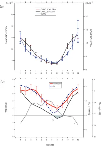
The seasonal variation in CEC is basically identical to that in Japan. Figure 5 shows seasonal variations of NO₂ VCDs for CMAQ and GOME. Here, seven-year averaged data for SRA are used for GOME and CMAQ NO₂ VCDs; the vertical axis is different for CMAQ and GOME. Error bars show the range from one standard deviation more to one less. The figure also shows the wind speed and water vapor mixing ratio, Q_v 25

over the CEC region from RAMS simulation. Wind speed and Q_v quantities are the respective averages of values at the surface and those at z=500 m.

Maximum values of the NO₂ columns occur in December even though the wind speed is higher. This indicates that the effect of the longer chemical lifetime of NO₂

(14)

ACPD

Full Screen / Esc

Interactive Discussion is more important than that of strong wind. While the minimum value is observed in

July and August because of the strong vertical mixing, the short lifetime of NO₂ and the inflow of relatively clean air from the Pacific Ocean side. At this minimum value, CMAQ VCDs corresponds to 64% of the value of GOME VCDs. This seasonal varia-tion is asymmetric and the slope (curvature) of the seasonal variavaria-tion of NO₂ both for 5

CMAQ and GOME is different during January–June and September–December. For this seasonal variation of NO₂, wind changes must play an important role; the variation of NO₂ and the east wind (U component) are well correlated. Because the east wind indicates the summer monsoon from the Pacific Ocean side and will bring fresh air, as indicated from the increase of Q_v. This east wind ceases in September (rapid stop of 10

summer monsoon) and changes to the west and north wind directions resulting in a rapid increase of NO₂levels.

Both CMAQ and GOME data show a large standard deviation during January–March and October–December, which shows that the variability of meteorology plays an im-portant role in these seasons. When comparing the scaled GOME and model NO₂ 15

variation, GOME retrievals during February–April and September–November shows larger dips (concave shape) than CMAQ, even when considering the error bar of the standard deviation. The exact reasons for this discrepancy are not yet clear and need more work both from the CTM side and satellite retrieval method.

3.3 Role of interannual variability of wind speed and analysis of recent trends of emis-20

sion intensity

The effect of interannual variability of meteorology (especially wind speed) plays an important role in determining the NO₂concentration level. Sensitivity experiments with fixed emission rate for 2000 (E00Myy) provide the effect of wind speed for NO₂ con-centration.

25

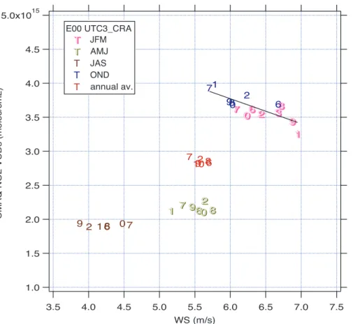
Figure 6 shows a scatter plot of three-month averaged CMAQ NO₂ VCDs and wind speed in the CEC region during 1996 and 2003. Wind speed below z=500 m is aver-aged in the figure. Three months averaver-aged and annual averaver-aged value are shown in

(15)

ACPD

Full Screen / Esc

Interactive Discussion different color and numbers show the last digit of the year (e.g., 9=1999 and 1=2001).

This analysis is important to show the effect of wind speed variability for the concen-tration level to analyze the GOME retrieval (i.e., observed data includes the effect of meteorological variability).

The figure shows that NO₂ VCDs are higher in winter (JFM) and fall (OND). It is 5

noteworthy that 1999 and 2001 in JFM have higher wind speeds. Furthermore, 1997 and 2000 in JFM have slower overall wind speeds and the difference is about 0.7– 1.0 m s−1(corresponding to 15% of magnitude). The difference of NO₂VCDs in 1997 and 2001 exceeded 0.3–0.4 molecule cm−2 (10%) compared to 1999 and 2001. The linear fitting result for OND and JFM is

10

CMAQ NO₂(molecule cm−2)= 5.976E15 – 3.671E14 × WS (m s−1) (R=–0.784). That result implies that the 10% difference in WS (around WS=6.5 m s−1) causes a 10% difference in NO₂VCDs. The detection of an emission trend from satellite (and/or surface monitoring stations) in fall or winter therefore results in a larger error because of the variability of meteorology.

15

For spring and summer seasons, NO₂ VCDs are smaller (40–50% of that of OND) and are not strongly sensitive to the change of wind speed (for AMJ, CMAQ NO₂ ranges 2.11-2.27E15 molecule cm−2 (approximately 7%). This characteristic is also valid for annual averages (ranges 2.82–2.92 molecule cm−2; approximately 3.5%). We conclude that the analysis of summer time and annual average NO₂VCDs is much less 20

sensitive to variability of meteorology and is suitable for the analysis of emission trends, even though it still includes the 3–7% variation arising form meteorological variability.

Another important analysis for recent emission increase in CEC was made in Fig. 7. This figure shows the scatter of monthly averaged NO₂ VCDs for GOME and CMAQ EyyMyy SRA. Red numbers represent data from CEC (last digit of the year). Blue 25

symbols are data from Japan. The best fit between GOME and CMAQ for CEC is CMAQ NO₂= 5.12E15 – 5.00E15 × exp [–1.45E–16 × GOME NO₂]

This fit indicates that GOME NO₂ is more enhanced when the CMAQ NO₂ concen-tration becomes higher (i.e., emission becomes higher); most of these conditions occur

(16)

ACPD

Full Screen / Esc

Interactive Discussion after the year 2000.

The exact reason why the relationship between CMAQ NO₂ and GOME NO₂ be-comes nonlinear remains unclear. However, several possible reasons include: (1) the estimated emissions do not reflect the recent NO_xemission increases enough, and (2) the basic assumptions (e.g., no aerosol trend or change in air mass factor, etc.) of 5

GOME NO₂retrieval require re-consideration. The assumption of no trend in aerosols might not be appropriate in China. The REAS SO₂ emission in China increases by about 30% between the year 2000–2003, which results in a CMAQ sulfate increase of 13% in CEC region. Detailed studies are necessary to better understand differences in recent NO₂trends between CMAQ and GOME.

10

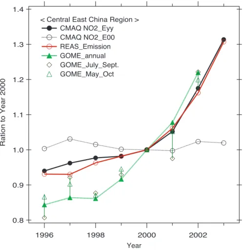
Our final and strongest interest is the understanding of the recent trend of emission increases in CEC. Figure 8 shows the trend of GOME NO₂, CMAQ NO₂and REAS NO_x emission normalized to 2000. To determine the annual average of GOME for 1998, the January 1997 value was used in place of the missing observation of Jan. 1998. The dashed line with an open circle shows the variation of E00Myy simulation (0.99–1.03), 15

which shows the effect of meteorological variability. The normalized result for CMAQ and REAS shows a very similar trend, indicating that CMAQ NO₂ VCDs responds to the NO_x emission trend with almost equivalent magnitude. A similar response for the MOZART model is also discussed in Richter et al. (2005).

As depicted in Fig. 6, GOME NO₂ is sensitive to the selection of season, so three 20

cases of average (simple annual average, average between May and October and between July and September (JAS)) are plotted. The green vertical bar shows the range of variation caused by the choice of averaging period of GOME; the error bar has an order of 5–10%.

An increasing trend of 1996–1998 and 2000–2002 for GOME and CMAQ/REAS 25

shows a good agreement, even though the GOME data give a slightly steeper trend after the year 2000 (GOME is approximately 10–11% yr−1, whereas CMAQ/REAS is 8–9% yr−1). The greatest difference also can be found between 1998 and 2000. The CMAQ/REAS result shows only a few percentage points of increase, but GOME gives

(17)

ACPD

Full Screen / Esc

Interactive Discussion more than 8% yr−1of increase. This 8% yr−1increase exceeds the possible estimation

error bar attributable to the meteorological variability (ca. 3–4%). Akimoto et al. (2006) and Zhang et al. (2006)2discussed the reliability of statistical reports from the Chinese government during this period. The most likely explanation is that the REAS emission trend (based on Chinese data) underestimates the rapid growth of emissions. This re-5

sult highlights that combinations of CTM based on bottom-up inventories with satellite top-down estimates can play an important role in improving emission inventory esti-mates and provide very useful information that advances the development of a reliable CTM simulation.

4 Conclusions

10

Systematic analyses of interannual and seasonal variations of tropospheric NO₂ ver-tical column densities (VCDs) based on GOME satellite data and the regional scale CTM, CMAQ, were presented over East Asia for the time period from January 1996 to June 2003. Numerical simulations with a year-by-year base of the REAS emission inventory in Asia during the same period were analyzed.

15

The main results are:

1) The horizontal distribution of annual averaged GOME NO₂VCDs for 2000 gener-ally agrees with CMAQ/REAS results. However, CMAQ results underestimate GOME retrievals by factors of 2–4 over polluted industrial regions such as Central East China (CEC), the major part of Korea, Hong-Kong, and central and western areas of Japan. 20

Examination of differences of GOME and CMAQ also suggested that the emission in-ventory of some regions (e.g., Taiwan, two large city region of Korea and northeastern China) demand re-examination.

2) Evolution of the tropospheric columns of NO₂ above Japan and CEC between 1996 and 2003 was examined. For the Japan region, GOME retrieval and CMAQ NO₂ 25

2

(18)

ACPD

Full Screen / Esc

Interactive Discussion show a good agreement and no clear increasing trend, which is consistent with the

REAS emission inventory for Japan. For CEC, the general agreement between GOME and CMAQ is also good. Both GOME and CMAQ NO₂ show a very sharp increasing trend after 2000. The seasonal cycle of NO₂ VCDs from both CMAQ and GOME is asymmetric because of the summer monsoon exchange from the Pacific Ocean side. 5

We also found that GOME retrievals during February–April and September–November have systematically larger dips (concave shape) than CMAQ, even considering their error bar.

3) A sensitivity experiment with a fixed emission rate for year 2000 shows that detec-tion of emission trends over CEC from satellite data in fall or winter result in larger errors 10

because of the variability of meteorology. Examination during summer and annual av-eraged NO₂VCDs is much less sensitive to variability of meteorology and suitability of analysis of emission trends, even though it still includes 3–7% of the variability coming from meteorological variability.

4) Recent trends of annual emission increases in CEC were examined. Increas-15

ing trends of 1996–1998 and 2000–2002 for GOME and CMAQ/REAS shows a good agreement, but the increasing rate of the GOME data is approximately 10–11% yr−1 af-ter 2000, slightly steeper than CMAQ/REAS (8–9% yr−1). The greatest difference was found between the years 1998 and 2000. The CMAQ/REAS shows only a few percent-age points of increase, while GOME gives more than 8% yr−1 of increase. The exact 20

reason remains unclear, but the most likely explanation is that the REAS emission trend (based on the Chinese statistics) underestimates the rapid growth of emissions during this time period.

Acknowledgements. This study was supported in part by funds from a Grant-in-Aid for

Scien-tific Research under Grant No. 17360259 from the Ministry of Education, Culture, Sports,

Sci-25

ence and Technology of Japan, and from the Steel Industry Foundation for the Advancement of Environmental Protection Technology (SEPT) and the European Union through ACCENT.

(19)

ACPD

Full Screen / Esc

Interactive Discussion References

Akimoto, H., Ohara, T., Kurokawa, J., and Horii, N.: Verification of energy consumption in China during 1996–2003 by satellite observation, Atmos. Env., in press, 2006.

Byun, D. W. and Ching, J. K. S. (Eds.): Science algorithms of the EPA Models-3 community multi-scale air quality (CMAQ) modeling system, NERL, Research Triangle Park, NC EPA/

5

600/R-99/030, 1999.

Carter, W. P. L.: Documentation of the SAPRC-99 chemical mechanism for VOC reactivity assessment, Final report to California Air Resource Board, Contract No. 92-329 and 95-308, May, 2000.

Irie, H., Sudo, K., Akimoto, H., et al.: Evaluation of long-term tropospheric NO2 data

10

obtained by GOME over East Asia in 1996–2002, Geophys. Res. Lett., 32, L11810, doi:10.1029/2005GL022770, 2005.

Jaegl ´e, L., Steinberger, L., Martin, R. V., and Chance, K.: Global partitioning of NO_x sources using satellite observations: Relative roles of fossil fuel combustion, biomass burning and soil emissions, Faraday Discuss., 130, 407–423, 2005.

15

Ma, J., Richter, A., Burrows, J. P., N ¨uß, H., and van Aardenne, J. A.: Comparison of model-simulated tropospheric NO₂over China with GOME-satellite data, Atmos. Environ., 40, 593– 604, 2006.

Martin, R. V., Jacob, D. J., Chance, K., Kurosu, T. P., Palmer, P. I., and Evans, M. J.: Global inventory of nitrogen oxide emissions constrained by space-based observations of NO₂

20

columns, J. Geophys. Res., 108, 4537, doi:10.1029/2003JD003453, 2003.

Olivier, J. G. J., Berdowslki, J. J. M., Peters, J. A. H. W., Visschedijk, A. J. H., Bekker, J., and Bloos, J. P. J.: Applications of EDGAR: Emission Database for Global Atmospheric Re-search. Dutch National Research Programme on Global Air Pollution and Climate Change, report no. 410 200 051, 2002.

25

Pielke, R. A., Cotton, W. R., Walko, R. L., Tremback, C. J., Lyons, W. A., Grasso, L. D., Nicholls, M. E., Moran, M. D., Wesley, D. A., Lee, T. J., and Copeland, J. H.: A comprehensive mete-orological modeling system—RAMS. Meteorol. Atmos. Phys., 49, 69–91, 1992.

Richter, A., Burrows, J. P., N ¨uß, H., Granier, C., and Niemeier, U.: Increase in tro-pospheric nitrogen dioxide over China observed from space, Nature, 437, 129–132,

30

doi:10.1038/nature04092, 2005.

(20)

Nel-ACPD

Full Screen / Esc

Interactive Discussion

son, S. M., Tsai, N. Y., Wand, M. Q., Woo, J.-H., and Yarber, K. F.: An inventory of gaseous and primary aerosol emissions in Asia in the year 2000, J. Geophys. Res., 108(D21), 8809, doi:10.1029/2002JD003093, 2003.

Sudo, K., Takahashi, M., Kurokawa, J., and Akimoto, H.: CHASER: a global chemical model of the troposphere – 1. Model description, J. Geophys. Res.-Atmos., 107(D17), 4339,

5

doi:10.1029/2001JD001113, 2002.

Tanimoto, H., Sawa, Y., Matsueda, H., Uno, I., Ohara, T., Yamaji, K., Kurokawa, J., and Yone-mura, S.: Significant latitudinal gradient in the surface ozone spring maximum over East Asia, Geophys. Res. Lett., 32, L21805, doi:10.1029/2005GL023514, 2005.

Uno, I., Ohara, T., Sugata, S., Kurokawa, J., Furuhashi, N., Yamaji, K., Tanimoto, N.,

Yumi-10

moto, K., and Uematsu, M.: Development of RAMS/CMAQ Asian scale chemical transport modeling system, J. Japan Soc. Atmos. Environ., 40(4), 148–164 [in Japanese], 2005. van Noiji, T. P. C., Eskes, H. J., Dentener, F. J., et al.: Multi-model ensemble simulations of

tropospheric NO₂compared with GOME retrievals for the year 2000, Atmos. Chem. Phys., 6, 2943–2979, 2006.

15

van der A, R. J., Peters, D. H. M. U., Eskes, H., Boersma, K. F., Van Roozendael, M., De Smedt, I., and Kelder, H. M.: Detection of the trend and seasonal variation in tropospheric NO₂over China, J. Geophys. Res., 111, D12317, doi:10.1029/2005JD006594, 2006.

Yamaji, K., Ohara, T., Uno, I., Tanimoto, H., Kurokawa, J., and Akimoto, H.: Analysis of seasonal variation of ozone in the boundary layer in East Asia using the Community Multi-scale Air

20

Quality model: What controls surface ozone level over Japan?, Atmos. Environ., 40, 1856– 1868, 2006a.

Yamaji, K.: Modeling study of spatial-temporal variations of tropospheric ozone over East Asia, Ph. D. thesis for Kyushu University, 2006b.

Zhang, M.-G., Uno, I., Sugata, S., Wang, Z.-F., Byun, D. W., and Akimoto, H.: Numerical

25

study of boundary layer ozone transport and photochemical production in east Asia in the wintertime, Geophys. Res. Lett., 29, doi:10.1029/2001GL014368, 2002.

(21)

ACPD

Full Screen / Esc

Interactive Discussion REAS Version 1.1 NOx Emission Intensity (molec/cm2₎

CEC

Korea

Japan

1015 ₁₀20

Log [NOx]

Fig. 1. Horizontal distribution of REAS NO_x emission for year 2000. Square regions are aver-age areas used for detailed analyses.

(22)

ACPD

Full Screen / Esc

Interactive Discussion (a) CMAQ NO2 VCDs for year 2000 (molec/cm2₎

Fig. 2 (Uno et al.)

(b) GOME NO2 VCDs for year 2000 (molec/cm2₎

(c) Difference between CMAQ and GOME NO2 VCDs [ (a)-(b) ]

Fig. 2. (a) Annual mean CMAQ simulated tropospheric NO₂VCDs averaged by SRA for year 2000,(b) Annual mean GOME satellite data for year 2000 and (c) the difference of CMAQ and

GOME (a–b).

(23)

ACPD

Full Screen / Esc

(a) Scatter of REAS NOx Emission and (CMAQ and GOME NO2 VCDs)

1014 2 3 4 5 6 7 8 9 1015 2 3 4 5 6 7 8 9 1016 2 3 NO2 VCDs (molec/cm 2) 1015 1016 1017 1018 1019 1020 REAS NOx Emission (molec/cm2)

CMAQ GOME

over land

Fig. 3 (Uno et al.) (b) Scatter of CMAQ and GOME NO2 VCDs

1014 2 3 4 5 6 7 8 1015 2 3 4 5 6 7 8 1016 2

GOME NO2 VCDs (molec/cm2)

1014 2 3 45 6 7 1015 2 3 45 6 7 1016 2 CMAQ NO2 VCDs (molec/cm2) West of 105E China_CEC Region Japan Korea y=x y=2x y=4x y=3x

Fig. 3. (a) Scatter plots between REAS NO_x emission and NO₂ VCDs excluding the ocean area for the year 2000 and(b) scatter plots between annual averaged CMAQ NO₂ VCDs and GOME retrieval for all grid points (shown by grey points except for the points indicated in the figure).

(24)

ACPD

Full Screen / Esc

Printer-friendly Version Interactive Discussion 7x1015 6 5 4 3 2

CMAQ NO2 VCDs (molcu/cm2)

2004 2003 2002 2001 2000 1999 1998 1997 1996 Yearr 25x1015 20 15 10 5 0

GOME CMAQ E00_SRA CMAQ Eyy_SRA CMAQ Eyy_CRA E00_daily_CRA

Central East China Region (Monthly averaged data analysis) (b) Central East China

8x1015

6

4

2

CMAQ NO2 VCDs (molcu/cm2)

2004 2003 2002 2001 2000 1999 1998 1997 1996 Yearr 25x1015 20 15 10 5 0

GOME CMAQ E00_SRA CMAQ Eyy_SRA CMAQ Eyy_CRA E00_daily_CRA

Central Japan Region (Monthly averaged data analysis)

(a) Japan

Fig. 4 (Uno et al.)

Fig. 4. Evolution of the tropospheric columns of NO₂over the region of(a) Japan and (b) CEC.

The thick red line represents the monthly averaged GOME NO₂ VCDs, and thick-green line is CMAQ E00Myy SRA, thick-black dotted line is EyyMyy SRA and thin-dashed-black line is EyyMyy CRA. The gray vertical line shows the daily averaged value from CMAQ E00Myy CRA. (SRA is the Satellite Region Average, and CRA is the simple CTM Region Average. E00Myy simulation used the fixed emission for 2000 with year by year meteorology, and EyyMyy use both year-by-year emission and meteorology).

(25)

ACPD

Full Screen / Esc

Interactive Discussion Fig. 5 (Uno et al.)

7x1015 6 5 4 3 2 CMAQ NO2 VCDs 12 11 10 9 8 7 6 5 4 3 2 1 MONTH 25x1015 20 15 10 5 0 GOME NO2 VCDs CMAQ_E00_SRA CMAQ_Eyy_SRA GOME WS (m/s) (a) (b) 8 7 6 5 4 3 2 1 0 12 11 10 9 8 7 6 5 4 3 2 1 4 2 0 -2 U, V (m/s) 25 20 15 10 5 0 Qv (g/m3) U V Wind Speed Qv

Fig. 5. Seasonal variation of NO₂VCDs and meteorological parameters for CMAQ and GOME averaged by SRA over 7 years. Error bars show the range of plus and minus one-standard deviation. (a) NO₂VCDs averaged over CEC and(b) the wind speed and water vapor mixing

ratio (Qv) over CEC region from RAMS simulation. Wind speed and Qv are the average values

(26)

ACPD

Full Screen / Esc

Fig 6 (Uno et al.) 5.0x1015 4.5 4.0 3.5 3.0 2.5 2.0 1.5 1.0

CMAQ NO2 VCDs (molec/cm2)

7.5 7.0 6.5 6.0 5.5 5.0 4.5 4.0 3.5 WS (m/s) 6 6 6 77 7 888 9 9 9 00 0 11 1 2 2 2 333 6 6 7 7 8 8 9 9 0 0 1 1 2 2 68 7 9₂ ₁ 0 6 7 8 90 1 2 6 7 ₈ 90 12 E00 UTC3_CRA TT T JFM T T AMJ T JAS T OND T annual av.

Fig. 6. Scatter plot of three-month averaged NO₂ VCDs and wind speed in the CEC region during 1996 and 2003. Colors represent the averaging duration (red is the annual average) and numbers show the last digit of the year (e.g., 9=1999 and 1=2001).

(27)

ACPD

Full Screen / Esc

Interactive Discussion Fig 7 (Uno et al.)

6x1015 5 4 3 2 1 0

CMAQ NO2 VCDs (molec/cm2)

25x1015 20 15 10 5 0

6 6 6 6 6 6 66 6 6 6 ₆7 7 7 7 7 7 7 7 7 7 7 7 8 8 8 8 8 88 8 8 8 8 9 9 9 9 9 9 9 9 9 9 9 9 0 0 0 0 0 0 00 0 0 01 ₀ 1 1 1 1 1 1 1 1 1 1 1 2 2 2 22 2 2 2 2 2 2 2 3 3 3 3 3 3

Central-East China Region by Eyy masked data (Number is the last degit of year)

Number : Central East China (Eyy) Japan (Eyy)

best fitting curve

Fig. 7. Scatter plot of monthly averaged NO₂VCDs for GOME and CMAQ EyyMyy SRA. Red numbers show data from CEC (last digit of the year). Blue symbols show data from Japan. The solid line is the best fitting result.

(28)

ACPD

Full Screen / Esc

Printer-friendly Version Interactive Discussion EGU 1.4 1.3 1.2 1.1 1.0 0.9 0.8 Ration to Year 2000 2002 2000 1998 1996 Year < Central East China Region >

CMAQ NO2_Eyy CMAQ NO2_E00 REAS_Emission GOME_annual GOME_July_Sept. GOME_May_Oct

Fig. 8. Trend of GOME NO₂, CMAQ NO₂and REAS NO_x emission normalized at 2000. The dashed line with an open circle shows variation of the E00Myy simulation.