On the surface equations in two-phase flows and reacting single-phase flows

HAL Id: cea-02355750

https://hal-cea.archives-ouvertes.fr/cea-02355750

Submitted on 8 Nov 2019

HAL is a multi-disciplinary open access archive for the deposit and dissemination of sci-entific research documents, whether they are pub-lished or not. The documents may come from teaching and research institutions in France or abroad, or from public or private research centers.

L’archive ouverte pluridisciplinaire HAL, est destinée au dépôt et à la diffusion de documents scientifiques de niveau recherche, publiés ou non, émanant des établissements d’enseignement et de recherche français ou étrangers, des laboratoires publics ou privés.

On the surface equations in two-phase flows and reacting

single-phase flows

C. Morel

To cite this version:

C. Morel. On the surface equations in two-phase flows and reacting single-phase flows. International Journal of Multiphase Flow, Elsevier, 2007, 33 (10), pp.1045-1073. �10.1016/j.ijmultiphaseflow.2007.02.008�. �cea-02355750�

On the surface equations in two-phase flows

and reacting single-phase flows

Christophe Morel

CEA Grenoble, DEN/DER/SSTH/LMDL, 17 rue des Martyrs, 38054 Grenoble, Cédex 9, France

(33) 4 38 78 92 27 christophe.morel@cea.fr

Abstract

This paper summarizes the mathematical surface equations which are useful in two-phase flows and single-phase reacting flows. The connection between the interfacial area concentration transport equation for two-phase flows and the flame surface density transport equation for turbulent reacting flows is established. Several analytical examples are given to clarify the physical significance of the different quantities involved in the different transport equations. An introduction to the mathematical treatment of anisotropic interfaces is also given. This theory is illustrated on two different numerical examples: a single inclusion in a simple shear and a single inclusion in an uni-axial elongation.

Keywords: Interfacial area concentration, flame surface density, anisotropic interfaces 1. Introduction

This paper deals with surface related transport equations used in two-phase flow and reacting single-phase flow studies. A particular feature of two-phase flow is the presence of interfaces separating the two phases (e.g. a gas and a liquid). These interfaces can be considered as two-dimensional (2D) surfaces embedded in the three-two-dimensional (3D) Euclidian space. In the classical approach of the two-fluid model (e.g. Ishii, 1975; Ishii & Hibiki, 2005), one set of balance equations of mass, momentum and energy is written for each phase. Nevertheless, the two phases do not evolve independently since they are strongly coupled through the mass, momentum and energy exchanges between them. Most of these exchanges are proportional to the available contact area between the two phases, per unit volume of the mixture. This interfacial area per unit volume, often called the interfacial area concentration, is therefore a fundamental quantity in two-phase flow studies.

Another example where surface equations can be of importance is the one of reacting single-phase flows (Candel & Poinsot, 1990; Trouvé & Poinsot, 1994). In certain gas combustion problems, the flame is quite similar to a surface separating fresh gases on one side, from burnt products on the other side. Under these conditions, one can define a flame surface density which is analogous to the interfacial area concentration in two-phase flow studies. We will see that these two quantities obey quite similar transport equations, giving the possibility to take benefit from studies in one research area to make progress in the other one.

In the context of two-phase flow studies, two different approaches can be employed. For the particular case of particulate suspensions (flows where one of the two phases is finely dispersed in the other), the interfacial area concentration transport equation can be deduced as

a particular statistical moment of a population balance equation, by making an analogy with the kinetic theory of gases. This first approach is restricted to the dispersed flow cases (bubbly or droplet flows), and we will not discuss of it in details, because this approach has been largely discussed in previous papers (Guido-Lavalle & Clausse, 1991; Kalkach-Navarro et al., 1994; Guido-Lavalle et al., 1994; Kocamustafaogullari & Ishii, 1995; Millies & Mewes, 1995; Millies et al., 1996; Wu et al., 1998; Hibiki & Ishii, 2000 a,b; Lhuillier et al., 2000; Yao & Morel, 2004; Ishii & Hibiki, 2005). A second approach, which is valid for all interfaces configurations, i.e. for all two-phase flow regimes, is also possible. This second approach is based on the study of the evolution of pieces of surfaces embedded in the flow field, independently of what these surfaces are. Physically, they can represent interfacial surfaces, or flame surfaces. Geometrically, they can be open or closed. The link between these two approaches in the particular case of dispersed flows has been shown by Lhuillier et al. (2000). This paper is organized as follows. In section 2, the definitions of the different interfacial area concentrations introduced by different authors are synthesized and the link between them is clearly demonstrated. In section 3, the different forms of the so-called Leibniz rule (or Reynolds transport theorem) for a surface are recalled. The transport equation for the global instantaneous (i.e. defined on a fixed volume) surface area is obtained as a particular case of this general transport theorem, as was demonstrated previously by Candel & Poinsot (1990) for flame surfaces and by Delhaye (2001) for interfacial surfaces. The corresponding local (i.e. point-wise) transport equations are given in section 4, and compared to the previous works in the literature (Marle, 1982; Drew, 1990). In section 5, we show the mathematical connection between the interfacial area transport equation and the flame surface density transport equation, often called the Σ-equation. The last section 6 is devoted to the analysis of anisotropic (non-spherical) interfaces. A full tensorial treatment of the surface equations is introduced and compared to the existing previous theories in the literature. Several analytical examples are given along this paper when it has been possible to obtain them. For the more complicated case of anisotropic interfaces, numerical results are also presented in section 6 on two simple cases.

2. On the different definitions of the interfacial area concentration for two-phase flows

2.1. Local instantaneous interfacial area concentration

We assume that a gas-liquid interface is a 2D surface embedded in the 3D Euclidean space. It has a zero Lebesgue measure and therefore it cannot be defined locally and instantaneously by usual mathematical functions. Instead, the generalized functions, or distributions, will be used.

They are two representations of a surface in space (Aris, 1962). Let x = (x,y,z) be the position vector in the 3D Euclidean space and t the time. In the first representation, the surface can be defined by the following geometrical equation:

( )

x,t 0

F = (1)

The second representation is given by:

(

u ,u ,t

)

x

where u1 and u2 are the surface coordinates. The velocity of the surface point (u1,u2) is defined by: 2 1_,u u t x w ∂ ∂ ≡ (3)

Let F be positive in phase 1 and negative in phase 2. The phase characteristic function, or phase indicator function, is a binary function which can be defined by:

( )

x,t 1 ₂

( )

x,t Y

(

F

( )

x,t

1 = −χ =

)

χ (4)

where Y(x) is the Heaviside distribution. The relation (4) shows that the characteristic function χk is equal to 1 for a point x located in phase k at time t, and to 0 for a point located

in the other phase. The two unit vectors normal to the interface and pointing outward phase k are given by (Aris, 1962):

F / F n

n₂ =− ₁ =∇ ∇ (5)

As F is identically zero for all points located on the interface, its convective time derivative at the velocity w is nil:

0 F . w t F_{+ ∇ =} ∂ ∂ (6)

Equations (5) and (6) show that any two different velocity fields (3) (corresponding to two different choices of the surface coordinates) which have the same normal velocity component w.n give rise to the same surface motion (Drew & Passman, 1999). Therefore, the normal velocity component is the only one to be related unambiguously to the surface motion. This normal velocity component is sometimes called the normal displacement speed of the interface (Delhaye, 1981) and is given by:

F t / F n . w n . w _{2 1} ∇ ∂ ∂ − = − = (7)

From the definition (4), one can also deduce:

( )

( )

t F F t t F F 2 1 2 1 ∂ ∂ δ = ∂ χ ∂ − = ∂ χ ∂ ∇ δ = χ −∇ = χ ∇ (8)

where δ(x) is the Dirac distribution. We recall that the Dirac distribution is the derivative of the Heaviside distribution (Schwartz, 1966). From the equations (6) and (8) one can deduce:

2 , 1 k 0 . w t k k + ∇χ = = ∂ χ ∂ (9)

From the relations (5) and (8)1, one can also deduce:

( )

I k k I k k. F F n n ∇χ =δ ∇ ≡δ ⇔ ∇χ =− δ − (10)

where δI is a Dirac distribution having the different interfaces as a support. Such a distribution

is used by Marle (1982), Kataoka et al. (1984, 1986); Kataoka (1986), Drew (1990), Soria & de Lasa (1991), Lhuillier et al. (2000) and Lhuillier (2003, 2004a,b). It is called a local instantaneous interfacial area concentration by Kataoka (1986) and by Kataoka et al. (1984, 1986). We see that the surface can be equivalently defined by the fields δI, n and w.n.

2.2. Global instantaneous interfacial area concentration

Let V(x) be a fixed volume in space centered on a given point x. By fixed, we mean that neither the size of the volume nor its shape depends on the particular point x. The global instantaneous interfacial area concentration is defined over the volume V as:

( )

( )

V t , x A da V 1 dv V 1 t , x S V S V I V ≡

∫

δ =

∫

_⊂ = (11)

where S is the interfacial surface within the volume V at time t and A(x,t) is its area. Therefore, the global instantaneous interfacial area concentration SV can be seen as the

volume average of the local instantaneous one, given by δI, or equivalently as the ratio of the

surface area inside the volume V divided by its magnitude. It is clear from the definitions (10) and (11) that δI and SV have the physical dimension of the inverse of a length.

2.3. Local, or time-averaged, interfacial area concentration

Ishii (1975) and Delhaye (1976) introduced the following local interfacial area concentration defined over a time interval [t-T/2, t+T/2]:

( )

≡

_∑

j _j T n . w 1 T 1 t , x S (12)

where the sum applies on the different interfaces passing through the point x during the time interval [t-T/2, t+T/2]. It is not useful to precise the sense of the normal vector n because of the absolute value in the denominator of (12). The link between the local time-averaged interfacial area concentration defined by (12) and the local instantaneous one defined by (10) is demonstrated in details by Kataoka et al. (1984, 1986) and by Riou (2003). More simply, we can introduce the following Dirac distribution in the time domain (Lhuillier et al., 2000):

(

)

[ ] dt T 1 S n . w t t T I T j _j j I

∑

⇒ =

∫

δ − δ = δ (13)

It can be noted that ST has also the physical dimension of the inverse of a length.

The volume V being fixed in time, the order of integration does not matter. It is equivalent to take first the volume average of δI over V followed by its time average over [T], or to take

first its time average followed by the volume average. As a consequence, we obtain:

[ ] [ ] _T [ ]S dt 1 dt dv V 1 T 1 dv S V 1 dv dt T 1 V 1 T V T V I V T V T I

∫

∫ ∫

∫

∫ ∫

δ = = δ = (14)

This relation has been first demonstrated by Delhaye (1976) by means of integral theorems. This double average of δI is a possible approximation for its statistical average aI = <δI>.

Multiplying the two sides of Eq. (14) by VT and using Eqs. (11) and (12), we obtain:

[ ] Adt dv n . w 1 T V j _j

∫

∫ ∑

= (15)

In what follows, we illustrate the physical significance of (15) on three simple examples. 2.4.1. A fixed bubble growing linearly in time

We first consider the case of a spherical bubble whose center is located at the origin of a Cartesian reference frame. The radius of the bubble grows constantly with a radial velocity W, therefore the equation (1) for this bubble reads:

( )

x,t x y z R(t) 0

F = 2 + 2 + 2 − 2 = (16)

with R(t) = Wt being the instantaneous radius of the bubble. At the end of the time interval [0,T], the bubble radius is R(T) = WT therefore the volume swept by the bubble surface during [0,T] is a spherical volume with radius R(T). We consider this spherical volume as the control volume V. The instantaneous bubble surface A(t) being equal to 4πR(t)2 _{= 4πW}2

t2, a simple integration gives immediately:

3 2 T 0 ₃ W T 4 dt ) t ( A = π

∫

(17)

Now we consider the LHS (Left Hand Side) of (15). It is easy to verify, applying (7) to (16), that w.n = W with n being directed towards the exterior of the bubble. Then, we obtain immediately: 3 2 V V V j _j T W 3 4 dv W 1 dv n . w 1 dv n . w 1 _{= = =} π

∫

∫

∫ ∑

(18) in accordance with (17).

2.4.2. A plane surface moving in a sector

We consider a plane surface moving normally to itself in a sector (fig. 1). The normal velocity of this surface is equal to U and the aperture angle is equal to α. At a given time t, the distance covered by the surface from the origin of the sector is equal to Ut. At the end of the

time interval [0,T], this distance is equal to UT and we consider the volume swept by the plane surface inside the sector as being the control volume V.

Ut

UT U

α

Fig. 1: A plane surface moving i n a sector

The problem is 2D in the plane of the figure, therefore it can be seen that the “area” of the surface instantaneously contained inside the volume V is A(t) = Ut tan(α)*1 = Ut tan(α). The integration gives immediately:

2 T tan U dt ) t ( A 2 T 0 = α

∫

(19)

The normal velocity of the surface being equal to U, we have immediately:

2 T tan U dv U 1 dv n . w 1 dv n . w 1 2 V V V j _j α = = =

_∫

_∫

∫ ∑

(20) in accordance with (19).

2.4.3. A moving bubble entering in a cubic volume

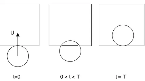
Now we consider a slightly more difficult case of a spherical moving bubble entering in a cubic box (fig. 2). The bubble velocity is aligned with the z direction of a Cartesian reference frame, the axes of this frame being parallel to the sides of the box. At the initial time, the bubble is entirely outside of the box but the top of the bubble is located at the inferior face of the box (fig. 2a). At a given instant t, the height of the bubble which is inside the box h(t) is equal to Ut (fig. 2b), and the time T corresponds to the first time when the bubble is entirely inside the box (fig. 2c). We therefore have 2R = UT where U and R are the velocity and radius of the bubble respectively.

U

t=0 0 < t < T t = T

Fig. 2: A spherical bubble entering in a cubic box

The equation (1) for the bubble is given by:

( )

x,t x y

(

z Ut

)

R 0

F = 2 + 2 + − 2 − 2 = (21)

At a given time t smaller than T, the surface area of the spherical cap inside the volume V of the box is given by A(t) = 2πRh(t) = 2πRUt. Its integration gives:

T R 2 dt ) t ( A 2 T 0 = π

∫

(22)

The calculation of the LHS of (15) is slightly more difficult because one must consider separately three different zones inside the cubic volume V, corresponding to the points swept two times by the interface of the bubble during [T], the points swept a single time and the points that do not see the bubble at all, which give zero contribution to the LHS of (15). The calculation is done is the appendix. At the end we obtain:

T R 2 dv n . w 1 2 V j _j π =

∫ ∑

(23) in accordance with (22).

3. On the different forms of the Leibniz rule (or Reynolds transport theorem) for a surface

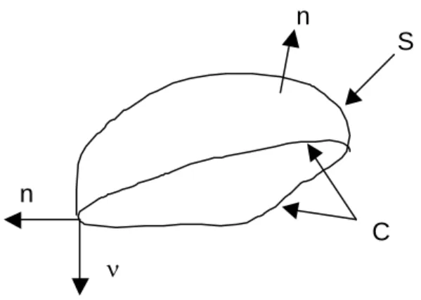
3.1. An open surface evolving freely in space

S

C n

n

ν

Fig. 3: An open surface evolving freely i n space

The boundary of the open surface S is a closed curve C. We denote by n the unit vector normal to the surface and by ν the unit vector normal to the bounding curve C, located in the plane tangent to the surface.

We can decompose the surface velocity vector w into its normal and tangential components:

( )

w.n n w w

(

I nn

)

.w

w = + t ⇔ t = − (24)

where I is the identity tensor in 3D space and I−nn is a surface projection operator which can be thought of as the identity tensor in the 2D surface (Nadim, 1996). From its definition (24), it is clear that wt is the projection of the vector w in the plane tangent to the surface. We

can calculate the surface divergence of the vector w:

( )

w.n .n .w

( )

w.n .n w . w . _{s t s s t} s =∇ + ∇ =∇ + ∇ ∇ (25)

where it should be noted that the surface divergence of the complete vector w and the one of its projection wt differ of a quantity equal to the product of the normal displacement velocity

defined by (7) and the surface divergence of n. In the particular case of the normal vector n, it should be noted that its surface divergence ∇s.n coincides with the usual spatial divergence

∇.n evaluated on the surface (Nadim, 1996) because we have:

(

I nn

)

: n I: n .n n . s = − ∇ = ∇ =∇ ∇ (26) since −nn:∇n =−n_in_jn_i,j =−n_j

(

n_in_i/2

)

_,j =0 because nini = 1.

The Leibniz rule, or Reynolds transport theorem, for a surface is given by (Aris, 1962):

( )( )

w.n .n da fw . dC f t f fda dt d C t S S

∫

∫

∫

⎟ + ν ⎠ ⎞ ⎜ ⎝ ⎛ _{+ ∇} ∂ ∂ = (27)

∫

∫

⎟ ⎠ ⎞ ⎜ ⎝ ⎛ Ψ _{+Ψ∇ −∇ Ψ} = Ψ S T S _dt .w w. .nda d da n . dt d (28)

where Ψ is a tensor field of any rank. Taking the particular case of the vector Ψ = nf, the Leibniz rule (27) is retrieved.

Making f = 1 in Eq. (27) and considering the particular case of a closed surface, the following simple result is obtained:

( )( )

∫

∫

= ∇ S Sda w.n .n da dt d (29)

3.2. A surface evolving within a fixed volume

The extension of the theorem (27) when one considers only the portion of a surface S(t) instantaneously contained in a fixed volume V (fig. 4) is not trivial. This extension has been done by Gurtin et al. (1989).

δV V S(t) C(t) n N

Fig. 4: A portion of surface i ncluded i n a fixed volume V

We denote by S(t) the portion of the surface instantaneously contained inside the fixed volume V and C(t) the intersection curve between the two surfaces S(t) and ∂V. On each point of the curve C(t), we can define simultaneously the unit vector n normal to the surface S(t) and the unit vector N normal to the boundary surface ∂V, outwardly directed. Gurtin et al. (1989) show that a portion of the derivative given by (27) must balance the outflow of f due to the transport of portions of S(t) across ∂V. The extended theorem reads:

( ) ( )

(

( )( )

)

( )

_{( )}

dC N . n 1 N . n n . w f da n . n . w f f fda dt d 2 ) t ( C t S t S − − ∇ + =

∫

∫

∫

& (30)

where f& is called the normal time derivative of f by the authors. It can be noted that the term involving wt in (27) is absent in (30) (the two terms on the bounding curve C of (27) and (30)

do not coincide and they have not the same significance) because Gurtin et al. (1989) assumed that wt = 0. When the velocity w is not normal to the surface, they give an extended version of

the theorem (30) (see their remark 3):

( ) ( )

(

)

_{( )}

dC N . n 1 N . w f da w . f f fda dt d ) t ( C 2 t S s t t S

∫

∫

∫

− − ∇ + = & (31)

but they do not give the demonstration of (31). Later, Jaric (1992) extended the result (30) to a portion of a moving surface inside a nonfixed volume and retrieved the result (30) for a fixed volume. Making f = 1 into the equation (30) gives:

( ) ( )

( )( )

( )

_{( )}

dC N . n 1 N . n n . w da n . n . w da dt d 2 ) t ( C t S t S − − ∇ =

∫

∫

∫

(32)

where the two surface integrals concern all surfaces inside V while the line integral lies over the intersections of the surfaces with the boundary ∂V.

3.3. Application to the determination of the surface area

When the global instantaneous interfacial area concentration SV is desired, it is equivalent to

determine the surface area A contained into the volume V since the two are related by (11). The time derivative of A is simply given by (32):

( )( )

( )

( )

_{( )}

dC N . n 1 N . n n . w da n . n . w dt dA 2 ) t ( C t S ∇ − ₋ =

∫

∫

(33)

The relation (33) was postulated by Lhuillier et al. (2000) and was demonstrated by Morel et al. (1999) into a slightly different (but equivalent) form. The only difference between (33) and the equation (27) in our previous paper (Morel et al., 1999) is that the expression of the first term in the RHS (Right Hand Side) of (33) was not given, this term being replaced by a general source term γ expressed per unit volume and per unit time. The difference between (33) and the equation (2) of Lhuillier et al. (2000) is that these authors added a volumetric source term γ in the RHS of (33) which was attributed to the coalescence and break-up phenomena. In fact, it can be shown that the equation (33) does not contain the coalescence and break-up phenomena, and that these phenomena should be added, as it was demonstrated by Lance (1986) on the case of dispersed flows and Junqua (2003) on the case of stratified flows.

Candel & Poinsot (1990) start from the equation (28) to derive their balance equation for the flame surface area in a single-phase reacting flow. Making Ψ = n into (28) gives:

(

nn: w .w

)

da .wda dt dA ) t ( S s ) t ( S

∫

∫

− ∇ +∇ = ∇ = (34)

( )( )

∫

∇ = Sw.n .n da dt dA (35)

and (29) is retrieved. The comparison of the equations (35) and (33) shows that the outflow term is missing in the equation derived by Candel & Poinsot (1990). This is a direct consequence of the fact that they start from the theorem (28), which is valid for a surface evolving freely in space, and not from the theorem (30) more adapted to the study of a portion of a surface included in a fixed volume V.

3.4. Illustration on several examples

3.4.1. A moving bubble entering in a cubic volume

In this paragraph, we reconsider the example of a moving bubble entering in a cubic box illustrated on fig. 2 in order to verify the relation (33) on a simple analytical case. The geometrical equation defining the bubble surface is always given by (21) and we recall that the portion of the surface instantaneously contained into the box is given by A(t) = 2πRh(t) = 2πRUt (paragraph 2.4.3), therefore we obtain:

RU 2 dt dA _{= π}

(36)

The two terms in the RHS of (33) are calculated in the appendix (Eqs. A.5-A.6), we obtain:

( )

( )∇ = π α

∫

2 t S .n w.n da 2 RUsin (37)

( )

( )

= π α − −

∫

2 2 ) t ( C dC 2 RUcos N . n 1 N . n n . w (38)

Their sum is therefore equal to 2πRU, in accordance to (36).

3.4.2. A plane surface moving in a sector

Now we verify the equation (33) on the case illustrated on fig. 1 (see paragraph 2.4.2). We recall that the problem is 2D and that the surface area instantaneously contained into the volume V of the sector is given by A(t) = Ut tan(α), therefore:

α = tanU dt

dA

(39)

As we have a plane surface in this case, the curvature term is nil and the outflow term is given by:

( )

( )

α = α α = − −

∫

Utan cos sin U dC N . n 1 N . n n . w 2 ) t ( C (40)

where n is assumed to be upwardly directed, therefore n.N is equal to zero on the left side of the volume V, where N is horizontal, and equal to – sinα on the right side (fig. 1).

4. Local transport equations for the void fraction and the interfacial area concentration

4.1. Local instantaneous transport equations

The first local instantaneous transport equation is the so-called topological equation for the phase indicator function χk given by Eq. (9). The second local instantaneous transport

equation is the one for δI which can be derived directly from (9) and (10) (Lance, 1986; Drew,

1990; Junqua, 2003) or from Eq. (33) which can be rewritten as:

( )( )

w.n .n dv

( )( )

w.n n.N da dv dt d I V V I VδI =

∫

∇ δ −

∫

δ

∫

∂ (41)

Using Green’s theorem on the last term of (41) and assuming that the volume V becomes infinitely small, Eq. (41) gives:

( )

[

w.n n

]

( )

w.n .n . t I I I +∇ δ =δ ∇ ∂ δ ∂ (42)

where it is not useful to indicate the sense of n since it appears twice in each term of (42). It can be demonstrated that (Marle, 1982):

(

Iwt

)

I s.wt

.δ =δ∇

∇ (43)

Adding (43) to (42) and taking (24) and (25) into account yields:

[ ]

w .w . t I I s I +∇ δ =δ ∇ ∂ δ ∂ (44)

Splitting ∇.(δIw) as w.∇δI + δI∇.w and taking into account that ∇s.w=

(

I−nn

)

:∇w, and

then subtracting δI∇.w from the two members of (44) yields:

w : n n . w t I I I + ∇δ =−δ ∇ ∂ δ ∂ (45)

an equation found by Lhuillier (2003).

They are many equivalent equations to represent local instantaneous transport of surfaces and (42), (44) and (45) are only three examples. The preference is to be given to (44) which looks like a traditional transport equation and bears many resemblances with the macroscopic transport equation proposed a long time ago by Ishii (1975).

4.2. Averaged transport equations

Realistic physical situations often develop very complicated interfaces, therefore a statistical treatment is necessary. Drew (1990) (see also Drew & Passman, 1999) use the ensemble

average over a set of equivalent processes. Denoting this ensemble average by < >, the average of the topological equation (9), taking (10) into account, gives:

I k k k n . w . w t =− ∇χ =+ δ ∂ α ∂ (46)

where αk = <χk> is the statistical volumetric fraction of presence of phase k, often called the

“void fraction”. One can also average the equation (42) which gives:

( )

w.n n

( )

w.n .n . t a I I I +∇ δ = δ ∇ ∂ ∂ (47)

where aI = <δI> is the statistically averaged interfacial area concentration. Drew (1990)

introduced two different averaged velocities: a scalar one and a vector one. The scalar averaged velocity is the one suggested by (46), it is defined by:

I I k I I k k a n . w n . w W = δ δ δ ≡ (48)

Hence (46) can be rewritten:

k I k W a t = ∂ α ∂ (49)

Drew (1990) called (48) the “average interfacial normal velocity”. We can see that it corresponds to the speed at which phase k expands itself by ‘eating’ the other phase. The vector averaged velocity suggested by Eq. (47) is defined by:

( )

( )

I I I I I a n n . w n n . w W = δ δ δ ≡ (50)

Denoting ∇.n by H (H is here the total curvature, which must not be confused with the mean curvature: the total curvature is twice the mean curvature), and defining the averaged total curvature by: I I I I a H n . H = δ δ ∇ δ ≡ (51)

Drew arrived at the following form for the interfacial area concentration transport equation:

(

)

( )

(

)

4 4 3 4 4 2 1 S I a I k I I I H H n . w t H W a . t a Φ − δ + ∂ α ∂ = ∇ + ∂ ∂ (52)

where Φs denotes a source term per unit area which is attributed to the coalescence and

established for spherical bubbles (Wu et al., 1998; Hibiki & Ishii, 2000a, Yao & Morel, 2004):

(

)

(

)

_⎢⎣⎡ +∇

(

_⎥⎦⎤ ∂ ∂ ⎟⎟ ⎠ ⎞ ⎜⎜ ⎝ ⎛ α π + ⎥⎦ ⎤ ⎢⎣ ⎡ _{+∇ α} ∂ α ∂ α = ∇ + ∂ ∂ G 2 I G I G I I V n . t n a 12 V . t a 3 2 V a . t a

₎

(53)

shows that it is a little bit more complicated, nevertheless a common term appears in the RHS of (52) and (53) since H=2/R=2a_I /3α for spherical bubbles with R = 3α/aI being the

Sauter mean radius of the bubbles and α corresponds to the gas phase. The quantity n in (53) is the bubble number concentration.

Now, we can also take the average of the equation (44), rather than (42), to obtain:

w . w . t a s I I I +∇ δ = δ ∇ ∂ ∂ (54)

which suggests us to introduce the following transport velocity:

I I I I I a w w V = δ δ δ ≡ (55)

It can be noted that WI and VI are equal as soon as wt = 0 can be assumed. If this is not the

case, a particular choice for wt must be made and the two transport velocities WI and VI are

different.

The general transport equation (54) and the transport equation (53) derived for bubbly flows are different. Therefore, we should verify their compatibility in the particular case of a bubbly flow. Their left-hand sides are identical as soon as the averaged velocity defined by (55) is replaced by the mean gas velocity VG which is the center of mass velocity of the bubble

swarm. It is simply assumed that for a dispersed bubbly flow, the two velocities transporting the interfacial area and the void fraction are close together, therefore VI can be simply

replaced by VG. The link between the two right-hand sides of (53) and (54) is more difficult.

Lhuillier (2004b) derived such a link in an approximated manner, under a similar assumption that the interface velocity w is close to the velocity of the phase having the minor fraction of presence. An equation similar to (54) was also obtained by Séro-Guillaume & Rimbert (2005) using a method based on volume averaging. Two different closures for the macroscopic velocity VI based on thermodynamic arguments are also proposed by these authors.

4.3. Link with the time averaging operator

In paragraph 2.3, we have defined a time-averaged interfacial area concentration given by Eq. (12). When the flow is steady, one can assume that the statistical average can be advantageously replaced by a time average (ergodicity assumption). If we make this assumption (aI is equivalent to ST for a steady flow), we obtain for the different time-averaged

∑

= ∂ α ∂ = j k k k k T n . w n . w T 1 t W S (56)

which is a well-known relation when using a time averaging operator (Ishii, 1975; Delhaye, 1981). k j k k I T n n . w n . w T 1 W S =

∑

(57)

∑

= j k I T n . w w T 1 V S (58)

∑

= j k T n . w H T 1 H S (59) with ST defined by (12).

4.4. Link with the volume averaging operator

In paragraph 2.2, we have defined a volume-averaged interfacial area concentration given by Eq. (11). When the flow is spatially homogeneous, one can assume that the statistical average can be advantageously replaced by a volume average (ergodicity assumption). If we make this assumption (aI is equivalent to SV for a homogeneous flow), we obtain for the different

volume-averaged quantities: da n . w V 1 t R W S V S k k k V =

∫

_⊂ ∂ ∂ = (60)

where Rk is the spatial volumetric fraction of phase k. The relation (60) is a well known

relation when using a volume averaging operator (Kolev, 2002). We have also:

(

w.n

)

n da V 1 W S V S k k I V =

∫

_⊂ (61) da w V 1 V S V S I V =

∫

_⊂ (62) da H V 1 H S V S V =

∫

_⊂ (63)

with SV defined by Eq. (11).

4.5. Illustration on a fixed bubble growing linearly in time

We reconsider the example of section 2.4.1. The geometrical equation defining the surface motion is given by Eq. (16). This motion is purely radial hence w.nG = W = cte. If we assume

that the statistical average can be replaced by a time-average over a time interval [0,T], we obtain <δI> = ST defined by (12). As w.n is equal to the constant radial velocity W, we obtain:

WT 1 n . w 1 T 1 S j _j T =

∑

= (64)

hence ∂ST/∂t = 0. The three averaged velocities WG, WI and VI defined by Eqs. (56)-(58) are

given by WG = W and WI = VI = WnG since wt = 0. Expressing the normal nG as in Eq. (A.4),

we obtain immediately:

(

)

(

)

_{( )}

t R W S 2 n . W S V S . W S . T G T I T I T =∇ = ∇ = ∇ (65)

and we have also:

( )

w.n .n W IH WSTH

I ∇ = δ =

δ (66)

which is identical to (65) since H=2/R.

Now we assume that the statistical average can be replaced by a spatial average over a volume V. We obtain <δI> = SV defined by (11). Therefore we have:

V RW 8 t S V R 4 S V 2 V π = ∂ ∂ ⇒ π = (67)

where we assume that the bubble surface is entirely contained within the volume V. We also have: 0 da n V W da n W V 1 V S W S V S V S I V I V = =

∫

_⊂ =

∫

_⊂ = (68)

since S is a closed surface and, for the curvature term:

( )

V RW 8 V R 4 R 2 W S R 2 W n . n . w 2 V I π = π = = ∇ δ (69) which is identical to (67).

It is important to remark that, if the transport equation (52) (without the last term since the mean curvature does not fluctuate) is verified using a time average or a volume average, the equilibrium between the different terms does not occur in the same manner. When using a time averaging operator, we obtain:

(

)

( )

and S / t 0 R W S 2 n . n . w W S . T T I I T = δ ∇ = ∂ ∂ = ∇ (70)

( )

and S W 0 V RW 8 n . n . w t S I V I V = δ ∇ = π = ∂ ∂ (71)

Hence, we see that the RHS of the transport equation is balanced by the divergence of the convective flux if we assume a steady situation and is balanced by the transient term if we assume a spatially homogeneous situation. Here the situation studied is not steady and not homogeneous, but the transient term is erased by the time averaging in the first situation and the convection term is erased by the spatial averaging in the second one. This example shows the importance of the choice of the averaging operator which is more adapted to the physical situation: steady or unsteady, homogeneous or not.

5. Transport equation for the flame surface density in a turbulent reacting flow

In single-phase reacting flows, combustion takes place on preferential zones where the different reactants are mixed together. These zones can be volumetric ones (flame pockets) or nearly surface ones (thin sheets in comparison to the other scales of the flow). In this last situation, called the flamelet regime, one can define a flame surface embedded in the 3D space of the flow. The mean reaction rate can be estimated as the product of the consumption rate per unit surface by a flame surface density. Infinitely fast, reduced or complex chemistry models are included in the modeling of the consumption rate per unit flame area. The flame surface density is the available flame area per unit volume and is analogous to the interfacial area concentration in two-phase flow.

The flame surface density, often denoted by Σ, obeys a transport equation called the Σ-equation (Candel & Poinsot, 1990; Boudier, 1992; Trouvé & Poinsot, 1994; Veynante et al., 1996; Van Kalmthout & Veynante, 1998). In what follows, we derive the exact Σ-equation from the equations presented in section 4. The derivation is made is the general case of a turbulent flow.

In the flamelet regime, the flame front reduces to a thin sheet which can be approximated as a 2D surface embedded in the 3D space occupied by the flow. The 2D surface has a velocity field w which can be decomposed into the sum of the flow velocity and the flame propagation velocity with respect to the flow (Candel & Poinsot, 1990; Trouvé & Poinsot, 1994; Peters, 1999):

n S v

w= + (72)

where v is the flow velocity and S is the flame propagation speed. We must discuss on the physical significance of Eq. (72). The flame front is assimilated to a surface separating the fresh gas side labeled as 1 from the burnt gas side labeled as 2. If we assume the continuity of the tangential component of the fluid velocity through the flame surface (vt1 = vt2), the

tangential component of the velocity w can be chosen equal to the common fluid tangential velocity (wt = vt1 = vt2). As a consequence, the two fluid velocities only differ in their normal

component: w = v1 + (w – v1).n1n1 and w = v2 + (w – v2).n2n2. Denoting S1 = (w – v1).n1 and

S2 = (w – v2).n2, we obtain w = v1 + S1n1 and w = v2 + S2n2 which are two relations like (72)

but where S, v and n depends on the side considered: fresh or burnt gases. The key is the mass jump condition across the frame front which imposes that the mass flux is conserved because the flame surface itself is assumed to have no mass. Denoting the mass flux density due to the reaction rate by m& and denoting n = n1 = -n2, we can write:

(

1

)

2

(

2

)

1 1 2 2

1 w v .n w v .n S S

m& =ρ − =ρ − =ρ =−ρ (73)

This relation shows that m& is intrinsic to the flame (it does not depend on the side) therefore we prefer use m& instead of S1,2. Using (73), the relation (72) can be rewritten as:

n m v n m v w 2 2 1 1 ρ + = ρ + = & & (74)

The starting point of the derivation of the Σ-equation is Eq. (44) which can be rewritten as:

[ ]

w

(

I nn

)

: w . t I I I +∇ δ =δ − ∇ ∂ δ ∂ (75)

Substituting (74) into (75) and taking the ensemble average yields:

(

I nn

)

: v m .n n m . v . t k s I k I k I k I ∇ ρ δ + ∇ − δ = ρ δ ∇ + δ ∇ + ∂ Σ ∂ _{& &} (76)

where Σ = <δI> is the flame surface density. We can also define δI-weighted averaged

quantities by the following relation:

Σ ψ δ = δ ψ δ ≡ ψ I I I s (77)

The flow being turbulent, one may classically decompose the flow velocity vk into a mean and

a fluctuating parts (Reynolds decomposition):

k k

k V v

v = + ′ (78)

Using (77) and (78), the equation (76) becomes:

(

)

(

)

(

)

43 42 1 & 4 4 4 3 4 4 4 2 1 4 4 4 3 4 4 4 2 1 4 4 3 4 4 2 1 & 43 42 1 43 42 1 curvature s k a s k k A k s k n propagatio flame s k transport turbulent s k transport mean k n . m v : n n v . V : n n V . n m . v . V . t T T ∇ ρ Σ + ′ ∇ − ′ ∇ Σ + ∇ − ∇ Σ = = ⎟ ⎟ ⎠ ⎞ ⎜ ⎜ ⎝ ⎛ ρ Σ ∇ + ′ Σ ∇ + Σ ∇ + ∂ Σ ∂ (79)

The equation (79) is the equation (3) of Veynante et al. (1996). The LHS of (79) contains three convection terms: convection by the mean velocity Vk, convection by the fluctuating

velocity <vk’>s and convection by the mean propagation velocity

s k

n m

ρ& . The RHS of (79) contains two terms due to the surface divergence of the flow velocity field (see Eq. (76)). These terms represent the stretch of the flame surface density Σ due to the velocity divergence

acting in the tangent plane. Due to the Reynolds decomposition, two different stretch terms appear: one due to the mean velocity field (term ATΣ) and one due to the fluctuating velocity

field (term aTΣ). The last term combines the propagation speed

k

m ρ

& _{and the total curvature}

∇.n of the surface. Typical closure relations for the Eq. (79) are proposed by Veynante et al. (1996) and Van Kalmthout & Veynante (1998). It should be noted that, if the fresh gas density is approximately equal to the burnt gas one (ρ1 = ρ2), the gas velocity v and the

propagation speed S becomes continuous through the flame surface and the relation (72) is retrieved.

We also note that the stretch due to the mean velocity field (term ATΣ) involves the orientation tensor nn _s which is the surface average of the dyadic product of the normal vector n by itself. Veynante et al. (1996) proposed algebraic closure relations to express this tensor in the case of experimentally measured flames. In the following section, transport equations for quantities like nn _s are given for the case of two-phase liquid-liquid dispersions. An equation quite similar to Eq. (79) has been postulated by Vallet et al. (2001) for the modeling of the atomization of a liquid jet into a droplet spray.

6. Introduction to the theory of anisotropic interfaces

In the preceding sections, the ensemble-averaged interfacial area concentration has been denoted by aI and the volume-averaged one by SV. In this section, we summarize results

obtained in the context of volume-averaging (e.g. Wetzel & Tucker, 1999) and others obtained in the context of ensemble-averaging (e.g. Lhuillier, 2003). At the end, we use the volume-averaging in order to numerically calculate averaged quantities like the interfacial area concentration SV. So we advertise the reader that, in order to avoid a change of notation

two times in this section, the interfacial area concentration will be denoted by SV throughout

this section.

6.1. Area tensors and their transport equations

In situations where gas-liquid interfaces become anisotropic (non spherical), the interfacial area concentration is not sufficient to describe them accurately, because this is a scalar quantity. The anisotropic surfaces exhibit a tensorial character which can be described by introducing the following area tensors (Wetzel & Tucker, 1999):

da n n V 1 ˆ A da n n V 1 ˆ A V S i j ij V S

∫

∫

⊂ ⇔ = ⊂ = (80)

for the second order tensor,

da n n n n V 1 ˆ A da n n n n V 1 ˆ A V S i j k l ijkl V S

∫

∫

⊂ ⇔ = ⊂ = (81)

for the fourth order tensor and so on… The area tensors (80) and (81) are defined onto a control volume V, as in the paper of Wetzel & Tucker (1999). When all the interfaces within this control volume are closed surfaces, only the even-order area tensors are useful, the odd-order area tensors being zero-valued. In what follows, we do not make the distinction between

a given tensor like A or its typical component Aij. Due to the fact that the normal vector n is

a unit vector, the following interesting properties of area tensors can be noted:

( )

ij V S i j ijkk V V S ii A da n n V 1 A S V A da V 1 A tr A = = = = = =

∫

∫

⊂ ⊂ (82)

In particular, the trace of the second-order area tensor is equal to the global (volume-averaged) surface area concentration SV and one can normalize an area tensor of any order by

dividing it by SV. The normalization of the second order area tensor gives the orientation

tensor nn _s introduced in section 5. One can also introduce the deviator of the area tensor:

ij V ij V S i j ij ij S 3 1 A da 3 1 n n V 1 q ⎟ = − δ ⎠ ⎞ ⎜ ⎝ ⎛ _{− δ} ≡

∫

⊂ (83)

where δij is the Kronecker symbol. The quantity (83) is called the interface anisotropy tensor

or interface tensor.

The transport equation for the second-order area tensor can be deduced from the equation (44) and the evolution equation for the normal vector n (Wetzel & Tucker, 1999; Lhuillier, 2003):

i k j jk j ji i i i n n n L n L n . w t n dt dn + − = ∇ + ∂ ∂ = (84)

where Lij is a short notation for the surface velocity gradient ∂wi/∂xj. Combining Eqs. (44)

and (84), then averaging, one obtains:

(

i j k l i j kl i k jl j k il

)

kl I I j i ij L n n n n n n n n n n n n w . t A δ − δ − δ + δ = δ ∇ + ∂ ∂ (85)

which was obtained by Lhuillier (2004a).

On the other hand, by averaging Eq. (44) or taking the trace of Eq. (85), we obtain:

(

I nn

)

:L w . t S I I V +∇ δ = δ − ∂ ∂ (86)

which is equivalent to (54). Combining Eqs. (85) and (86), the transport equation for the interface anisotropy tensor (83) is obtained:

kl il k j jl k i l k ij j i I I ij j i ij L n n n n n n 3 n n 3 n n . w t q ⎟ ⎟ ⎠ ⎞ ⎜ ⎜ ⎝ ⎛ δ − δ − ⎟⎟ ⎠ ⎞ ⎜⎜ ⎝ ⎛ δ + δ = ⎟ ⎟ ⎠ ⎞ ⎜ ⎜ ⎝ ⎛ δ ⎟⎟ ⎠ ⎞ ⎜⎜ ⎝ ⎛ δ − ∇ + ∂ ∂ (87)

In the case of liquid-liquid dispersions, interesting results have been obtained by Doi & Ohta (1991) and later by Lhuillier (2003). The original paper of Doi & Ohta (1991) was concerned with two incompressible fluids having the same viscosity and density, mixed with equal volume fractions. The assumptions of equal viscosities and equal concentrations have been suppressed in the work of Lhuillier (2003).

Lhuillier (2003) assumed that the velocity w of the interfaces is close to the translation velocity v of the dispersed phase, which itself is close to the average velocity V of the emulsion, because the two liquids have approximately the same density. In the RHS of (86), the velocity gradient Lij can be replaced by the microscopic deformation tensor dij = ½(Lij +

Lji) because of the symmetry of the tensor product ninj. This microscopic deformation tensor

is assumed to be close to the average deformation tensor <ddij> of the dispersed phase,

therefore Eq. (86) becomes:

d V V d : q S . V t S − = ∇ + ∂ ∂ (88)

where Aij has been replaced by qij because <ddii> = 0. Under the same simplifying

assumptions, Eq. (87) becomes:

d ij V d ki jk d kj ik d kl kl ij d kl l k ij j i I d ki jk d kj ik ij ij d S 3 2 d q d q d q 3 2 d n n 3 n n q q q . V t q − − − δ + ⎟⎟ ⎠ ⎞ ⎜⎜ ⎝ ⎛ δ − δ = ω + ω + ∇ + ∂ ∂ (89)

where ddij and ωdij are the symmetric and anti-symmetric parts of the tensor Lij. The equation

(88) shows that the evolution of SV is stopped whenever the tensor qij vanishes (isotropic

interfaces). The author said that (88) is not able to reproduce coalescence of droplets and proposed to add a term like – σα(1−α)G0SV2 in the RHS of (88):

(

)

2 V 0 d V V S G 1 d : q S . V t S α − σα − − = ∇ + ∂ ∂ (90)

where σ is the surface tension and α is the volumetric fraction of one of the two phases. The dependence of the coalescence term in α(1−α) allows to reduce the coalescence intensity as the flow becomes dilute (α tends to 0 or to 1). The factor G0 is a function of the volumetric

fractions and the dynamic viscosities of the two phases. It is given by:

(

)

2 1 2 2 1 2 1 1 2 2 2 2 1 0 2 / 3 G η α + η α + η η η α + η α = (91)

If the macroscopic deformation tensor <ddij> and the macroscopic rotation rate tensor <ωdij>

are known (as well as α and V), the system of the two equations (89)-(90) is not completely closed because one need to express the fourth order tensor Aijkl = <δIninjnknl>. The simpler

closure for this fourth order tensor is the one proposed by Doi & Ohta (1991). They proposed the following decoupling approximation:

kl ij V ijkl A A S 1 A = (92)

Substituting Eq. (92) into (89), one obtains:

(

ij ji

)

V ki jk kj ik kl kl ij ij kl kl V ij ij S 3 1 q q q 3 2 q q S 1 q . V t q κ + κ − κ − κ − κ δ + κ = ∇ + ∂ ∂ (93)

where κij = <ddij> + <ωdij> is the macroscopic velocity gradient. Doi & Ohta (1991) added

two relaxation terms in the RHS of Eqs. (88) and (93) to take into account the surface tension effects. The surface tension has mainly two effects: it makes the interfaces more isotropic (shape relaxation towards spherical shape) and it decreases the surface area concentration by shape relaxation and coalescence of the droplets. At the end, the system proposed by Doi & Ohta (1991) reads:

(

)

2 V V ij V ji ij V ki jk kj ik kl kl ij ij kl kl V ij S : q t S q S S 3 1 q q q 3 2 q q S 1 t q λµ − κ − = ∂ ∂ λ − κ + κ − κ − κ − κ δ + κ = ∂ ∂ (94)

where the coefficients λ and µ are given by:

(

)

(

1 2

)

1 0 2 1 c c / c / c c + = µ η σ + = λ (95)

where η0 is the dynamic viscosity common to the two phases and c1 and c2 are positive

numbers which can be functions of the volumetric fraction α. It should be remarked that the convection terms V.∇SV and V.∇qij are not included in the model (94) of Doi & Ohta (1991).

Later Lhuillier (2004a) proposed the following linear closure relation for the fourth order tensor (see also Hand, 1962):

(

)

(

ij kl ik jl il jk jk il jl ik kl ij

)

jk il jl ik kl ij V ijkl A A A A A A 7 1 35 S A δ + δ + δ + δ + δ + δ + + δ δ + δ δ + δ δ − = (96)

This relation has been established for the three-dimensional situations. In the case of two-dimensional situations, the numerical coefficients must be changed in order to guarantee that the trace of the tensor qij remains zero (Lhuillier, private communication):

(

)

(

ij kl ik jl il jk jk il jl ik kl ij

)

jk il jl ik kl ij V ijkl A A A A A A 6 1 24 S A δ + δ + δ + δ + δ + δ + + δ δ + δ δ + δ δ − = (97)

The relation (97) is linear, unlike the relation (92) which is quadratic. Therefore, it is expected that (97) will be correct for small deformations only and (92) will be more adapted for large deformations. This will be verified later (figs. 11-12).

6.3. Numerical tests of Doi-Ohta’s model in simple 2D configuration.

In order to test the model proposed by Doi & Ohta (1991), and in particular the decoupling approximation (92), simple numerical tests can be done. We restrict ourselves to 2D situations and to a single inclusion. Here we study the deformations of an initially circular interface submitted to different velocity fields.

6.3.1. The system of equations for 2D situations

In 2D situations, the surface area concentration is replaced by the ratio of the length of the curve L divided by the total area Atot of the two-phase mixture:

tot V

A L

S = (98)

If an area A is enclosed into the curve C, the volumetric fraction of the dispersed phase can be defined by the ratio:

tot

A A =

α (99)

and the Sauter mean diameter dS characterizing the single inclusion can be defined as:

L A 4 S 4 d V S = α = (100)

where the factor 4 is taken because we are in a 2D situation (cylindrical inclusion). For a circular inclusion, the diameter dS is equal to the circle diameter.

The definition of the interface anisotropy tensor (83) becomes, in 2D situations:

ij V ij ij S 2 1 A q = − δ (101)

As a consequence, the equation (87) becomes:

kl il k j jl k i l k ij j i I I ij j i ij L n n n n n n 2 n n 2 n n . w t q ⎟ ⎟ ⎠ ⎞ ⎜ ⎜ ⎝ ⎛ δ − δ − ⎟⎟ ⎠ ⎞ ⎜⎜ ⎝ ⎛ δ + δ = ⎟ ⎟ ⎠ ⎞ ⎜ ⎜ ⎝ ⎛ δ ⎟⎟ ⎠ ⎞ ⎜⎜ ⎝ ⎛ δ − ∇ + ∂ ∂ (102)

Making the same simplifying assumptions as in section 6.2, the equation (89) becomes in 2D situations: d ij V d ki jk d kj ik d kl kl ij d kl l k ij j i I d ki jk d kj ik ij ij d S d q d q d q d n n 2 n n q q q . V t q − − − δ + ⎟⎟ ⎠ ⎞ ⎜⎜ ⎝ ⎛ δ − δ = ω + ω + ∇ + ∂ ∂ (103)

and finally, the equation (93) becomes:

(

ij ji

)

V ki jk kj ik kl kl ij ij kl kl V ij ij S 2 1 q q q q q S 1 q . V t q κ + κ − κ − κ − κ δ + κ = ∇ + ∂ ∂ (104)

6.3.2. The numerical procedure for 2D situations

The numerical procedure consists in discretizing the closed curve in a set of N points (N-1 segments) given by (xi,yi) in Cartesian coordinates. Knowing the positions at the previous

time step (xin,yin), one can calculate the imposed velocity field (uin,vin) = (u(xin,yin),v(xin,yin))

and then integrate the velocity field to find the new positions of the discretisation points:

dt v y dt v y y dt u x dt u x x n i n i t t n i n i 1 n i n i n i t t n i n i 1 n i 1 n n 1 n n + ≅ + = + ≅ + =

∫

∫

+ + + + (105)

where dt = tn+1 – tn is the (constant) time step. Knowing the positions (xin+1,yin+1) at the current

time step, one can calculate the newest velocity field and so on… At each time step n, all the quantities characterizing the inclusion can be calculated. The infinitesimal displacement along the curve is given by:

n i n 1 i n i n i n 1 i n i x x , dy y y dx = ₊ − = ₊ − (106)

and its length dsin is given by Pythagoras’s theorem:

2 n i 2 n i n i dx dy ds = + (107)

Then, the two components of the normal vector can be calculated by:

n i n i n i , y n i n i n i , x dy /ds , n dx /ds n =− = (108)

From the local quantities (106)-(108), one can evaluate the following global quantities:

∑

∫

= ₌− = N 1 1 i n i C n ds ds L (109)

(

)

_∑

(

)

∑

∫

∫∫

∫∫

− = − = − = + = = ∇ = = N1 1 i n i n i n i n i 1 N 1 i n i n i , y n i n i , x n i C A A n dy x dx y 2 1 ds n y n x 2 1 ds n . x 2 1 da x . 2 1 da A (110)

for the enclosed area, where the Green theorem has been used. From (109)-(110), one can easily calculate the quantities defined by (98)-(100).

The calculation of the area tensors is simply given by:

∑

− = = N1 1 m n m n m , k n m , j n m , i tot n ... ijk n n n ...ds A 1 A (111)

and their normalized form by:

∑

− = = N1 1 m n m n m , k n m , j n m , i n ... ijk n n n ...ds L 1 Aˆ (112)

Having the second order area tensor by (111) and SV by (98), the interface anisotropy tensor

qij can be calculated using its definition (101).

6.3.3. Simple shear

In the first numerical test, we impose a simple shear for the velocity gradient: 0

v , y

u =κ = (113)

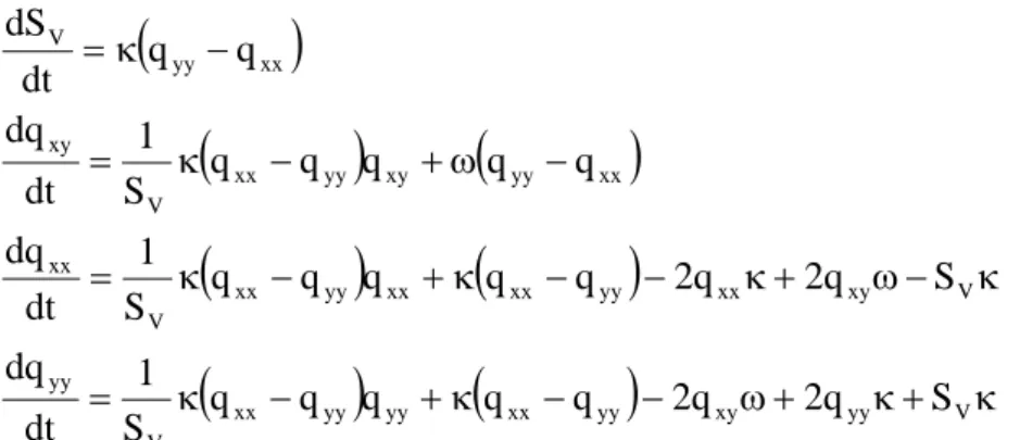
The corresponding 3D case has been studied analytically by Doi & Ohta (1991). In a 2D situation with a velocity field given by (113), it is easy to show that the system (88)-(104) degenerates in the following manner:

xy yy xy V yy xy xx xy V xx V xx 2 xy V xy xy V q q q S 1 d dq q q q S 1 d dq S 2 1 q q S 1 d dq q d dS − = γ + = γ − − = γ − = γ (114)

with γ = κt being the non-dimensional time. In this first test, we assume that the initial radius of the inclusion is equal to 1 (m), therefore giving an enclosed surface A equal to π (m2

) in a squared area Atot = 4 (m2). The void fraction α defined by (99) is therefore equal to 0.785. We

choose an arbitrary value of κ = 0.1 (s-1

) and we calculate 100 time steps with a time step value dt = 0.1 s. The final time in the calculation is therefore equal to t = 10 s and the final non dimensional time is γ = 1. The numerical curve has been discretized with 1000 points.

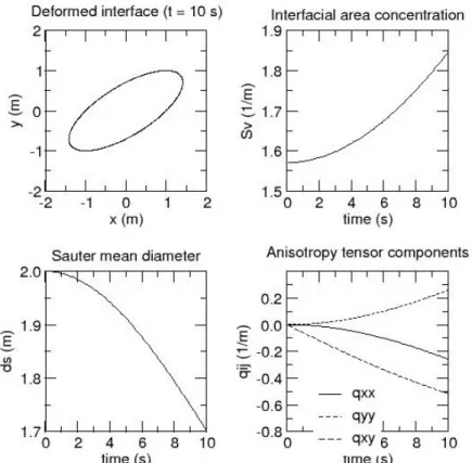
Fig. 5: Sketch of the deformed interface at the end of the calculation and time evolution of the volume-averaged quantities Sv, dS and qij (simple shear)

The deformed interface at the end of the calculation as well as the time evolution of the volume averaged quantities SV, dS and the components qij are presented on fig. 5. The stretch

of the interface by the shear velocity gradient (fig. 5a) causes an increase in the surface area concentration SV (fig. 5b). Accordingly, the Sauter mean diameter of the inclusion decreases

(fig. 5c) and the three components of the anisotropy tensor separate from zero (fig. 5d). It can be seen that the trace of the anisotropy tensor given by qxx + qyy is constantly equal to zero, as

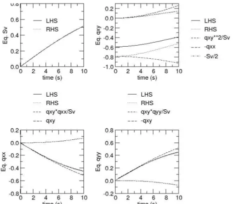
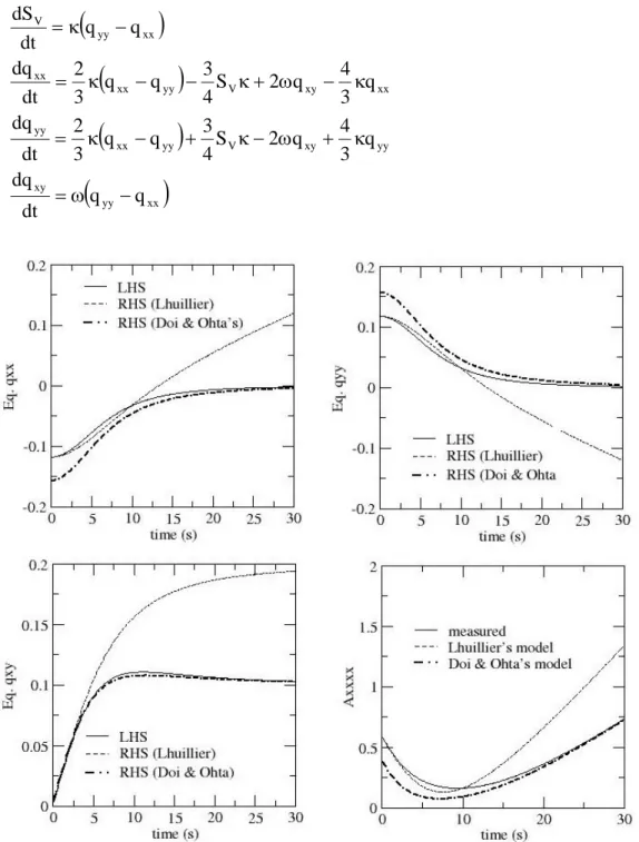
expected by the definition of the anisotropy tensor. The velocity field (113) being divergence-free, the area enclosed in the curve must be conserved, which can be verified by the invariance of the void fraction during time, constantly equal to 0.785. Now we can evaluate each term of the model equations (114) from our numerical simulation (fig. 6). In particular, the two sides of each of these equations can be compared. It can be seen that, except for the component qxy, all the equations (114) are perfectly balanced.

Fig. 6: Comparison of the LHS and RHS of the model equations (114) together with the different contributions in their RHS (simple shear)

This discrepancy between the two sides of the qxy equation should be attributed to the

decoupling approximation (92), because the model equations (114) are based on this decoupling approximation, and our numerical simulation is not. This is confirmed by the comparison of the fourth order tensor Aijkl and its approximated value AijAkl/SV (Eq. 92). The

comparison of the four components Axxxx, Axxxy, Axxyy and Axyyy calculated from the

simulation with their approximated values Axx2/SV, AxxAxy/SV… is illustrated on fig. 7. It can

be seen that the components Axxxy and Axyyy are quite well predicted by (92) but that Axxxx and

Fig. 7: Test of the decoupling approximation (92) on the four components Axxxx, Axxxy,

Axxyy and Axyyy of the fourth order area tensor (simple shear)

6.3.4. Uni-axial elongation and rotation

In the second numerical test, the initially circular inclusion is submitted to the following velocity field: y x v , y x u =κ +ω =−ω −κ (115)

The velocity field (115) is also divergence-free. It corresponds to the addition of an uni-axial elongation (u = κx, v = -κy) and a rigid body rotation characterized by an angular velocity ω (u = ωy, v = -ωx). The velocity gradient tensor κij, the deformation rate tensor Dij and the

rotation rate tensor Ωij are given by:

⎟⎟ ⎠ ⎞ ⎜⎜ ⎝ ⎛ ω − ω = Ω ⎟⎟ ⎠ ⎞ ⎜⎜ ⎝ ⎛ κ − κ = ⎟⎟ ⎠ ⎞ ⎜⎜ ⎝ ⎛ κ − ω − ω κ = κ 0 0 , 0 0 D , (116)

(

)

(

)

(

)

(

)

(

)

(

−

)

+κ

(

−

)

− ω+ κ+ κ κ = κ − ω + κ − − κ + − κ = − ω + − κ = − κ = V yy xy yy xx yy yy xx V yy V xy xx yy xx xx yy xx V xx xx yy xy yy xx V xy xx yy V S q 2 q 2 q q q q q S 1 dt dq S q 2 q 2 q q q q q S 1 dt dq q q q q q S 1 dt dq q q dt dS (117)

We submit the same initially circular interface to the velocity field given by (115) with the values κ = ω = 0.1 s-1

. The time simulated is equal to 30 s. The same quantities as before are illustrated of the figs. 8-10. It can be seen that, at the time t = 30 s, the interface is strongly deformed (fig. 8a). The figure 9 shows that the equations (117) for SV and qxy are rapidly

balanced and that the two other equations for qxx and qyy are balanced later. Similarly, the

figure 10 shows that the decoupling approximation gives quite good results for the two components Axxxy and Axyyy as soon as the beginning of the deformation. The two other

components Axxxx and Axxyy tend more slowly to their approximated values and attain them at

the end of the deformation. Therefore, it can be said that the decoupling approximation (92) is better for strongly anisotropic interfaces.

Fig. 8: Sketch of the deformed interface at the end of the calculation and time evolution of the volume-averaged quantities Sv, dS and qij (elongation and rotation)

Fig. 9: Comparison of the LHS and RHS of the model equations (117) (elongation and rotation)

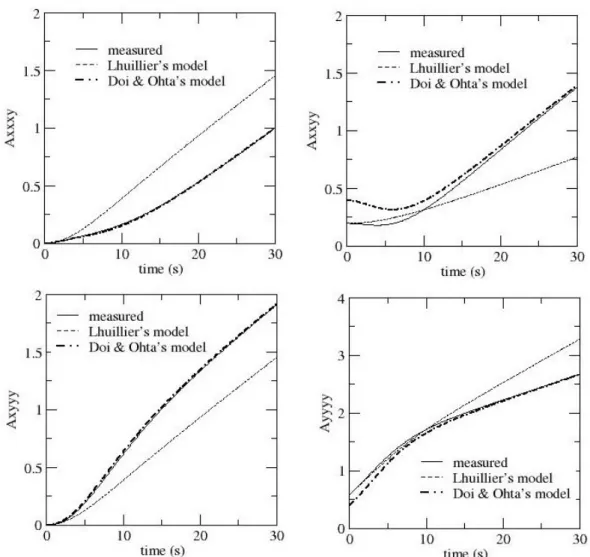
Fig. 10: Test of the decoupling approximation (92) on the four components Axxxx, Axxxy,

We have also compared Lhuillier’s model (Lhuillier, 2004a) in his two-dimensional version (Eq. 97) to the decoupling approximation (92) proposed by Doi & Ohta on the case illustrated on fig. 8 (elongation and rotation). Substituting the closure relation (97) into the equation (103) and applying it to the velocity field (115) (together with the SV equation) gives the

following set of modeled equations:

(

)

(

)

(

)

(

yy xx

)

xy yy xy V yy xx yy xx xy V yy xx xx xx yy V q q dt dq q 3 4 q 2 S 4 3 q q 3 2 dt dq q 3 4 q 2 S 4 3 q q 3 2 dt dq q q dt dS − ω = κ + ω − κ + − κ = κ − ω + κ − − κ = − κ = (118)

Fig. 11: Comparison of Lhuillier’s model (97) to the model (92) on the elongation and rotation case. Comparison of the LHS and RHS of the model equations (118) for the quantities qxx, qxy and qyy. Comparison of the measured and modeled quantity Axxxx.

Fig. 12: Comparison of Lhuillier’s model (97) to the model (92) on the elongation and rotation case. Fourth order tensor components Axxxy to Ayyyy.

The equilibrium of the SV transport equation visible on fig. 9a has not changed because the SV

equation (118)1 does not depend on the closure used for Aijkl and hence is the same as (117)1.

The results of this comparison are illustrated on figures 11 and 12. It can be seen that Lhuillier’s model is more efficient at the beginning of the calculation, hence in the slight deformations case, unlike Doi & Ohta’s model which gives better results at the end of the calculation, hence when the deformations are large. The remaining challenge is to find an interpolation between the two models (92) for big deformations and (97) for small deformations. This issue is left for future work.

7. Conclusion

This paper deals with surface transport equations in two-phase and single-phase reacting flows. The problem of the determination of the flame surface density in single-phase reacting flows is quite similar to the determination of the interfacial area concentration in two-phase flows. We have summarized the theoretical foundations of these two problems, and shown the connection between them. The different definitions of a volumetric surface area by spatial, temporal and ensemble averages have been recalled. The different forms of the transport equation for such a quantity are derived and it should be remarked that it is a consequence of the Leibniz rule, or Reynolds transport theorem, for a portion of a surface evolving in a fixed

volume. We have also derived the flame surface density transport equation in a turbulent reacting flow from an equation previously derived for the interfaces in two-phase flows, showing the mathematical connection between these two problems. As the interfacial area concentration is a scalar quantity, it cannot deal with anisotropic interfaces which exhibit a tensorial character. The mathematical tools which are necessary to study the anisotropic interfaces are presented in section 6, and the example of the system closure in the case of laminar incompressible liquid-liquid dispersions is given (Doi & Ohta, 1991; Lhuillier, 2004a). At the end, we have tested these two models on simple 2D numerical simulations of the deformation of a single inclusion in an imposed velocity field. The 2D version of the transport equations are derived and their results are compared to the simulation results. Two different velocity fields are imposed: a simple shear and a velocity field composed of an elongation and a rotation. This kind of simulations gives a simple mean to test different approximations for the fourth order area tensor, which is the key issue when using a system composed of the interfacial area transport equation and the anisotropy tensor transport equation. We have found that the decoupling approximation (92) proposed by Doi & Ohta (1991) works better when the interfacial anisotropy is important, unlike Lhuillier’s model which is better for small anisotropy.

Acknowledgements: The author is fully indebted for the fruitful discussions on the subject with Profs. Jean-Marc Delhaye, Daniel Lhuillier, Michel Lance, Jean Fabre, and Dr. Alexandra Junqua. We also thank the French Commissariat à l’Energie Atomique, Electricité de France, AREVA NP and the French Institute for Nuclear Safety for their financial support in the context of the NEPTUNE project.

APPENDIX

A moving bubble entering in a cubic volume

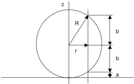
In paragraph 2.4.3., we study the case of a moving bubble entering in a cubic volume (fig. 2). The difficulty is to calculate the LHS of the Eq. (15). To do this, we must consider separately three different zones inside the cubic volume V, corresponding to the points swept two times by the interface of the bubble during [T], the points swept a single time and the points that do not see the bubble at all, which give zero contribution to the LHS of (15). We illustrate this on figure A which illustrates the position of the bubble with respect to the inferior face of the box at the end of the process (t = T).

r R

a b b

Fig. A: A bubble enteri ng i n a box (t = T) z

We use the cylindrical coordinates system (r,φ,z), r being the horizontal distance to the symmetry axis (fig. A). Using Pythagoras’s theorem, it is easy to verify that the distances a and b indicated on the figure are given by a =R− R2 −r2 and b= R2 −r2 . A point in the box located at an altitude z smaller than a has been swept by two interfaces during the time interval [0,T], the normal velocity of these two interfaces being given by:

2 2 r R R U n . w =± − (A.1)

where the + sign corresponds to the top interface of the bubble, and the – sign corresponds to the bottom interface. The result (A.1) is obtained by applying (7) to the equation (21), taking into account that we are on the bubble surface. A point located at an altitude z comprised between a and a + 2b only sees the first interface during [T], the displacement velocity being given by (A.1) with the + sign. A point located at an altitude z greater than a + 2b does not see any interface during [T] and therefore gives no contribution. At the end, the LHS of Eq. (15) writes: dr dzd r r R U R dr dzd r r R U R 2 dv n . w 1 R 0 2 0 r R R r R R 2 2 R 0 2 0 r R R 0 2 2 V j _j 2 2 2 2 2 2 φ − + φ − =

∫ ∫ ∫

∫ ∫ ∫

∫ ∑

π −+ −− π − − (A.2)

Each of the two integrals in the RHS of (A.2) gives 2πR3

/U. Their sum is therefore equal to 4πR3_{/U which, by virtue of the fact that 2R = UT, is also 2πR}2

T, the result given in (23). Now we will calculate the two terms in the RHS of (33). The total curvature can be calculated by the divergence of the normal vector n, which gives:

R 2 n . =

∇ (A.3)

where we have used the fact that the normal vector n has the following components:

(

x y

)

/R R n , R / y n , R / x n_x = _y = _z =± 2 − 2 + 2 (A.4)

on the surface. The angle α being measured between the normal n onto the intersection curve C and the vertical direction z, the portion of the surface which is included in the box at time t is limited by 0 < φ < 2π and 0 < θ < α where φ and θ are the surface coordinates (fig. B).

z

n α

r

N

Fig. B: Definition of the α angle

The curvature term in the RHS of (33) is therefore given by:

( )

( )

(

)

α π = θ θ θ − π = θ θ φ θ + φ θ − π = θ θ − φ = ∇

∫

∫

∫

∫

∫

α α α π 2 0 2 0 2 2 2 2 2 2 2 0 2 2 2 0 t S sin UR 2 d sin sin 1 UR 4 d sin sin sin cos sin R R U 4 d sin R r R R U d R 2 da n . n . w (A.5)

For the outflow term, it should be noted that the intersection curve between S and ∂V is a circle and that the unit vector N normal to ∂V is equal to – ez where ez is the unit vector in the

vertical direction z (fig. B). Therefore n.N is equal to – nz and the outflow term is calculated

as:

( )

( )

= − − φ= π

(

−

)

= π α − −

_∫

_∫

2π 2 2 2 0 2 z z 2 2 2 ) t ( C _R R r 2 URcos U 2 rd n 1 n r R R U dC N . n 1 N . n n . w (A.6)