HAL Id: halshs-02895908
https://hal.archives-ouvertes.fr/halshs-02895908v2
Preprint submitted on 15 Mar 2021
HAL is a multi-disciplinary open access archive for the deposit and dissemination of sci-entific research documents, whether they are pub-lished or not. The documents may come from teaching and research institutions in France or abroad, or from public or private research centers.
L’archive ouverte pluridisciplinaire HAL, est destinée au dépôt et à la diffusion de documents scientifiques de niveau recherche, publiés ou non, émanant des établissements d’enseignement et de recherche français ou étrangers, des laboratoires publics ou privés.
A Poorly Understood Disease? The Impact of
COVID-19 on the Income Gradient in Mortality over
the Course of the Pandemic
Paul Brandily, Clément Brébion, Simon Briole, Laura Khoury
To cite this version:
Paul Brandily, Clément Brébion, Simon Briole, Laura Khoury. A Poorly Understood Disease? The Impact of COVID-19 on the Income Gradient in Mortality over the Course of the Pandemic. 2021. �halshs-02895908v2�
WORKING PAPER N° 2020 – 44
A Poorly Understood Disease? The Impact of COVID-19 on the
Income Gradient in Mortality over the Course of the Pandemic
Paul Brandily
Clément Brébion
Simon Briole
Laura Khoury
JEL Codes: I14; I18; R00
Keywords: COVID-19 ; poverty; mortality inequality; labor market; housing
conditions.
A Poorly Understood Disease? The Impact of COVID-19 on the Income
Gradient in Mortality over the Course of the Pandemic
∗Paul Brandily† Cl´ement Br´ebion‡ Simon Briole§ Laura Khoury¶ First version: July 2020
This version: March 2021
Abstract
Mortality inequalities remain substantial in many countries, and large shocks such as pandemics could amplify them further. The unequal distribution of COVID-19 confirmed cases suggests that this is the case. Yet, evidence on the causal effect of the epidemic on mortality inequalities remains scarce. In this paper, we exploit exhaustive municipality-level data in France, one of the most severely hit country in the world, to identify a negative relationship between income and excess mortality within urban areas, that persists over COVID-19 waves. Over the year 2020, the poorest municipalities experienced a 30% higher increase in excess mortality. Our analyses can rule out the contribution of policy responses (such as lockdown) in this heterogeneous impact. Finally, we show that both labour-market exposure and housing conditions are major determinants of the direct effect of the epidemic on mortality inequalities, but that their respective role depends on the state of the epidemic.
JEL classification: I14; I18; R00
Keywords: COVID-19 ; poverty; mortality inequality; labor market; housing conditions
∗Declarations of interest: none.
†Paris School of Economics, France. paul.brandily@psemail.eu ‡Copenhagen Business School, Denmark. cbr.msc@cbs.dk
§Paris School of Economics & J-PAL Europe, France. simon.briole@psemail.eu ¶Norwegian School of Economics, Norway. laura.khoury@nhh.no
1
Introduction
Despite an unprecedented worldwide decline in mortality over the last century, a substantial income gradient still persists within most countries (Case et al., 2002; Cutler et al., 2006; Chetty et al., 2016;
Currie et al., 2020). These structural inequalities result primarily from individual differences between
the rich and the poor in health behaviours, information, economic or social stress (Butikofer et al., 2021) and from ecological factors, like the living environment or public health institutions (Chetty et al.,
2016; LeClere et al., 1997; Robert, 1999; Pickett and Pearl, 2001). However, sudden exogenous events
like pandemics can also significantly affect these inequalities. Historical studies have shown that past epidemics had unequal effects on the mortality of different socio-economic groups, either because they revealed latent inequalities in individual health capital or because they spread differently across living environments (Snowden,2019;Alfani,2021;Beach et al.,2021).
The COVID-19 crisis epitomizes such massive mortality shock, on a worldwide scale. In 2020, about 100 million people have tested positive for COVID-19 – among which 2.2% died – with a large number of infections and deaths also remaining undetected.1 Assessing the causal impact of this pandemic on mor-tality inequalities is therefore key, not only to inform public policy in the context of the crisis, but also to study the role of pandemics in shaping mortality inequalities from a historical perspective. However, while a growing literature has pointed out that most vulnerable socioeconomic groups were more often affected in the early months of the pandemic, most of the existing evidence remains essentially correlational.
A first challenge in measuring the causal impact of the epidemic on mortality inequality consists in isolating the specific contribution of COVID-19. Even in the absence of the pandemic, the structural health inequalities in terms of income could potentially explain the correlation between mortality and income in 2020. Disentangling between the direct effect of the pandemic and that of the policy responses (such as lockdown) represents a second important challenge which has been disregarded by the literature. Finally, a third challenge relates to the dynamics of the pandemic: many studies are based on early and short-term measures. It is unclear whether these results only reflect harvesting effects due to a temporary mortality shock on individuals particularly at risk. In particular, one cannot exclude that the income gradient gradually disappears, or is even reversed, as time goes by and the disease spreads.
In this paper, we address these challenges in the context of France, one of the most severely hit country in the world. Using exhaustive administrative data sets, we are able to study the links between income and the 2020-specific excess mortality at a very local level, for the entire country and over a long
time period. We combine daily death records of all-cause mortality provided by the French National Statistical Institute (INSEE) for the three entire years 2018-2020 with information on the municipality of residency, a very detailed geographic scale (1,600 inhabitants and 15 sq.km per municipality, on average). Leveraging the precision of our data, we study what happens, on average, between municipalities within urban areas exposed to COVID-19. Working at such a fine geographic scale allows to account for local interactions between individuals that are central to the development of health inequalities (LeClere et al.,
1997;Robert,1999;Pickett and Pearl,2001), and all the more so in the case of an epidemic.2
There are three main results in this paper. First, we confirm the existence and persistence of an income gradient in the 49,495 excess deaths that occurred in French urban areas over the two distinct waves of the epidemic (in Spring and late Fall 2020). Within a given urban area, and once population size and age are controlled for, the difference in excess mortality rates between the poorest municipalities (bottom quartile of the income distribution) and the richer ones equals 2.6 (deaths per 10k. inhabitants), i.e. 30% of the excess mortality in the non-poor municipalities in 2020. We show that the gradient uncovered during the first wave is not compensated during the second wave, but rather reappears with regularity every time the epidemic returns, so that it is the strongest in areas that got most affected by COVID-19 in 2020. Second, we propose a decomposition of COVID-19 total impact into a direct component – from COVID-19 infections – and an indirect component (e.g. mental-health consequences of lockdown policies, increased domestic violence, road accidents avoided because of the lockdown, etc. (Banerjee et al., 2020; Belot
et al.,2020;Caul,2020;Mulligan,2021;McIntyre and Lee,2020;Bullinger et al.,2020)). We rule out the
existence of a significant income gradient in the indirect component. Third, examining mechanisms, we show that labor-market exposure and housing conditions are important determinants of the variation in COVID-19 mortality and largely explain the income gradient.
This article makes several contributions to the literature on the income gradient in the specific case of COVID-19. Many papers have shown that the first wave affected more strongly deprived neighborhoods and individuals based on confirmed cases (Chen and Krieger,2021;Abedi et al.,2020;Ashraf,2020;Kim
and Bostwick, 2020; Williamson et al.,2020; Drefahl et al., 2020; Jung et al., 2020; Caul, 2020).3 Our
data allows to improve on the measurement of the specific contribution of COVID-19 to health inequality
2
Individual characteristics affecting one’s likelihood of infection also affect infection risks of others living or working nearby. Note that we introduce in our models urban-area fixed effects, so that we absorb specific local factors that may foster or hinder the spread of the epidemic (e.g. public transportation) and are unlikely to be independent from municipalities’ income.
3A few exceptions should be mentioned. Comparing US counties, Brown and Ravallion (2020),Desmet and Wacziarg (2020) andKnittel and Ozaltun (2020) find no association between median income or poverty rates and COVID-confirmed deaths. Jung et al.(2020) finds a positive relation between poverty rates and confirmed deaths in counties with a low density but rather a U-shaped relation in dense areas. According to Sa(2020), the positive association between socioeconomic deprivation and confirmed COVID deaths in the UK turns negative once self-declared health quality is taken into account.
in two ways. First, confirmed cases underestimate the number of deaths attributable to the pandemic. In particular, they do not account for false negatives or deaths on which no test has been carried out, either because testing material was lacking in hospital or simply because they occurred at home. Unre-ported cases are highly unlikely to be independent of income and may therefore bias the results of the literature based on confirmed cases. To avoid such bias, we favour all-cause mortality to confirmed cases in our estimations. Second, our approach allows to better account for the structural income heterogene-ity in mortalheterogene-ity that is found absent COVID-19. Many articles have previously documented mortalheterogene-ity inequalities between socio-economic groups and it could then be the case that the income heterogeneity in COVID-19 confirmed deaths only reflect these. In particular, in the US, where most of the evidence on the income gradient comes from, these structural inequalities may be particularly strong since the access to health care is very unevenly distributed among the population.4 We therefore use all-cause excess mortality as our main dependent variable, defined as the deviation in 2020 all-cause mortality with respect to a counterfactual (pre-COVID) period – namely the average of all-cause mortality in 2019 and 2018.5
To our knowledge, very few articles have worked on all-cause excess mortality, and all of them focused on the first wave (Calder´on-Larra˜naga et al., 2020; Krieger et al.,2020;Decoster et al.,2020). By using two successive waves in France, our paper adds to this literature by evaluating the evolution of the income gradient over time. Our analysis reveals that the relationship between income and COVID-19 mortality applies with regularity to each wave of the epidemic and that the mortality differential created does not disappear over time.6 The epidemic caused an increase in differential mortality between rich and poor municipalities that is not a simple one-time shock or anticipation effect in the deaths of the most vulnerable but is rather deepening after each wave.
This article is also the only one to disentangle between the direct and indirect effects of COVID-19 infections on mortality. Beyond the direct effect of COVID-COVID-19 infections, the epidemic could have an indirect impact that is is non-orthogonal to households’ income (e.g. mental-health consequences of lockdown policies, increased domestic violence, road accidents avoided because of the lockdown, etc.
(Banerjee et al.,2020;Caul,2020;Mulligan,2021;McIntyre and Lee,2020;Bullinger et al.,2020;
Calderon-4
By contrast, measuring the income gradient in a country like France is informative on the unequal impact of COVID-19 despite a rather equal access to health care. Comparing the income gradients found in both countries is interesting to the extent that France and the US systematically rank at both ends of the distribution of OECD countries in terms of equality of access to health care (source, see alsoCurrie et al.(2020) for a comparison of mortality trends in the US and in France.) 5Two exceptions to the literature using confirmed cases should be mentioned: Caul (2020) describes both confirmed cases and all-cause mortality – but with no counterfactual;Chen and Krieger(2021) use a counterfactual but do not consider all-cause mortality.
6
More specifically, a surplus of 1.18 (resp. 1.08) excess deaths per 10k. inhabitants is found in the bottom income quartile in the first wave (resp. second wave), as compared to richer municipalities.
Anyosa and Kaufman, 2021) and may thereby drive part of the income gradient found in the early literature.7 We exploit the quasi-natural experiment provided by the first lockdown to disentangle between both dimensions. Its uniform implementation over the territory froze the epidemic at very different stages of development. In zones with a low level of infection at the start of the lockdown, the propagation of the virus was stopped before it could have a significant impact on mortality. By contrast, in the high-infection zone, the virus had already circulated enough to have a large impact on mortality, despite the lockdown. We find no income gradient in the within-urban-area mortality in the low-infection zone, suggesting that the overall income gradient is entirely driven by the direct effect of COVID-19 infections.8
Finally, our paper speaks to the literature on the mechanisms underlying the relationship between income and COVID-19 mortality. Previous papers have highlighted the importance of labor-market exposure or housing conditions (including the first version of this paper, as of July 2020, as well as
Almagro and Orane-Hutchinson (2020); Almagro et al. (2020); Glaeser et al. (2020); Naticchioni et al.
(2020)). Building on exhaustive administrative data, we confirm the previously uncovered role of increased exposure inside and outside the house.9 We extend the aforementioned literature by examining the dynamics of the mechanisms effect under different policies and by trying to quantify the respective weight of each mechanism in explaining the variation in COVID-19 mortality.10 The impact of the share of workers with frequent social contact at work decreases in magnitude during the second wave, suggesting that employers have adjusted the management of the occupational risk over time. Housing conditions also matter less during the second wave, as the lockdown was less stringent. A horse race performed between variables related to occupational exposure and housing conditions indicates that our variables – and especially the share of essential workers and of overcrowding housing – almost fully explain the income gradient in COVID-19 related mortality.
The remainder of the paper is organized as follows: section 2 describes the data and the construction of our outcome variable, while section 3 explains the context. In section 4, we present the first evidence of an income gradient in COVID-19 mortality in France that persists across waves. In section 5, we
7
According toMulligan(2021), about 12% of March-to-October excess mortality in the US was due to non-COVID causes (a large part being the result of ”deaths of despair”).
8
We treat the low-infection zone in the West and South of France as a control group: any income gradient in excess mortality found on this group during the first wave is considered as a measure of the differentiated impact (between poor and non-poor municipalities) of the indirect effects of COVID-19 (including the lockdown). Reassuringly for our estimation strategy, we find an income gradient in this zone during the second wave.
9Further mechanisms may also include: greater levels of air pollution in poorer areas (Cole et al.,2020; Persico and
Johnson,2020), lower levels of compliance to lockdown and to self-protection measures among low-income individuals Papa-george et al.(2020), more comorbidities among poor households (Wiemers et al.,2020;Raifman and Raifman,2020) among others. While population density is also an often debated mechanism, we do not treat it as a potential mechanism given its non-significant correlation with poverty in our data.
10
Almagro et al.(2020) also examine the dynamics of the effect of labor-market exposure and housing conditions in New York City but over a shorter time period and under a different institutional context.
disentangle between the indirect and the direct effects of COVID-19 on excess mortality. Given these results, section 6 explores potential mechanisms and section 7 concludes.
2
Data and measurement
Data sources
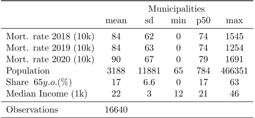
In this paper, we gather various individual-level data sets that we match using municipality-level identifiers. In France, municipalities are very small administrative units of 1,600 inhabitants and 15.3 sq.km on average; there are about 35,000 of them in 2020. Our analysis compares municipalities within urban areas. Urban areas are groups of neighboring municipalities, defined by the French National Statistical Institute (INSEE) on the basis of commuting patterns. We consider 16,640 municipalities distributed across 621 urban areas, each being made of 27 municipalities and hosting 85,000 inhabitants on average.11 The majority of our sources are exhaustive administrative data sets made available by INSEE. We provide more details on all data in appendix A1.
Measuring the impact of the epidemic on mortality
Most previous works studying the unequal impact of the pandemic are based on COVID-19 confirmed cases (infection or death). These measures suffer from several conceptual limitations.12 First, the total impact of an epidemic on mortality is a function of both the direct effects of infections (Dd), and the
indirect effects of public policies taken as a response to infections (Di). The latter relates to social changes
caused by the epidemic, such as (i) physical, psychological, and social effects of distancing13(ii) economic changes (Banerjee et al. (2020)). Furthermore, Dd can be broken down into reported infection-caused
deaths (Dd,r), unreported infection-caused deaths (Dd,u), and deaths due to altered access to health
services (Dd,a).14 Studies based on confirmed cases not only ignore the indirect effects of the epidemic
but can also suffer from severe biases arising from the salience of unreported cases and the saturation of health services.
A growing literature confirms that measures based on COVID-19 reported cases actually include significant biases. First, testing capacities and strategies have proven to vary substantially over space and time, not only across countries but even across regions or neighbourhoods (Kung et al.,2020;Rivera et al.,
11
Due to our within urban area approach, we exclude smallest urban areas made of only one municipality from the analysis. TablesB1andB2provide more descriptive statistics on our sample at the urban area and the municipality level, respectively.
12
SeeB¨ottcher et al.(2021) for a detailed discussion on this topic. 13
For instance, evidence suggests that the lockdown have reduced the transmission of the seasonal flu and of norovirus (Kraay et al.,2020).
14
2020;Borjas, 2020;Balmford et al., 2020; Silverman et al., 2020;Yorifuji et al., 2021; Wu et al.,2021). France is no exception to this rule: it ranked among the worst OECD countries in number of tests per inhabitant in May 2020 (Scarpetta et al.,2020;Foucart and Horel,2020). Another source of bias comes from the non-random testing of the population in a context of a shortage in testing resources. Typically, tests are more often conducted on symptomatic persons, the elderly or socio-economic vulnerable people, leading to overestimation of infection rates (Beaney et al., 2020; B¨ottcher et al., 2021). Finally, some individuals who die from COVID-19 are not accurately identified, due to difficulties in attributing the cause of death. This may particularly bias the number of reported cases in France, where no system was able to report the COVID-19 mortality at home (Fouillet et al.,2020).
A second limitation of analyses using only measures based on COVID-19 confirmed cases is that they ignore counterfactual mortality. To conclude about an income gradient from COVID-19 observed death actually presumes that such gradient would not exist absent the epidemic. In other words, it fails to take into account structural health inequalities between socio-economic groups. Such inequalities have been consistently documented in a wide range of countries (Case et al., 2002; Cutler et al., 2006; Adler and
Rehkopf,2008;Cutler et al., 2012; Currie and Schwandt,2016;Mackenbach et al., 2019) and have been
recently highlighted in the case of France, where the richest 5% men (resp. women) have a life expectancy of 13 (resp. 8) years longer than the poorest 5% on average over the 2012-2016 period (Blanpain,2018).15 As a consequence, accounting for the baseline inequality in mortality between rich and poor (in the absence of COVID-19) is key to accurately identify the specific contribution of the epidemic on inequality in mortality.
To address these issues, we build measures of all-cause excess mortality at the municipality level based on daily counts of deaths from INSEE. For every single individual who died in France in 2018, 2019 or 2020, this data set provides the municipality and place of death (hospital or clinic, home, care home, etc.) as well as a set of individual-level characteristics such as sex, date of birth and municipality of residency.16 Such data makes it possible to compare the mortality for the residents of a given municipality, during a given period in 2020, to the mortality in the same municipality during the same period in the two previous
15We also find such inequalities in our data in 2018 and 2019 (see Section5.1). 16
In the emergency of the COVID-crisis, INSEE made the data set available at a high frequency rate: this has induced potential measurement errors although INSEE applies corrections at each iteration. However municipalities have about one week to inform INSEE about new death. As the version of the data that we are currently using got updated on February 5, 2021, our measures should be accurate. For a discussion on the quality of the data, see theinformation provided by INSEE.
years,17 before the COVID-19 outbreak. For each municipality m, we therefore define excess mortality
during period p as follows:
Dmp = N p,2020 m − [0.5 × (Nmp,2018+ Nmp,2019)] P opulation2014 m (1)
where Nmp,y is the number of deaths of residents of municipality m during period p of year y and
P opulationm,2014is the total number of inhabitants (/10,000) of municipality m, as recorded in 2014, the
most recent available year in our data.
Using all-cause excess mortality allows us to study the impact of the COVID-19 epidemic on mortality based on a measure that is of constant quality over space and time and that is available at a fine level for a very large territory. We are therefore able to avoid the usual biases found in the literature that are due to testing or death reporting issues. Furthermore, our counterfactual analysis also allows us to take into account the structural inequalities between rich and poor in terms of mortality in order to accurately identify the impact of the epidemic on these inequalities. Finally, our measure allows us to account for both the direct and the indirect effects of the epidemic, the latter being generally ignored in the literature studying the unequal impact of the epidemic. However, one may also be interested in isolating the direct effects of the epidemic on mortality inequalities. In section 5, we develop a triple-difference strategy based on a quasi-experimental setting, which exploits natural variations in infection rates over the French territory at a very early stage of the epidemic to net out the indirect effects of the epidemic caused by the policy response. This strategy allows us to isolate the direct effect of COVID-19 infections and to study how it is distributed based on a reliable and unbiased measure of mortality.
A municipality-level analysis
The main goal of this paper is to estimate the impact of the COVID-19 epidemic on inequalities in mortality. Our approach at the municipal level allows us to study this issue from a geographical point of view, at a fine local level, and to estimate the average effect of living in a poor area on COVID-19 related mortality.18 Another - and complementary - research question relates to the estimation of the individual effect of being poor on COVID-19 mortality (i.e. the individual income gradient), for which an analysis at the individual level would be better suited. Such an analysis has the disadvantage of ignoring the role of local factors as well as that of interactions between individuals living or working in the same geographical
17We use the average of years 2018 and 2019 because taking several years makes our measure less sensitive to random events occurring in a given year. For data availability reasons, we cannot go further back in time, since death data before 2018 do not include, at the moment, information on the municipality of residency.
18Currie and Schwandt(2016) take a similar approach to study the link between poverty and mortality from a historical perspective.
area – which are known to influence the income gradient in life expectancy in normal times (Chetty et al., 2016). Given the nature of an epidemic, it is clear that individual characteristics affecting the likelihood of infection of one individual - such as poverty - will also affect the likelihood of infection of others living or working nearby. Conducting the analysis at the municipality level therefore allows us to account for local interactions between individuals and for the spillovers on COVID-19 infection probability (and related mortality) resulting from these interactions.19
3
COVID-19 in France: context and background
3.1 The temporal dynamics of the epidemic in 2020
Overall in 2020, there was 49,495 deaths in excess in French urban areas in comparison with the average of 2018 and 2019. Figure 1 represents the distribution across months of these extra deaths in France in 2020 (black line). It clearly appears that, as in many European countries, excess deaths in 2020 essentially occurred over two distinct waves that peaked in April (15,479 deaths) and November (12,537 deaths), respectively. In the remainder of this paper, we will refer to the “first wave” as the period covering March and April 2020; and the “second wave” as the period October to December 2020. In both cases, the French Government reacted by taking extraordinary containment measures. As COVID-19 first spread in the country in early 2020, the government decided of a national lockdown on March 17 and that eventually lasted until May 11. This first lockdown was the most stringent and seems to have reduced the impact of COVID-19 drastically. All workers stayed home except if their activity was deemed essential for the country and visits to elderly care homes (hereafter EHPADs) were forbidden. After a lull in the summer, the epidemic developed again until a second lockdown was decided on October 30 and continued until December 15. This second lockdown was less stringent however: (i) on top of essential private industries, factories, firms from the construction sector as well as most public services remained open; (ii) to the exception of universities most schools kept on receiving students; (iii) visits to EHPADs were allowed; (iv) parks and gardens remained open. The second lockdown got also repealed quicker, with the end of a first phase after a month when all shops opened again. Based on Google mobility data (Google LLC, 2021), Figure B1 (black line) provides evidence that the increase in time
19To the best of our knowledge, the only study able to look differentially at the individual vs the local relationship between poverty and COVID-19 mortality is the one byDecoster et al.(2020), who exploit mortality data from the first wave of the epidemic (March-May) in Belgium. Their results point to a much larger gradient at the municipal than at the individual level, confirming the existence of strong spillovers and/or local factors at the municipal level.
spent at home is much higher when a lockdown policy is in place, and more so during the first lockdown than the second.
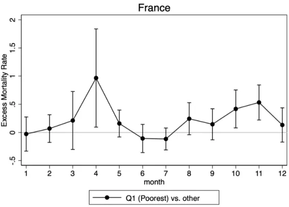
Figure 1: Monthly counts of excess deaths in French urban areas
NOTE: The figure represents the difference between the monthly number of deaths in 2020 and its average over 2019 and 2018 in the relevant zone. The “red” zone corresponds to the areas that were the most severely hit by the first wave, and that are located in the North-Eastern quarter of the country. This zone covers about 44% of the urban population of (mainland) France. The “green” zone encompasses the rest of the French territory.
3.2 Spatial heterogeneity in excess deaths
An important feature of the French case is that the spread of the epidemic was still very uneven across the country when the first lockdown was implemented (March 17, 2020). While the North-East was severely hit, the West and the South were then almost spared by the epidemic. In the remainder of this paper we call the former region the “red zone” and the latter the “green zone”. Figure 1 exhibits this spatial heterogeneity in excess deaths during the first wave. We reproduce the death toll separately for the North-East (red line) and the rest of the country (green line), the former indicating regions where COVID-19 was highly active when the first lockdown started. As is clear in the Figure, the first wave
represents 44% of the total urban population. By contrast, the green zone suffered a much smaller increase in mortality over the same period.20
Figure1thus summarizes the spatio-temporal dynamics of the COVID-19 epidemic in France in 2020. We distinguish four phases, 1: January and February are marked by a relatively low mortality in all regions of France.21 2: March and April represent the “first wave” that mostly hit the North-Eastern quarter (red zone) of the country. 3: May to September, mortality is close to normal. 4: October to December, a second wave hit the country, this time more homogeneously across the territory.
As shown in appendix Tables B3 and B4, the red zone contains less urban areas than the green zone (191 vs. 430) but these are bigger on average (39 municipalities and 12,000 inhabitants vs 22 municipalities and 6,800 inhabitants) and have more deprived municipalities (25% vs. 20%). Breaking down these statistics at the municipality level reveals however that cities in both zone are not so dissimilar. The median mortality rates in 2018 and 2019 (72 vs. 75) are very similar, and so are the share of elderly (16% vs. 17%) and median income (22,000 vs. 21,000 euros).
4
The impact of COVID-19 on the income gradient in mortality
This section highlights a key heterogeneity in all-cause excess mortality in France that appears con-sistently over the two waves: an income gradient in the total impact of the COVID-19 epidemic on mortality.
4.1 A first stylized fact
In 2020, poorest municipalities in France suffered from a greater increase in mortality, as compared to other municipalities. This stylized fact appears very clearly in Figure 2, which displays the (non-parametric) monthly cumulative number of excess deaths (per 10K. inhabitants) in 2020, separately for the poorest municipalities and other municipalities.22
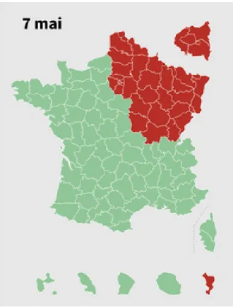
To categorize a municipality as poor, we first rank all municipalities according to the median income of their inhabitants and we define as “poor” all the municipalities that fall into the first quartile (Q1) of this distribution (cf. A1andA2for details and data). We weight each municipality by its total population
20
The classification between green and red zones follows a map issued by the Government at the end of the first lockdown (on May 7) that we detail in AppendixA2. The map is defined at the d´epartement level. A d´epartement is an administrative unit in France that encompasses on average 363 municipalities and 645,000 inhabitants. There is a total of 101 d´epartements in France. TablesB3andB4detail the total number of urban areas, municipalities, and inhabitants in each zone.
21The seasonal flu was particularly strong in 2018. 22
The cumulative number of excess deaths in month m corresponds to our excess mortality variable computed over the period from January to the month m.
in order to give an equal weight to each individual. The municipalities included in Q1 therefore represent the 25% of the French urban population living in the municipalities with the lowest median income.
Figure 2: Cumulative excess mortality rate per 10,000 inh. by poverty status
NOTE: The graph plots the cumulative sum of all excess deaths per 10,000 inhabitants from January 2020 for poor and non-poor municipalities. Poor is defined as belonging to the bottom quartile of the national distribution of municipal median income weighted by the municipality size.
Figure 2shows no specific pattern in the cumulative excess mortality rate in the first three months of 2020 (phase 1, in section3.1), followed by a marked increase from April (phase 2), that further grows as the second wave takes place (phase 4). By the end of 2020, there was, on average, 11.4 more deaths per 10K. inhabitants than usual in the poorest municipalities in France, against 8.7 in richer municipalities. In the following paragraphs, we employ an econometric approach to check whether this stylized fact holds after accounting for the influence of age and local factors.
4.2 Empirical approach
We check that the descriptive evidence displayed in Figure 2holds parametrically and test its robust-ness. We contrast the evolution of excess mortality in poor municipalities with that of richer municipalities
over the whole French territory, taking a synthetic year (the average of 2018 and 2019) as the baseline. Our main model thus writes as:
D[m,ua]p = β.Q1[m,ua]+ X[m,ua]p .Λ + γua+ ν[m,ua]p (2)
Where m indicates the municipality, ua an urban area and p a given period of the calendar year. Dp[m,ua]represents municipalities’ excess mortality rate as defined in section2(i.e. as the deviation to the average 2018 and 2019 mortality rate of the same municipality over the same period p). In our analysis, every municipality m belongs to one single urban area ua, and we therefore drop this redundant subscript in subsequent models. Xm,ua is a vector of controls including the total population size and the share of
the population above 65 years old. Importantly, we introduce γua, an urban-area fixed effect so that we
only exploit differences between municipalities located within a contiguous urban environment. This is an important aspect of our model since it absorbs specific local factors that may foster or hinder the spread of the epidemic (e.g. public transportation) and are unlikely to be independent from municipalities’ income. Our results are thus based on comparisons at a very fine spatial level. Municipalities are weighted by their total population. Standard errors are clustered at the urban-area level.
The coefficient of interest is β. It estimates the difference in excess mortality rate between munic-ipalities from the poorest (Q1) and the other quartiles (comparison group). This model identifies the heterogeneity in the causal (total) effect of the pandemic on excess mortality under the sole hypothe-sis that, absent COVID-19 and the associated public policies, the average difference in the evolution of mortality over period p (2020 vs. before) between rich and poor municipalities of the same urban area would have remained stable. Below, we use falsification tests to provide evidence that this assumption is sensible.
4.3 Results
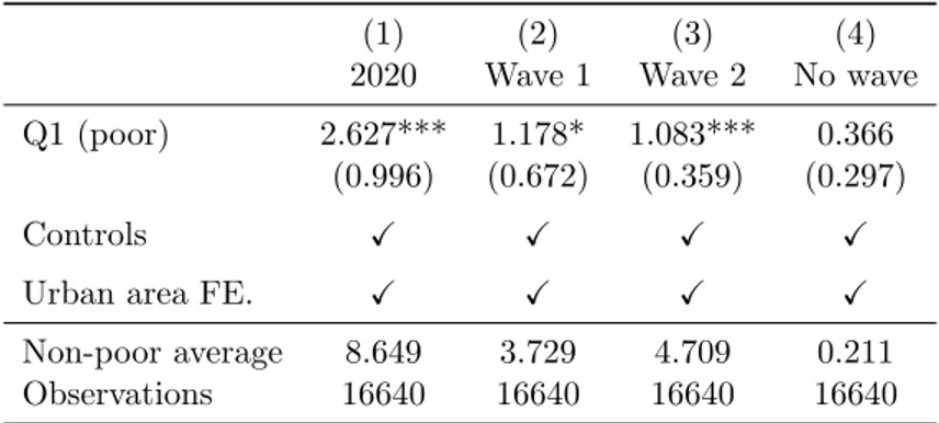
Table1reports the estimates associated to equation2. Column 1 is estimated on all urban areas from mainland France and using the cumulative excess mortality rate over 2020 as a dependent variable. On average, within a given urban area, and once population size and age are controlled for, municipalities of the poorest quartile had an excess mortality rate of 2.627 (deaths per 10k. inhabitants) higher than other municipalities. This has to be compared with the baseline average of 8.649 across municipalities of the other quartiles.
We next consider three sub-periods for 2020 that correspond to the dynamics of the epidemic described in section 3.1. In column (2) we report the coefficients associated with equation 2when considering only the first wave, that is for March and April (i.e. p = (3, 4)), while in column (3) we consider the second wave, from October to December (i.e. p = (10, 11, 12)). The income gradient is significant in both waves and slightly higher than 1 extra dead per 10,000 inhabitants. By contrast, we observe no gradient when we focus on excess mortality outside of the two waves. In column (4), we consider a synthetic period made of all the months in 2020 that we did not classify in either wave. In these months, mortality was really close to baseline (i.e. 0 excess death).
Table 1: Excess mortality rate by municipality income
(1) (2) (3) (4)
2020 Wave 1 Wave 2 No wave
Q1 (poor) 2.627*** 1.178* 1.083*** 0.366
(0.996) (0.672) (0.359) (0.297)
Controls X X X X
Urban area FE. X X X X
Non-poor average 8.649 3.729 4.709 0.211
Observations 16640 16640 16640 16640
* p<0.05, ** p<0.01, *** p<0.001. Standard errors in parentheses clustered at the urban-area level.
NOTE: This table reports the coefficients associated with equation 2. The independent variable, excess mortality rate, is computed considering four dif-ferent time periods: the whole year (column 1), wave 1 (March to April, column 2), wave 2 (October to December, column 3) and other months in 2020 outside the two waves (January, February and from May to September, column 4). By construction, column 1 is the sum of column 2 to 4. The non-poor average line reports the mean of the dependant variable in non-non-poor municipalities. Controls include total population size and the share of the population over 65 years old.
We then further decompose the effect and estimate the model for each of the 12 months separately. Figure 3plots the estimated β coefficients. The difference in monthly all-cause excess mortality between municipalities of the poorest quartile and richer municipalities closely follows the dynamics of the epidemic depicted in Figure 1 and the β only differs from 0 at the peak of the first and second waves. In other words, in each epidemic wave, mortality increases on average (Figure 1) but even more so in the poorest municipalities (Figure3).23
23
It is also important to note that the standard errors are much greater in the first wave than in any other month. This is because the excess mortality only occurred in some part of the country, as explained in section3.2, an heterogeneity we discuss at length in section5.
Taken together, these results support the idea that the income gradient we estimate for the whole 2020 year actually reflects the causal (total) effect of COVID-19 on mortality inequalities. They also provide evidence that this causal effect appears with regularity in each wave of the epidemic. We provide clearer and more detailed evidence on this last finding in section4.4.
Figure 3: Monthly difference in all-cause excess mortality by income
NOTE: The graph plots the point estimate and the 95% confidence intervals of the estimation of β from equation2evaluated each month. It accounts for the monthly difference in all-cause excess mortality between the poor municipalities and the rest, where poor is defined as belonging to the bottom quartile of the national distribution of municipal median income weighted by the municipality size.
About the definition of poverty
Our main model compares municipalities from the poorest quartile (Q1) to the others. This approach has the advantage of simplicity: by discretizing income into a simple “poor” vs. “non-poor” comparison, it greatly reduces the dimension of the problem and allows the exploration of heterogeneity and mechanisms in the following sections below. In appendix C1 we explain this definition carefully. In particular, we show that contrasting the evolution of mortality in each of the four quartiles leads to a clear monotonic pattern. That is (within an urban area) the increase in excess mortality (during COVID-19 waves)
de-creases in municipalities’ income. This monotonicity is robust to a number of alternative partitioning of the distribution. And, given this monotonic income gradient, pooling non-poor municipalities together to form a comparison group actually attenuates the differences in mortality rates we estimate (as Q1 is closer to the Q2-Q4 average).
Robustness
The presence of a stronger increase in mortality of the poorest municipalities is robust to a number of alternative specifications. We only summarize these results here; comprehensive analysis can be found in AppendixC. As already mentioned, we test alternative grouping of municipalities into distinct quartiles, deciles, and halves of the income distribution (cf. appendix C1). The result also holds when excluding elderly care homes. These were severely hit during the epidemic and one may worry that their location could drive a spurious correlation between municipality-level income and mortality. Removing all death records in such institutions does not alter our conclusion (cf. Table C3). Next, we compute the income gradient separately for different age categories (FigureC3): the income gradient increases with age, except for the category of people over 85 years old, who may represent a particularly vulnerable population irrespective of the level of income. In other words, except for the very old, the size of the gradient increases with the size of the death toll.
Finally, we run an additional falsification test which compares mortality in 2019 and 2020 to the same baseline of 2018. Reassuringly, we find a gradient in 2020 excess mortality but none in 2019 excess mortality (see appendix C2.2).24
4.4 Urban Area analysis
Figure 3 suggests that there is a proportional link between the income gradient and excess mortality at the country level. We directly test this hypothesis at a much finer geographical level, namely the urban-area level. To do so, we first estimate the gradient for each month of 2020, separately for each of the 421 urban areas that include both poor and non-poor municipalities. We then regress this measure on the total excess mortality of the urban area in the same month (see Appendix D for more details). This exercise yields a clear message: an increase in the urban area excess mortality rate by one (death per 10k. inhabitant) is associated with an increase of the gradient of a bit more than 0.3 (more death per
24Given that we only have 2018 as a reference period for this test, our main falsification test compares excess mortality over the whole year so that our comparisons are not polluted by potential seasonal shocks. However, note also that none of the monthly coefficient of 2019 (v.s. 2018) is significant at the 5% level (cf. FigureC2).
10k. inhabitant) (cf. Table D1). That is, an increase in the total intensity of an epidemic wave at the urban area level will disproportionately affect poor municipalities of this urban area.
Immediately related is the question of the evolution of the urban-area level gradient over the two waves. Two hypotheses are compatible with current evidence of a gradient: first, it could be that poor areas are hit first and non-poor areas subsequently catch-up; second, it could be that poor areas are structurally more exposed to COVID-19. For the first time, our data allows to test these two hypotheses over a one-year and two-wave span. To perform such test, we simply consider the 243 (among 421) urban areas that suffered positive excess mortality in each of the two waves.25 We find that, in these urban areas, the average income gradient in both wave is positive (cf. Table D2). This means that, in these urban areas, although residents of poorer municipalities suffered more in the first wave, they also did so in the second wave. In other word, over a one year period, we find no evidence of catch-up of the richer municipalities.
This longer-term perspective provide new evidence on the impact of COVID-19 on mortality inequal-ities: it shows that the income gradient identified in the first wave is a regular feature of the pandemic that is not compensated later in 2020.
5
Direct and indirect effects of the COVID-19 epidemic: evidence
from a quasi-natural experiment
The previous section has established evidence of an income-related heterogeneity in the total impact of the pandemic on mortality in France. This income gradient can result from both the direct and indirect effects of COVID-19. According toMulligan (2021), about 12% of March-to-October excess mortality in the US was due to non-COVID causes (a large part being the result of ”deaths of despair”). A recent literature has documented that these indirect deaths due to economic and social changes related to the epidemic - including lockdown policies - have disproportionately affected the poor.26 In this section, we take advantage of the quasi-natural experiment induced by the first lockdown to clear these potential indirect channels.
25
These represent 72% (96%) of urban areas (population) in the red zone and 43% (69%) in the green zone. 26
According toMcIntyre and Lee(2020), unemployment in time of lockdown is expected to have a strong impact on suicide rates – and we know that poor individuals are more likely to have jobs that cannot be done remotely and were therefore more often laid off during the lockdown (Gottlieb et al., 2021;Palomino et al.,2020). Bullinger et al.(2020) have shown that stay-at-home orders increase domestic violence in poor households but not in households with above-median income. The strong variation in car crashes and in pollution levels due to the lockdown could also differently affect municipalities depending on their income (Brodeur et al.,2021). Drug overdose and alcohol abuse could also be the source of larger deaths of despair during the lockdown in poor areas.
5.1 Identification strategy
At the core of our strategy is the fact that the first lockdown was implemented uniformly over the country while the epidemic was at very heterogeneous stages of development across regions. In particular, based on an external classification provided by the government on May 7, we can distinguish regions strongly hit by the epidemic as early as mid-march (the red zone), from regions where the epidemic was at a much earlier stage of development when the first lockdown was decided (the green zone). Although this classification was only provided towards the end of the first lockdown, we indeed show in Appendix E that it strongly correlates with indicators of the spread of COVID-19 before lockdown. Importantly for what follows, we also show in this appendix that the sharp heterogeneity in the spread of the virus between the two zones in mid-March is largely unrelated to socio-economic factors potentially affecting inequalities in mortality between rich and poor municipalities and that excess mortality in both areas was very similar in 2019 (compared to 2018) and in early 2020 (compared to 2018 and 2019).
This quasi-experimental setting provides a unique opportunity to compare the evolution of excess mor-tality in two areas equally affected by lockdown restrictions27 and sharing similar characteristics (health care system, other institutions, etc.) but unequally exposed to COVID-19. Our setting is comparing within-urban areas gradient. Our claim is that the evolution of the within-urban-area gradient would have been comparable (on average between green and red areas) absent COVID-19 and the associated public policies. In other words, we assume that the probability for an urban area to be exposed to COVID-19 is independent of the evolution of its poor vs. non-poor mortality differential that would have occurred absent COVID.
To disentangle the direct effects of COVID-19 on excess mortality from its indirect effects, we treat the green zone as a control group: we consider the income gradient in excess mortality found in this zone during wave 1 as a measure of the differentiated indirect impact (between poor and non-poor municipalities) of COVID-19. By contrast, the income gradient found in the red zone captures both the direct and the indirect effects of the epidemic. The difference between the two estimated gradients can thus be attributed to the direct impact of COVID-19.28 In a sense, this approach is very similar to a triple-difference strategy where the triple-difference across zones (first triple-difference) in the wave-1-specific evolution
27FigureB1(AppendixB) supports the idea of a very uniform enforcement of the lockdown policy, since the increase in time spent at home compared to normal conditions is very similar across zones.
28
As mentioned in section 2, we define the indirect impact as deaths caused by public policies taken as a response to the epidemic and related socio-economic changes, as opposed to the direct impact which captures those directly related to COVID-19 infections (deaths + hospital congestion). Given that the epidemic was not totally absent from the green zone during the first wave, such approximation introduces errors that attenuate the magnitude of the direct effects and their corresponding income gradient.
(second difference) of the mortality gradient (third difference) identifies the causal direct effect of the epidemic on poor municipalities’ mortality rate. We assume here that, on average, within-urban-area difference between poor and non-poor municipalities in the indirect impact of COVID-19 on mortality is similar between the red and the green zones. Note that this is much less demanding than assuming that the indirect impact of the epidemic is the same across both zones.
5.2 Income gradient and the direct impact of COVID-19
Double-differences by zone
We first re-estimate Equation 2 for each zone in each month and we plot the coefficients of interest on Figure 4 (the zone-specific equivalent of Figure 3). It clearly appears that no gradient is found in the green zone during the first wave, unlike in the red zone and despite common lockdown restrictions. This leads us to conclude that there is no income gradient in the effect of such policies - that we defined as the indirect effect of the epidemic - on excess mortality. By contrast, the Figure shows a marked income gradient in excess mortality whenever the level of infection is high (i.e. wave 1 in the red zone; wave 2 in both zones). This suggests that the income gradient is only to be found in the direct effect of COVID-19 infections.
Figure 4: Excess mortality by income and zone
NOTE: The graph plots the point estimate and the 95% confidence intervals of the estimation of β from equation 2 evaluated each month on each zone separately. It accounts for the monthly difference in all-cause excess mortality between the poor municipalities and the rest in each zone, where poor is defined as belonging to the bottom quartile of the national distribution of municipal median income weighted by the municipality size. The red zone corresponds to the areas that were the most severely hit by the first wave, and that are located in the North-Eastern quarter of the country. This zone covers about 44% of the urban population of (mainland) France. The green zone encompasses the rest of the French territory.
A triple-difference strategy
To test more formally the existence of an income gradient in the direct effect of the epidemic, we exploit the quasi-natural experiment provided by the first lockdown by employing a triple-difference strategy that adds the red vs. green dimension (defined at the d´epartement level) to the double-difference setting used in section 4. Formally, we estimate the following model:
D[m,d]p = β.Q1m+ δ.Redd+ ρ.Redd.Q1m+ X[m,d]p .Λ + γua+ νmp (3)
The main coefficient of interest ρ estimates the difference between red and green zones in the within urban-area difference between rich and poor municipalities’ excess mortality. Xm,d represents a vector
of controls and γua the full set of urban-area fixed effects,29 both defined as in Equation 2. ρ measures
the causal effect of the pandemic cleared of national public policies (including the lockdown) on excess mortality under the sole hypothesis that, absent COVID-19 infections, the average difference in the evolution of mortality in a given month (2020 v.s. 2019 and 2018) between rich and poor municipalities of the same urban area would have been the same in red and green zones. Standard errors are clustered at the d´epartement level, the most aggregated level of treatment status in this setting.30
In this setting the period of interest is that of March and April (first wave), and estimating Equation 3both before the pandemic broke (January and February) and between waves (May-September) provides several tests of our identification assumption. Furthermore, evaluating the equation during the second wave (October-December), when no clear difference in mortality between the two zones stood out, ensures that both zones are comparable. All monthly coefficients are reported in Figure 5. Consistent with our hypothesis, the Figure shows no significant difference in excess mortality between zones outside of the first wave. This difference first increases in March, due to the early direct effects of the epidemic, but remains insignificant at a 5% level. Conversely, in April, at the peak of wave 1, the main coefficient is strongly significant and is even stronger than in the double difference.
29
Note that these urban-area fixed effects account for the risk that: (i) coincidentally, the differences in COVID-19 infection intensity across urban areas at a given point in time could be non-orthogonal to their income level; (ii) people may adapt their behaviour to the local level of infection which would bias our results (Almagro et al.,2020).
Figure 5: Income gradient in the direct effect of COVID-19 on mortality
NOTE: The graph plots the point estimate and the 95% confidence intervals of the estimation of ρ from equation3evaluated each month. It accounts for the monthly difference in all-cause excess mortality between the poor municipalities and the rest in the red and in green zones, where poor is defined as belonging to the bottom quartile of the national distribution of municipal median income weighted by the municipality size.
Robustness
In Appendix F, we take advantage of the panel nature of our data to estimate a full triple-difference strategy using death toll as the main dependent variable. It allows us to include municipality fixed effects to control for any time-invariant factor that could influence mortality at the municipality level. The nature of the result remains: over March-April, mortality increased in 2020, more so in red than in green areas, and more so in poor than non-poor municipalities. This confirms that the most severely hit municipalities are those belonging to the poorest quartile and to the red zone. Results based on the triple-difference strategy are still robust to the exclusion of elderly care homes.31
6
Potential mechanisms
In this section, we explore the role of two potential mechanisms that could explain inequalities in COVID-19 related mortality: labor-market exposure and housing conditions.32 We first describe how we measure these dimensions and confirm that each of our measure is positively correlated with poverty (section6.1). We then investigate their independent effect on COVID-19 related mortality by exploring the association between each of these measures and excess mortality as well as the dynamics of these associations across the different stages of the epidemic (section6.2). Finally, we try to quantify the extent to which these mechanisms explain the income gradient in COVID-19 related mortality and to understand which of the two prevails (section6.3).
6.1 Housing and labor-market conditions: measurement and relation with poverty
Highly-exposed occupations are successively defined as occupations with frequent direct contact with the public in usual (pre-COVID-19) business conditions, and as occupations in sectors which kept oper-ating during lockdown periods (the so-called essential workers). Informed by administrative data on the occupational distribution in each municipality, we compute (i) the worker-weighted average frequency of contact (hereafter “index of frequent contact”) and (ii) the share of essential workers, in every munici-palities. Regarding housing conditions, we use census data at the household level to measure the share of overcrowded housing units in the municipality. This variable improves on some previous measures of household size used in the literature (Almagro and Orane-Hutchinson, 2020) since it is a function of household size, dwelling size and number of rooms. At the interaction between labor-market and housing dimensions, we finally compute the share of municipalities’ households that gather at least one member aged 65 or more and one member from a younger generation who is currently employed. This measure requires occupation information from the Census, which is only available for municipalities with at least 2,000 inhabitants. We provide more details on the construction of these measures in Appendix A2 and reference the sources in AppendixA1. TableB5(AppendixB) shows descriptive statistics on the different mechanism variables.
Table G1 (AppendixB) shows the strength of the link between poverty and our (normalized) labor-market and housing measures, once included our baseline controls and urban-area fixed effects.
Munic-32We consider these two channels informed by the current literature about how COVID-19 is transmitted (Almagro and
Orane-Hutchinson,2020;Almagro et al.,2020;Glaeser et al.,2020), and given their likely positive association with poverty. We of course acknowledge that these are only two potential mechanisms among many and that we notably ignore the role of comorbidities known to be related with poverty and that most likely played a role in the observed phenomenon (Wiemers et al.,2020;Raifman and Raifman,2020).
ipalities of the poorest quartile have more occupations in contact with the public (column 1) and more essential workers (column 2). A one standard-deviation increase in the share of essential workers (respec-tively in the index of frequent contact) makes the probability to fall in the bottom quartile of the national weighted income distribution increase by 16pp (respectively 14pp). The association is even stronger with the housing-crowding variable (column 3): a one standard-deviation increase in the share of over-crowded housing amounts to a 29pp rise in the probability to be living in a poor municipality. Finally, poorest municipalities are also more likely to have multigenerational households (column 4), although the reduced sample size of municipalities with more than 2,000 inhabitants decreases the precision.33
6.2 The effect of labor-market exposure and housing conditions on excess mortality
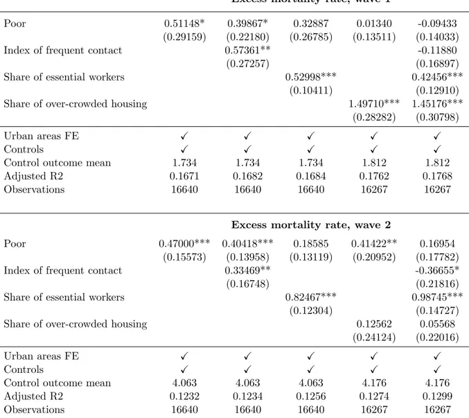
We now estimate the double-difference model exposed in Equation 2 but substituting (normalized) labor-market and housing-related measures in place of the poverty indicator. Table 2 reports the main coefficient of interest of the mechanism variables (i.e. the β of Equation 2) for each wave separately.
We first examine results for the first wave (March-April) in the upper part of Table 2: both labor-market indices and housing overcrowding exhibit significant effects. A one standard-deviation increase in the share of frequent-contact jobs leads to a rise of 0.69 deaths per 10K inhabitants on average in wave one, relative to an average level of 3.97. The respective figure for the share of essential workers is of the same order of magnitude: 0.65 units (+16%). The effect of overcrowded housing is even larger: increasing its share by one standard deviation increases excess mortality by 1.51 deaths per 10K inhabitants during the first wave (i.e. a 38% increase relative to the average excess mortality in wave one).34 In Table2, we
observe that households including both elderly and employed individuals seem to foster the transmission of COVID-19 and its associated mortality. Although the coefficient is not significant in wave one,35living
in a municipality with a one standard-deviation higher share of multigenerational households significantly increases excess mortality by 0.53 deaths per 10K inhabitants in wave two (i.e. a 10.5% increase relative to the average excess mortality).
33
The coefficient indicates that a one standard-deviation increase in the share of multigenerational households increases the probability to be in the poorest quartile by 7pp, but the p − value is only equal to 0.175.
34
Interestingly, we find a small positive but non-significant effect of municipal density on excess mortality rate. However, the link with poverty is not significant, and we therefore do not include density in our mechanism variables. For a deeper analysis of density, seeGerritse(2020). In contrast, the effect of over-crowded housing on excess mortality is five times as large. Consistent withAlmagro and Orane-Hutchinson(2020);Allain-Dupr´e et al.(2020), it means that the density in the municipality matters less than the density at home to explain differences in COVID-19 related mortality.
35
The sample on which this effect is estimated is restricted to municipalities with more than 2,000 inhabitants. We reproduced our results for our main three variables on that reduced sample. All the point estimates are of the same magnitude as the ones shown in table 2, although standard errors are larger due to the smaller sample size. Results are
Table 2: Effect of mechanism variables on COVID-19 related mortality
Index of frequent contact Share of essential workers Share of over-crowded housing Multigenerational hh Excess mortality rate, wave 1
Main coefficient 0.69281* 0.64594*** 1.51233*** 0.30218
(0.35777) (0.14160) (0.30694) (0.42948)
Urban areas FE X X X X
Controls X X X X
Control outcome mean 3.971 3.971 4.001 4.480
Adjusted R2 0.1673 0.1679 0.1762 0.3161
Observations 16640 16640 16267 3989
Excess mortality rate, wave 2
Main coefficient 0.45774** 0.88799*** 0.40256** 0.52526***
(0.19625) (0.12777) (0.17475) (0.16278)
Urban areas FE X X X X
Controls X X X X
Control outcome mean 5.089 5.089 5.127 5.020
Adjusted R2 0.1228 0.1256 0.1268 0.2298
Observations 16640 16640 16267 3989
* p<0.05, ** p<0.01, *** p<0.001. Standard errors in parentheses are clustered at the urban-area level.
This table shows the result of regressing municipalities’ excess mortality rate in each wave on mechanism variables measuring either housing conditions or occupational exposure. The upper part of the table shows results for the first wave (March-April) while the bottom part of the table shows results for the second wave (October-December) on municipalities in all urban areas. Each column reports the result of a separate regression examining one mechanism. The main coefficient corresponds to the effect of the mechanism variable on the excess mortality rate. The mechanism variables have been normalized such that coefficients can be interpreted in terms of the effect of a one standard-deviation change, and can be compared with each other. All regressions include urban areas fixed-effects and control for total population and for the share of inhabitants over 65 y.o. in the municipality. The outcome-mean line reports the mean of the excess mortality rate per 10K inhabitants in each wave.
Our data allows us to measure the dynamics of the housing crowding and occupational exposure in different contexts over the year 2020. FiguresG1toG4(AppendixG) complement Table2by showing the monthly effect of each normalized mechanism variable on the normalized excess mortality rate, including population controls and urban-area fixed effects. Reassuringly, none of our mechanism variables has a significant effect on excess mortality outside of the two waves of the pandemic.36 Their impact is quite comparable across both waves, except for the effect of the share of over-crowded housing which decreases in magnitude during the second wave, consistent with the less strict implementation of the lockdown policy (see section3 for more details). We can also compare the coefficients found at the beginning and the end of each wave, where March and October capture mortality before the implementation of the lock-down, and April and November-December measure mortality under the lockdown.37 While the effect of frequent social contacts remains constant throughout each wave, the coefficients on the share of essential
36
Except for one coefficient out of the 48 tested, which is the share of over-crowded housing in July.
37Because of an approximate two-week lag between infection and mortality, November only partly captures the effect of the second lockdown. We also define the end of the second wave as December only, and it does not affect the results.
workers and the share of over-crowded housing significantly increase from the beginning to the end of wave one.38 The growing importance of both housing conditions and the possibility of remote working is consistent with limited movement out of the house under the lockdown, except for essential workers who were the only ones to go to the workplace. We do not find this within-wave pattern, however, for wave two: indeed, although movement was more restricted in November-December, people were already spending most of their time at home in October, as remote working was already prevalent, which was not the case in March. In addition, as opposed to the first lockdown, schools remained open, which could both explain why the coefficient on over-crowded housing was higher during the first wave than during the second wave, but not at the end of the second wave compared to the beginning.39 Based onGoogle LLC(2021) data, FigureB1describes two facts that are consistent with the dynamics of the housing and labor-market exposure: (i) time spent at home is higher during the first lockdown than during the second; (ii) time spent at home is higher at the end than at the beginning of each wave, with the exception of December where it decreases again.
Previous literature has already established a link between physical contact (at home or at work) or maintained activity in the workplace during lockdown and COVID-19 exposure (Almagro and
Orane-Hutchinson,2020;Almagro et al., 2020; Naticchioni et al.,2020;Angelucci et al., 2020). We are able to
provide evidence at a fine level both geographically – since we have administrative data at the municipal level while covering the whole national territory – and sector-wise – as the definition of essential workers is at the 3-digit occupation level.40 We are also able to uncover the role of the interaction of labor-market and housing channels: workers increase their risk of catching the disease when going to the workplace, and transmit it to vulnerable persons when living in multigenerational households. Finally, we examine the dynamics of the effect over the whole year 2020 and under different lockdown conditions. Almagro and
Orane-Hutchinson(2020) andAlmagro et al.(2020) highlight a growing importance of housing crowding
over time compared with commuting in explaining COVID-19 infection, that they justify by the fact that essential workers were gradually laid off over time. The different policies implemented and the lower
38Although we do not have enough precision on the reduced sample where the effect of the share of multigenerational households is measured to draw any conclusion, we observe that the pattern on FigureG4is consistent with the evolution of the epidemic.
39Several reasons may explain the lower coefficient in December: first, there is anecdotal evidence that compliance was lower during the second lockdown. Second, if the lockdown was lifted on December 15th, shops were allowed to reopen from the end of November already, in anticipation of Christmas shopping. Moreover, people were traveling throughout France during the Christmas break, giving less importance to housing conditions in the municipality of residence.
40Almagro et al. (2020) exploit both occupation data from the American Community Survey and ZIP-code level and individual geolocation data to track time spent outside of home, but they focus on New York City only. Angelucci et al.
incidence of layoffs in France compared with the US during the pandemic may explain why we do not find a similar pattern.
6.3 Disentangling the role of each mechanism
To understand which mechanism prevails, we perform a horse race between our mechanism variables. Table3reports the results for the first wave (top panel) and the second wave (bottom panel) in all urban areas. Column (1) gives the difference in excess mortality rate between poor and non-poor municipalities. While the frequent contact variable has a minor effect on the poverty coefficient, columns (2) to (4) show that the inclusion of the share of essential workers and overcrowded housing make the coefficient of poverty shrink. In the first wave, the initial coefficient of poverty diminishes by 36% when the share of essential worker is included, and by 97% when the share of over-crowded housing is included. The last column shows that the covariates altogether absorb all of the poverty effect, which is not significant anymore, while housing conditions and the share of essential workers still play a significant role in explaining excess mortality. Similarly, in wave 2, a high share of the poverty effect is absorbed by the mechanism variables (64%), but here the share of essential workers appears as the main channel of the income gradient. It therefore confirms the previous analysis on the dynamics of the epidemic (section6.2).
It is reasonable to think that there is an overlap between the group of workers with frequent contacts in their job and essential workers (e.g. cashiers, bus drivers, etc.).41 The effect of having frequent contacts in the job drops when the essential worker variable is included during the first wave. It suggests that non-essential workers with frequent contact in normal business conditions do not suffer more from the pandemic during the first wave, since the lockdown probably prevents them from having such contacts. Conversely, being an essential worker alone increases the risk of COVID-19 related mortality, meaning that the increase in risk partly comes from commuting, in addition to social contact in the workplace. During the second wave, the inclusion of both occupational exposure variables even yields a negative coefficient on the contact variable. If we do not want to put too much emphasis on this result, one explanation could be that more protective measures have been taken for these over-exposed workers, maybe to the extent that they become more protected than the average worker.42 Essential workers, however, continue to be hit more severely by COVID-19 despite these protective measures because they are going to the workplace more frequently.
41
The correlation between both variables is 0.4. Out of the ten occupation codes with the highest index of frequent contact, six include essential workers.
42
Think for example of a shop assistant, who must constantly wear a face mask and use hydro-alcoholic gel, compared to a clerical worker sharing his office and not constantly wearing a face mask.