Baade’s window and APOGEE

HAL Id: hal-01714546

https://hal.archives-ouvertes.fr/hal-01714546

Submitted on 16 Jan 2021

HAL is a multi-disciplinary open access

archive for the deposit and dissemination of

sci-entific research documents, whether they are

pub-lished or not. The documents may come from

teaching and research institutions in France or

abroad, or from public or private research centers.

L’archive ouverte pluridisciplinaire HAL, est

destinée au dépôt et à la diffusion de documents

scientifiques de niveau recherche, publiés ou non,

émanant des établissements d’enseignement et de

recherche français ou étrangers, des laboratoires

publics ou privés.

Baade’s window and APOGEE

M. Schultheis, A. Rojas-Arriagada, A. García Pérez, H. Jonsson, M. Hayden,

G. Nandakumar, K. Cunha, C. Allende Prieto, A. Holtzman, C. Beers, et al.

To cite this version:

M. Schultheis, A. Rojas-Arriagada, A. García Pérez, H. Jonsson, M. Hayden, et al.. Baade’s window

and APOGEE: Metallicities, ages, and chemical abundances. Astronomy and Astrophysics - A&A,

EDP Sciences, 2017, 600, pp.A14. �10.1051/0004-6361/201630154�. �hal-01714546�

DOI:10.1051/0004-6361/201630154 c ESO 2017

Astronomy

&

Astrophysics

Baade’s window and APOGEE

Metallicities, ages, and chemical abundances

M. Schultheis

, A. Rojas-Arriagada

, A. E. García Pérez

, H. Jönsson

, M. Hayden

, G. Nandakumar

,

K. Cunha

, C. Allende Prieto

, J. A. Holtzman

, T. C. Beers

, D. Bizyaev

, J. Brinkmann

, R. Carrera

,

R. E. Cohen

, D. Geisler

, F. R. Hearty

, J. G. Fernandez-Tricado

, C. Maraston

, D. Minnitti

,

C. Nitschelm

, A. Roman-Lopes

, D. P. Schneider

, B. Tang

, S. Villanova

,

G. Zasowski

, and S. R. Majewski

1 _{Laboratoire Lagrange, Université Côte d’Azur, Observatoire de la Côte d’Azur, CNRS, Bd de l’Observatoire, 06304 Nice, France} e-mail: mathias.schultheis@oca.eu

2 _{Departamento de Fisica, Facultad de Ciencias Exactas, Universidad Andres Bello Av. Fernandez Concha 700,} 7591538 Las Condes, Santiago, Chile

3 _{Millennium Institute of Astrophysics, Av. Vicuña Mackenna 4860, 782-0436 Macul, Santiago, Chile} 4 _{Instituto de Astrofísica de Canarias (IAC), 38205 La Laguna, Tenerife, Spain}

5 _{Universidad de La Laguna, Dpto. Astrofísica, 38206 La Laguna, Tenerife, Spain} 6 _{Observatório Nacional, 20921-400 Sao Cristóvao, Rio de Janeiro, Brazil} 7 _{New Mexico State University, Las Cruces, NM 88003, USA}

8 _{Department of Physics and JINA Center for the Evolution of the Elements, Univ. of Notre Dame, Notre Dame, IN 46556, USA} 9 _{Apache Point Observatory and New Mexico State University, PO Box 59, Sunspot, NM 88349-0059, USA}

10 _{Sternberg Astronomical Institute, Moscow State University, 119991 Moscow, Russia} 11 _{Departamento de Astronomía, Casilla 160-C, Universidad de Concepción, Concepción, Chile}

12 _{Department of Astronomy and Astrophysics, The Pennsylvania State University, University Park, PA 16802, USA} 13 _{The Observatoire des sciences de l’Univers de Besançon, 41 avenue de l’Observatoire, 25000 Besançon, France} 14 _{ICG-University of Portsmouth, Dennis Sciama Building, Burnaby Rd., Portsmouth, PO13FX, UK}

15 _{Vatican Observatory, V00120 Vatican City State, Italy}

16 _{Unidad de Astronomía, Universidad de Antofagasta, Avenida Angamos 601, 1270300 Antofagasta, Chile} 17 _{Departamento de Física, Facultad de Ciencias, Universidad de La Serena, Cisternas 1200, La Serena, Chile} 18 _{Institute for Gravitation and the Cosmos, The Pennsylvania State University, University Park, PA 16802, USA}

19 _{Center for Astrophysical Sciences, Department of Physics and Astronomy, Johns Hopkins University, 3400 North Charles Street,} Baltimore, MD 21218, USA

20 _{Department of Physics & Astronomy, University of Utah, 115 S. 1400 E., Salt Lake City, UT 84112, USA} 21 _{Department of Astronomy, University of Virginia, Charlottesville, VA 22904, USA}

22 _{Instituto de Astrofísica, Facultad de Física, Pontificia Universidad Católica de Chile, Av. Vicuña Mackenna 4860, Santiago, Chile} Received 28 November 2016/ Accepted 5 February 2017

ABSTRACT

Context.Baade’s window (BW) is one of the most observed Galactic bulge fields in terms of chemical abundances. Owing to its low and homogeneous interstellar absorption it is considered the perfect calibration field for Galactic bulge studies.

Aims.In the era of large spectroscopic surveys, calibration fields such as BW are necessary for cross calibrating the stellar parameters and individual abundances of the APOGEE survey.

Methods.We use the APOGEE BW stars to derive the metallicity distribution function (MDF) and individual abundances for α- and iron-peak elements of the APOGEE ASPCAP pipeline (DR13), as well as the age distribution for stars in BW.

Results.We determine the MDF of APOGEE stars in BW and find a remarkable agreement with that of the Gaia-ESO survey (GES). Both exhibit a clear bimodal distribution. We also find that the Mg-metallicity planes of the two surveys agree well, except for the metal-rich part ([Fe/H] > 0.1), where APOGEE finds systematically higher Mg abundances with respect to the GES. The ages based on the [C/N] ratio reveal a bimodal age distribution, with a major old population at ∼10 Gyr, with a decreasing tail towards younger stars. A comparison of stellar parameters determined by APOGEE and those determined by other sources reveals detectable systematic offsets, in particular for spectroscopic surface gravity estimates. In general, we find a good agreement between individual abundances of O, Na, Mg, Al, Si, K, Ca, Cr, Mn, Co, and Ni from APOGEE with that of literature values.

Conclusions. We have shown that in general APOGEE data show a good agreement in terms of MDF and individual chemical abundances with respect to literature works. Using the [C/N] ratio we found a significant fraction of young stars in BW.

Key words. Galaxy: bulge – Galaxy: stellar content – stars: fundamental parameters – stars: abundances – infrared: stars

1. Introduction

Large high-resolution spectroscopic surveys in the Galactic bulge such as APOGEE (Majewski et al. 2015), Gaia-ESO

(GES,Gilmore et al. 2012), or ARGOS (Ness et al. 2013) may suffer from systematic biases in terms of stellar parameters or individual abundances. In the case of APOGEE, Baade’s window (BW) was chosen to validate stellar parameters and

chemical abundances with known previous measurements in the literature for high metallicities. Owing to its low and homogeneous interstellar extinction (see e.g. Stanek 1996; Gonzalez et al. 2011b), BW is an ideal field in the Galactic bulge for validation purposes. It also has the advantage of covering a wide range of metallicities.

The era of chemical-abundance studies of the Galactic bulge in BW started in the late 1980s withRich(1988), who obtained metallicities and α-elements for 88 K giants.Rich(1988) found evidence for super metal-rich stars and derived a mean [Fe/H]= +0.2.McWilliam & Rich(1994) acquired high-resolution spec-tra (R ∼ 17 000) of 11 bulge K giants, and revised the abundance distribution in BW with a mean [Fe/H]= −0.25, and confirmed enhancements of the α-elements Mg and Ti, and of Al. From a much larger sample of K and M giants, Sadler et al. (1996) obtained a similar mean metallicity to the McWilliam & Rich (1994) values, but less enhanced in Mg. Adopting new abun-dance determination techniques and linelists, tailored to analyse metal-rich giants,Fulbright et al. (2006) analysed 27 K giants, and reported a mean metallicity comparable to that of the local disc. In addition, they found that the α-elements O, Mg, Si, Ca, and Ti, and the odd-Z elements Al and Na, are enhanced rela-tive to the Galactic thin disc, indicating that massive stars con-tributed to the chemical enrichment of the bulge (Fulbright et al. 2007a). Zoccali et al. (2006) found, based on high-resolution UVES (ESO-VLT) spectra (R = 47 000), enhanced O, Mg, and Al abundances (see alsoLecureur et al. 2007). Contrary to these studies, Meléndez et al.(2008) did not identify any significant difference in the abundance patterns of C, N, and O between the thick disc and the Galactic bulge, suggesting that the bulge and the local thick disc experienced similar chemical evolution histories. Alves-Brito et al.(2010) confirmed this similarity by observing a Galactic bulge sample and a local thick disc sample. With the advent of the FLAMES multiobject spectrograph at the VLT (Pasquini et al. 2003), it became possible to ob-serve a large number of objects simultaneously at high spec-tral resolution, a sizable leap for this type of study. Hill et al. (2011) analysed approximately 200 FLAMES/GIRAFFE spec-tra (R = 20 000) of red clump stars in BW, which revealed the presence of two populations in their metallicity distribution function (MDF): a metal-poor component centred on [Fe/H]= −0.30 and [Mg/H] = −0.06 with a large dispersion, and a nar-row metal-rich component centred around [Fe/H]= +0.32 and [Mg/H] = +0.35. These two components also exhibit kinemat-ical differences; the metal-poor component is compatible with an old spheroid, whereas the metal-rich component is consis-tent with a population supporting a bar (Babusiaux et al. 2010). Gonzalez et al.(2011a) analysed abundances of Mg, Si, Ca, and Ti for theZoccali et al.(2008) sample, and concluded from their large sample of bulge stars that there is chemical similarity be-tween the thick disc and the bulge. The GES observed several bulge fields including BW (Rojas-Arriagada et al. 2014), and they confirmed the bimodal nature of the MDF using Gaussian-mixture models (GMM).Zoccali et al.(2017) also obtained the bimodal MDF for a large number of bulge fields using the GIBS survey. In addition, they found that these two components have different spatial distributions; the metal-poor population is more centrally concentrated, while the metal-rich population ex-hibits a boxy concentration, as expected for a bar seen edge-on.

All of the studies mentioned above were based on spec-troscopy in the visible wavelength range. With the develop-ment of near-IR detectors, Galactic bulge studies could begin to take advantage of the fact that the flux in the near-IR band is several magnitudes higher than in the visible for K/M giants,

and that the extinction in the infrared is much less severe (by roughly a factor of 10 in the K-band) compared to the visual. Rich & Origlia (2005) performed the first detailed abundance analysis of 14 M giants in BW, based on R = 25 000 infrared spectra (1.5−1.8 µm) using the NIRSPEC facility at the Keck telescope. They found very similar iron abundances to those of K giants, but α enhancements compared to a local disc sam-ple of M giants.Cunha & Smith(2006) determined individual elemental-abundance estimates such as C, N, O, Na, Ti, and Fe for BW K/M giants. They found their stars to be enriched in O and in Ti, suggesting a rapid chemical enrichment of the Galactic bulge.Ryde et al.(2010) determined abundance ratios for 11 bulge giants, and found enhanced [O/Fe], [Si/Fe], and [S/Fe] ratios with increasing metallicity, up to approximately [Fe/H] ∼ −0.3. However, all of these studies were based on single-slit spectroscopy, leading to a limited number of objects. The APOGEE survey (Majewski et al. 2015) is the first large-scale near-IR, high-resolution (R ∼ 22 500) survey, with its 300 fibre spectrograph able to assemble, for the first time, large samples of bulge stars with this information.

Our aim in this paper is to compare stellar parameters and individual abundances, for α- and iron-peak elements, of the APOGEE ASPCAP pipeline (DR13) with respect to previously found literature values for stars in BW. We also compare the rela-tive location of the bulge sequence in the [α/Fe] vs. [Fe/H] plane as seen by the APOGEE and GES surveys. The study of Galactic stellar populations is entering the era of big data. Surveys such as APOGEE and GES are producing massive internally homoge-neous databases of parameters and abundance ratios for samples of several thousands of stars. In this context, it is of great impor-tance to properly characterize the eventual scale differences be-tween results provided by different surveys for stars in common.

2. The samples 2.1. APOGEE

The Apache Point Observatory Galactic Evolution Exper-iment (APOGEE; Majewski et al. 2015) began as one of four Sloan Digital Sky Survey-III (SDSS-III, Eisenstein et al. 2011) experiments. It is a large-scale, near-IR, high-resolution (R ∼ 22 500) spectroscopic survey of Milky Way stellar pop-ulations (Zasowski et al. 2013). The survey uses a dedi-cated, 300-fibre, cryogenic spectrograph coupled to the wide-field Sloan 2.5 m telescope (Gunn et al. 2006) at the Apache Point Observatory (APO). APOGEE observes in the H-band, (1.5−1.7 µm), where extinction by dust is significantly lower than at optical wavelengths (AV/AH = 6). Stellar parameters and chemical abundances for up to 22 elements can be deter-mined by the Apogee Stellar Parameters and Chemical Abun-dances Pipeline (ASPCAP,García Pérez et al. 2016). These val-ues are based on a χ2 _{minimization between observed and} synthetic model spectra (seeZamora et al. 2015;Holtzman et al. 2015 for more details), performed with the FERRE code (Allende Prieto et al. 2006, and subsequent updates). Several im-provements in the data processing and analysis as presented in Data Release 13 (DR13,SDSS Collaboration et al. 2016) have been accomplished; for example, the variation of the line-spread function (LSF) as a function of the fibre number has been taken into account. A new updated line list has been used to deter-mine stellar parameters and abundances, and a new MARCS model atmosphere grid going down to Teff < 3500 K has been used as well. In addition, separate synthetic spectral grids are used for dwarfs and giants, and updated relationships for the

0 2 4 6 l(deg) −10 −9 −8 −7 −6 −5 −4 −3 −2 −1 b (deg)

Cunha & Smith Fullbright et al. Joensson et al Rich et al. Ryde et al. Zoccali et al. ARGOS GES 0.00 0.08 0.16 0.24 0.32 0.40 0.48 0.56 0.64 E(J-K) 0.8 0.9 1.0 1.1 1.2 1.3 1.4 1.5 l(deg) −4.3 −4.2 −4.1 −4.0 −3.9 −3.8 −3.7 b (deg) APOGEE GES Fullbright et al Joensson et al Rich et al Ryde et al Zoccali et al Cunha & Smith

0.00 0.08 0.16 0.24 0.32 0.40 0.48 0.56 0.64 E(J-K)

Fig. 1.Baade’s window finding chart. Left panel: position of Baade’s window in a broader bulge area depicted by an extinction map (white box), as obtained from the results ofGonzalez et al.(2012). The approximate position of other studied bulge fields, including those of the ARGOS and GES surveys, are depicted as indicated in the figure. Right panel: zoom of the highlighted area around Baade’s window showing the position of individual stars from the studies compared to APOGEE in this paper. The distribution of APOGEE targets span a larger area, so that the targets displayed here are a subset of those adopted in this study.

micro-turbulence and macro-turbulence have been adopted. For more details we refer the interested reader to Holtzman et al. (in prep.) and the DR13 online documentation.

Baade’s window has been observed in two Sloan fibre plug-plates (5817 and 5818), resulting in a total of 425 unique ob-jects. A total of 287 stars were observed in the regular target se-lection mode of APOGEE (extratarget flag==0) with the usual colour cut of (J − K)0 > 0.5 (seeZasowski et al. 2013); in ad-dition, 138 stars came from a commissioning plug-plate which have lower quality. For stellar parameter estimates we used the calibrated stellar parameters (PARAM) and individual chemical abundances ([X/Fe]), which were calibrated using a sample of well-studied field and cluster stars, including a large number of stars with asteroseismic stellar parameters from NASA’s Kepler mission (seeHoltzman et al. 2015and in prep.). Using calibrated parameters implies a limit in log g < 3.8. The abundances were calibrated internally, using data for stars in open clusters in an attempt to remove abundance trends with effective temperature. In addition, the abundances have now been calibrated externally in order to go through [X/Fe] = 0 at [Fe/H] = 0 for local thin disc stars.

In order to retrieve the stellar parameters and the chemical abundances of the Baade’s window field, it is necessary to down-load the corresponding fits table file1 where all relevant infor-mation such as stellar parameters (Teff, log g, [Fe/H], [α/Fe]), chemical abundances, photometry, etc., are stored. The detailed description of this data file can be found on the corresponding webpage2. We note that both uncalibrated and calibrated stellar parameters, as well as chemical abundances, are given in this file. For BW, the easiest way to retrieve the 425 objects is to search for the field name “BAADEWIN”. In the left panel of Fig.1, the position of Baade’s window is highlighted in a broader view of the bulge region. The background colour map depicts the redden-ing variations accordredden-ing to the results ofGonzalez et al.(2012). 1 _{http://www.sdss.org/dr13/irspec/spectro_data/}

allStar-l30e.2.fits

2 _{https://data.sdss.org/datamodel/files/APOGEE_REDUX/}

APRED_VERS/APSTAR_VERS/ASPCAP_VERS/RESULTS_VERS/ allStar.html

The position of several fields studied in the literature, including the ARGOS and GES surveys, are depicted to put BW in the context of other bulge studies.

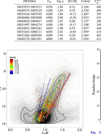
Figure 2 shows the 2MASS colour–magnitude diagram (H vs. J − K) for Baade’s window. The APOGEE and DR1-GES samples are colour-coded as a function of metallicity. We also show the PARSEC isochrones (Bressan et al. 2012), assum-ing an age of 10 Gyr, with varyassum-ing metallicities assumassum-ing that the stars in BW have a mean distance of 8.4 kpc (Chatzopoulos et al. 2015). We assume an average extinction of AV = 1.5 (Stanek 1996), and the reddening law ofNishiyama et al.(2009), which we used to redden the isochrones. Stars with log g > 3.5 have been excluded. We see clearly that the APOGEE stars have redder (J − K)0 colours than predicted by the most metal-rich isochrones (Z= 0.07). While the metal-poor stars generally have bluer (J − K) colours, stars with similar spectroscopically deter-mined metallicities show a wide range in the (J − K) colour.

2.2. Comparison samples

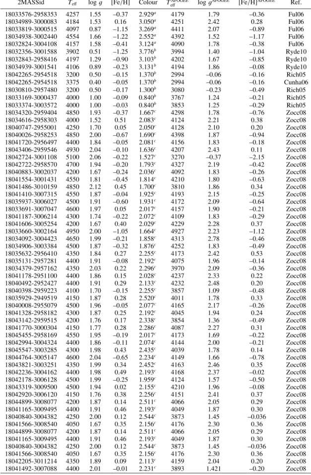
As mentioned in Sect. 2.1, BW was targeted by APOGEE for calibration with respect to studies having well-established stellar parameters and chemical abundances. For the cross-identification of coordinates and 2MASS IDs of our stars, we used Table 1 ofChurch et al.(2011), who provided coordinates and 2MASS names for all stars in Arp’s finding chart (Arp 1965). Fulbright et al. (2006) obtained effective temperatures based on V − K data, together with the photometric transforma-tion to TefffromAlonso et al.(1999). In total we have five stars in common with Fulbright et al. (2006, hereafter Ful06), four stars withRich & Origlia(2005, hereafter Rich05), three with Ryde et al.(2010, hereafter Ryde10), one withCunha & Smith (2006, hereafter Cunha06), and 55 with Zoccali et al. (2008, hereafter Zocc08). The right panel of Fig. 1displays the posi-tion of the individual stars in all these studies. The region dis-played corresponds to that highlighted by a white square in the left panel of the same figure. Table1lists the stellar parameters of the different literature values, as well as those from APOGEE (DR13,SDSS Collaboration et al. 2016).

Table 1. Comparison of stellar parameters.

2MASSid Teff log g [Fe/H] Colour TAPOGEE

eff log gAPOGEE [Fe/H]APOGEE Ref.

18033576-2958353 4257 1.55 –0.37 2.929a _{4179 1.79 –0.36 Ful06} 18034989-3000083 4184 1.53 0.16 3.050a _{4251 2.42 0.28 Ful06} 18033819-3000515 4097 0.87 –1.15 3.269a _{4411 2.07 –0.89 Ful06} 18034938-3002440 4554 1.66 –1.22 2.552a _{4392 1.52 –1.17 Ful06} 18032824-3004108 4157 1.58 –0.41 3.124a _{4090 1.78 –0.38 Ful06} 18032356-3001588 3902 0.51 –1.25 3.776b _{3994 1.40 –1.04 Ryde10} 18032843-2958416 4197 1.29 –0.90 3.103b _{4202 1.67 –0.85 Ryde10} 18034939-3001541 4106 0.89 –0.23 3.131b _{4194 1.86 –0.08 Ryde10} 18042265-2954518 3200 0.50 –0.15 1.370b _{2994 –0.06 –0.16 Rich05} 18042265-2954518 3375 0.40 –0.05 1.370b _{2994 –0.06 –0.16 Cunha06} 18030810-2957480 3200 0.50 –0.17 1.300b _{3080 –0.23 –0.49 Rich05} 18033169-3000437 4000 1.00 –0.09 0.840b _{3767 1.24 –0.21 Rich05} 18033374-3003572 4000 1.00 –0.03 0.840b _{3853 1.25 –0.29 Rich05} 18034320-2959404 4850 1.93 –0.37 1.667c _{4298 1.78 –0.76 Zocc08} 18034616-2958303 4000 1.52 0.51 2.083c _{4124 2.21 0.38 Zocc08} 18040747-2955001 4250 1.70 0.05 2.050c _{4128 2.10 0.20 Zocc08} 18040026-2958253 4850 2.00 –0.67 1.690c _{4398 1.87 –0.94 Zocc08} 18041720-2956497 4400 1.84 –0.05 2.081c _{4156 1.83 –0.18 Zocc08} 18043406-2959546 4930 2.04 –0.10 1.636c _{4207 2.43 0.11 Zocc08} 18042724-3001108 5100 2.06 –0.22 1.527c _{3270 –0.37 –2.15 Zocc08} 18042722-2958570 4700 1.94 –0.20 1.793c _{4327 2.19 –0.42 Zocc08} 18040883-3002037 4200 1.67 –0.24 2.036c _{4092 1.83 –0.26 Zocc08} 18041554-3001431 4550 1.81 –0.45 1.814c _{4210 1.80 –0.63 Zocc08} 18041486-3010159 4850 2.12 0.45 1.700c _{3810 1.86 0.34 Zocc08} 18041410-3007315 4550 1.87 –0.04 1.925c _{4193 2.15 –0.25 Zocc08} 18035937-3006027 4500 1.91 –0.60 1.931c _{4172 2.09 –0.64 Zocc08} 18033691-3007047 4600 1.97 0.05 2.017c _{4157 1.90 –0.21 Zocc08} 18041187-3006214 4300 1.74 –0.22 2.072c _{4109 1.83 –0.29 Zocc08} 18041606-3005254 4200 1.67 0.40 2.029c _{4229 2.28 0.37 Zocc08} 18033660-3002164 4950 2.00 –1.05 1.664c _{4927 2.23 –1.12 Zocc08} 18034092-3004423 4650 1.99 –0.21 1.858c _{4313 2.78 –0.46 Zocc08} 18034906-3003384 4500 1.87 –0.32 1.876c _{4252 1.83 –0.49 Zocc08} 18035632-2956410 4350 1.84 0.27 2.255c _{4173 2.42 0.53 Zocc08} 18035131-2957281 4400 1.91 –0.08 2.192c _{4075 1.96 –0.14 Zocc08} 18034379-2957162 4350 2.03 0.22 2.296c _{3970 2.09 –0.36 Zocc08} 18041178-2951100 4400 1.86 0.15 2.028c _{4237 2.33 0.22 Zocc08} 18040492-2952427 4400 1.91 0.29 2.133c _{4232 2.48 0.20 Zocc08} 18040398-2959223 4100 1.70 –0.15 2.255c _{3857 1.09 –0.48 Zocc08} 18035929-2949519 4150 1.87 0.28 2.520c _{4011 1.78 0.33 Zocc08} 18040008-2955079 4500 1.96 –0.05 2.077c _{4165 2.17 –0.26 Zocc08} 18041328-2958182 4300 1.87 0.25 2.192c _{4045 1.94 0.24 Zocc08} 18043142-2959515 4200 1.76 0.17 2.338c _{3854 1.36 –0.49 Zocc08} 18041770-3000304 4150 1.77 0.28 2.286c _{4087 2.27 0.31 Zocc08} 18045455-2958169 4550 1.95 –0.19 2.017c _{4173 1.69 –0.22 Zocc08} 18042994-3004324 4400 1.86 –0.11 2.074c _{4144 2.00 –0.21 Zocc08} 18045547-3003285 4300 1.98 0.43 2.435c _{4039 1.78 0.14 Zocc08} 18044764-3005147 4600 2.04 –0.65 2.234c _{4149 1.66 –0.78 Zocc08} 18043821-3003251 4350 1.99 0.34 2.452c _{4163 2.46 0.35 Zocc08} 18042236-3004162 4400 1.98 0.49 2.193c _{4168 2.37 –0.02 Zocc08} 18042178-3006128 4500 1.99 –0.25 1.959c _{4124 1.57 –0.50 Zocc08} 18043319-3009500 4500 1.94 0.02 2.155c _{4210 1.96 –0.08 Zocc08} 18042920-3006120 4150 1.76 0.38 2.256c _{4151 2.41 0.37 Zocc08} 18044899-3008077 4200 1.87 0.14 2.511c _{4066 2.05 0.29 Zocc08} 18041165-3009495 4400 1.91 0.46 2.193c _{4049 1.87 0.30 Zocc08} 18040840-3004382 4250 2.00 0.12 2.544c _{3873 1.45 –0.036 Zocc08} 18041566-3008540 4050 1.67 0.35 2.156c _{4176 2.30 0.36 Zocc08} 18044899-3008077 4200 1.87 0.14 2.511c _{4066 2.05 0.29 Zocc08} 18041165-3009495 4400 1.91 0.46 2.193c _{4049 1.87 0.30 Zocc08} 18040840-3004382 4250 2.00 0.12 2.544c _{3873 1.45 –0.036 Zocc08} 18041566-3008540 4050 1.67 0.35 2.156c _{4176 2.30 0.36 Zocc08} 18042205-3011214 4350 1.89 0.09 2.113c _{4159 2.04 0.20 Zocc08} 18041492-3007088 4400 2.01 –0.01 2.231c _{3893 1.421 –0.20 Zocc08}

Notes. Columns 2–4 list the stellar parameters as derived in the reference quoted in the last column. The APOGEE stellar parameters are listed in Cols. 5–7.(a)_{(V − K)}

Table 1. continued.

2MASSid Teff log g [Fe/H] Colour TAPOGEE

eff log gAPOGEE [Fe/H]APOGEE Ref.

18035975-3007473 4350 1.88 0.31 2.256c _{4046 1.84 0.24 Zocc08} 18040535-3005529 4100 1.84 0.35 2.530c _{4049 2.27 0.50 Zocc08} 18034164-3007549 4200 1.80 –0.12 2.407c _{3959 1.805 0.19 Zocc08} 18040486-3003009 4500 2.00 –0.20 2.032c _{4105 1.87 –0.61 Zocc08} 18040030-3004017 4300 1.85 0.08 2.157c _{3964 1.89 -0.73 Zocc08} 18031997-3004274 4300 1.98 –0.17 2.398c _{3849 1.26 –0.30 Zocc08} 18034052-3003281 4450 1.90 0.55 1.857c _{4486 2.24 –0.90 Zocc08} 18031683-3006111 4650 2.02 –0.05 1.959c _{4181 1.95 –0.34 Zocc08} 18033286-3005450 4200 1.94 0.28 2.384c _{4037 2.11 0.34 Zocc08} 18040170-3001491 4600 1.99 –0.01 1.954c _{4118 2.65 –0.03 Zocc08}

Fig. 2.2MASS H vs. J − K diagram for stars in BW. Superimposed over the individual star measurements are the density contours. The APOGEE targets are shown as filled circles; the GES targets are shown as open circles. The colour scale indicates the metallicity of the stars. Superimposed are the 10 Gyr PARSEC isochrones for different metal-licities, colour-coded as in the legend.

3. Distances

The spectrophotometric distances and reddenings for the full sample were calculated using the stellar parameters Teff, log g, and [Fe/H], together with 2MASS J, H, and KS photometry and associated errors, to simultaneously compute the most likely line-of-sight distance and reddening by isochrone fitting with a set of PARSEC isochrones. We used the same method as pre-sented in Rojas-Arriagada et al. (2017), considering a set of isochrones in the age range from 1 to 13 Gyr in 1 Gyr steps and metallicities from −2.2 to+0.5 in steps of 0.1 dex. We chose this method to calculate the distances consistently with respect to the bulge sample of the GES. A comparison was made with the distance code of the “BPG group” (Santiago et al. 2016), which uses a Bayesian approach. We did not find any systematic offset in the distance distribution.

Figure3displays the histogram of our BW sample as grey bars. The peak of the histogram is located close to the distance of the Galactic Centre (RGC= 0 kpc), and then decreases towards

0 2 4 6 8 10 12 14 RGC(kpc) 0 10 20 30 40 50 Number -bulge Bulge Thick disk Thin disk 0 200 400 600 800 1000 1200 1400 1600 Number -disk

Fig. 3. Distribution of the Galactocentric distances of our

APOGEE sample. Grey bars indicate bulge stars (according to the left vertical scale), while the blue and red open histograms show the thick and the thin disc (according to the right vertical scale), respectively. The vertical dashed line defines our cut at RGC = 3.5 kpc to select likely bulge stars, while the vertical dotted line represents our cut at RGC = 7.7 kpc used to select the comparison disc sample (see Sect. 6).

larger distances. For the discussion of the MDF (Sect. 5) we restrict our sample to RGC < 3.5 kpc to ensure a sample of stars likely located in the Galactic bulge. This selection criterion leaves us with 269 stars. The two open histograms in Fig.3show the distribution of APOGEE disc stars, from which we selected a comparison subsample. The definition of this disc sample is discussed in Sect.6.

4. Comparison of stellar parameters

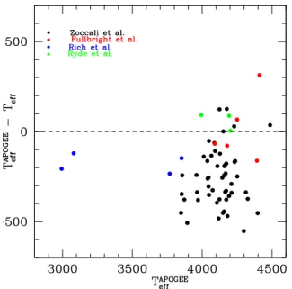
Figure4 presents the comparison of the effective temperatures between Rich05, Ful06, Zocc08, and Ryde10. Table2gives the corresponding mean differences and the standard deviation of the stellar parameters with respect to APOGEE. The Rich05 and the Zocc08 stars exhibit systematically higher tempera-tures (177 K and 255 K, respectively) compared to APOGEE, while Ful06 and Ryde10 obtain similar temperatures (15 K and 61 K). The largest dispersion appears for the Ful06 stars and for the Zocc08 stars (186 K and 161 K, see Table 2), while

Fig. 4.Difference in Teff between APOGEE and literature values vs. Teff. Black circles are giants from Zoccali et al. (2008), red circles are fromFulbright et al.(2006), blue circles are fromRich & Origlia

(2005), and green circles are fromRyde et al.(2010).

the dispersion in Ryde10 and Rich05 is rather small (49 K and 52 K). In our comparison sample (see Fig. 4), the e ffec-tive temperatures of Ful06 were determined based on photomet-ric V − K colours, and on differential excitation temperatures and ionization temperatures. They found in general a very good agreement between these three temperature estimates with a small scatter. Zocc08 uses V − I colours as a first estimate, while the final Zocc08 values, which we adopted here for comparison, were estimated spectroscopically by imposing excitation equi-librium on a set of ∼60 FeI lines. Rich05 estimated temperatures based on J − K colours, while Ryde10 uses the effective temper-atures of Ful06.

One part of the wide range of photometric temperatures com-pared to the spectroscopic values of APOGEE can be explained by the inhomogeneous use of photometric colours in the compar-ison work, while the spectroscopic temperatures from APOGEE were determined in a homogeneous way. We indicate in Table1 the corresponding photometric colours as well as the photomet-ric system used.González Hernández & Bonifacio(2009) stud-ied in detail the effective temperature scale using the infrared flux method. They show in their Table 5 that the V − K colours show the smallest dispersion in the determination of the e ffec-tive temperature (∼30 K) and should therefore be used for pho-tometric temperatures. The V − I colours and especially the J − K colours show, on the other hand, a much larger disper-sion in the effective temperature. Clearly, much more effort is needed to understand the difference between spectroscopic and photometric temperature determinations.

Figure5shows the APOGEE-literature comparison of sur-face gravity. The sursur-face gravities of APOGEE are calibrated with respect to the asteroseismic log g estimates from NASA’s Keplermission (Borucki et al. 2010). The applied offset is about 0.2 dex for stars with solar metallicities. The typical dispersion between photometric log g and spectroscopic estimates are of the order of ±0.5 dex, while the dispersion in Ryde10 is slightly lower (0.3 dex) although they exhibit a large offset (0.62 dex). In general, there is a large systematic discrepancy between photo-metrically derived log g and spectroscopic estimates.

Table 2. Difference between stellar parameters from APOGEE com-pared to the literature (∆) and its rms dispersions of the differences (σ) for stellar parameters Teff, log g, [Fe/H], and α.

Rich05 Ful06 Zocc08 Ryde10

h∆Teffi –177 15 –255 61 [K] σ(Teff) 52 186 161 49 [K] h∆ log gi –0.19 0.48 –0.12 0.62 [dex] σ(log g) 0.52 0.54 0.48 0.29 [dex] h∆[Fe/H]i –0.18 0.13 0.10 0.18 [dex] σ([Fe/H]) 0.14 0.09 0.28 0.09 [dex] h∆[α/Fe]i –0.19 –0.19 –0.07 –0.13 [dex] σ([α/Fe]) 0.11 0.10 0.15 0.06 [dex]

Fig. 5.Difference in log g between APOGEE and literature values vs.

log g using the same symbols as in Fig.4. A clear linear relation is seen for the Zocc08 sample between the difference of the spectroscopic and photometric gravities with respect to the spectroscopic log g values (see text).

The Zocc08 photometric log g estimates display a clear lin-ear behaviour with respect to APOGEE. In Zocc08, the photo-metric gravities were estimated by assuming a mean stellar mass of M = 0.8 M and a sample distance of 8 kpc. The disper-sion of their log g is about 0.25 dex and is due to the intrinsic depth of the Galactic bulge (Lecureur et al. 2007). We investi-gate the effects of these assumptions by selecting stars from a TRILEGAL (Girardi et al. 2012) simulation using the Zocc08 photometric selection function (see their Fig. 1), and calculating photometric log g values. Figure 6 displays the selected simu-lated stars in the same plane as in Fig.5, colour-coded by the difference of their true distances with respect to an assumed mean field distance (dBW). Given the relatively narrow magni-tude selection of Zocc08, stars at greater distances than dBW are intrinsically luminous (low log g values), but appear fainter. By assuming these stars are at dBW, the resulting photometric log g values are higher, to account for their apparent low lumi-nosity, determining a∆log g(true − phot) < 0. Conversely, fore-ground stars at distances shorter than dBW, are on average intrin-sically less luminous (high log g values). By assuming these stars are at dBW, the resulting photometric log g values are smaller,

0.0 0.5 1.0 1.5 2.0 2.5 3.0 3.5

log(g)

log

(g)

−

log

(g)

d

−

d

Fig. 6.Difference in log g for stars selected from a TRILEGAL

simu-lation of BW as a function of log g (true). The photometric values were computed by assuming the whole sample is at a distance of 8 kpc. Sym-bols are colour-coded according to the difference of the true distance with respect to that assumption. Photometric gravities become smaller with respect to the true spectroscopic surface gravities if the assumed distance is shorter than 8 kpc.

to account for their apparent high luminosity, determining a ∆log g(phot − spec) > 0. The interplay between these comple-mentary effects determines the linear trend observed in Fig.5 and reproduced in Fig.6. The dispersion around the mean oc-curs because for a given distance interval there are stars spanning a range of true log g values. If we consider that the reddening in BW is small and homogeneous, photometric log g estimates in other windows of the Galactic bulge, where interstellar ex-tinction is higher and spatially patchy, could lead to even larger uncertainties.

Figure7 shows the comparison of the global metallicities. Except for Rich05, the comparison samples predict metallicities that are generally too low with respect to APOGEE. The o ff-set can go up to 0.18 dex (Ryde10). The typical dispersion is about 0.15 dex, but is significantly larger for the Zocc08 sam-ple (0.28 dex), where stars with [M/H] < 0 are systematically more metal-poor with respect to the APOGEE measurements. This larger scatter is partially due to the larger dispersion in Teff and log g (see Figs.4and5) of the Zocc08 determinations.

For the comparison of the α-elements, we used the combi-nation of Mg and Si for Rich05 and Ful06, the Gonzalez et al. (2011a) values for the Zocc08 sample, and the global α-element estimate for Ryde10. In general, the α-element abundances in APOGEE are lower than the literature values with differences ranging from 0.07 dex (Zocc08) up to 0.19 dex (Rich05, Ful06). The dispersion is about 0.1 dex, where again Zocc08 has a larger dispersion (0.15 dex).

5. Metallicity distribution function

The MDF of BW stars is an important tool that can be used to unravel the mix of stellar populations that comprise the Galac-tic bulge. With larger sample sizes, it becomes clear that the MDF does not reflect a single stellar population, but reveals at least a bimodal nature. This behaviour was previously no-ticed by Hill et al. (2011), and was further characterized by Babusiaux et al. (2010), who found metal-rich stars display-ing bar-like kinematics in contrast with the isotropically hotter metal-poor bulge.

Fig. 7.Difference in [Fe/H] between APOGEE and literature values vs. [Fe/H] using the same symbols as in Fig.4. The typical dispersion is about 0.1 dex, while the dispersion increases significantly for the Zocc08 sample (∼0.28 dex).

Fig. 8.Difference in [α/Fe] between APOGEE and literature values vs.

[α/Fe]. The symbols are the same as in Fig.4. The typical dispersion is 0.1 dex, with a slightly higher value for the Zocc08 sample (∼0.15 dex).

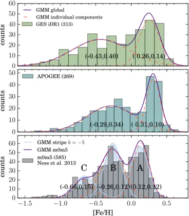
Figure9 compares the BW MDF as sampled by APOGEE with two other recent large-scale spectroscopic surveys, the ARGOS (in m0m5, a field close to BW; Freeman et al. 2013; Ness et al. 2013) and the GES (iDR1 Gilmore et al. 2012; Rojas-Arriagada et al. 2014; Mikolaitis et al. 2014). In each case, we used spectrophotometric distances to select samples of likely bulge stars as those with Galactocentric distance sat-isfying RGC < 3.5 kpc, as was done for the APOGEE sample (Sect. 3). The visual inspection of the metallicity distributions of these likely bulge stars, as depicted by the histograms in each panel, reveals some qualitative differences. While the GES and

0 10 20 30 40 50 60 counts (-0.43,0.40) ( 0.26,0.14) GMM global GMM individual components GES iDR1 (313) 0 10 20 30 40 50 counts (-0.29,0.34) ( 0.31,0.10) APOGEE (269) −1.5 −1.0 −0.5 0.0 0.5 [Fe/H] 0 10 20 30 40 50 60 counts

A

B

C

Fig. 9.Metallicity distribution function for stars in BW. Only sources with RGC < 3.5 kpc are included. Top panel: MDF of the GES BW data (iDR1). Middle panel: MDF of the APOGEE data. In each case, the GMM decomposition is depicted by dashed (individual compo-nents) and solid (global profile) lines, with mean and width values in parentheses. Lower panel: MDF of the closest field to BW from AR-GOS data (Ness et al. 2013). The GMM decomposition is depicted as in the other panels. For comparison, the GMM decomposition of the b = −5◦

strip, as taken from Ness et al.(2013), is depicted by the three Gaussian profiles, with the corresponding mean and width values quoted in parentheses.

APOGEE samples can be described with bimodal distributions, the ARGOS sample apparently requires a third component.

To quantify the substructure of the different MDFs, we per-form a Gaussian mixture model (GMM) decomposition indepen-dently for each case. A GMM is a parametric probability density function given by a weighted sum of a number of Gaussian com-ponents. The GMM parameters are estimated as those that pro-vide the best representation of the data set density distribution structure. The expectation-maximization algorithm determines the best parameters of a mixture model for a given number of components. Since, in the general case, the number of compo-nents is not known beforehand, an extra loop of optimization is required to compare several optimal models with different num-bers of components. To perform this task, we adopted the Akaike information criterion (AIC) as a cost function to asses the rel-ative fitting quality between different proposed mixtures. In the case of the GES and APOGEE samples, the AIC gave preference for a two-component solution with centroid and width values as quoted in each panel. The narrow metal-rich component is quite similar in both data sets, while the metal-poor one is broader and relatively more metal-poor in the GES data.

The ARGOS MDF was found in Ness et al. (2013) to be composed of up to five metallicity components, with the three most metal-rich (designated as A, B, and C: [Fe/H] > −1.0 dex) accounting for the majority of stars. In that work, three gen-eral MDFs were assembled from samples in fields located in

three latitude stripes (±15◦ in longitude) at b = −5o, −7.5o, and −10o_{. Their GMM analysis yielded a three-component} so-lution in each case. In particular, in the lower panel of Fig.9, we display in light blue the three Gaussian components resulting from their analysis of the b = −5o _{stripe. For verification, we} performed a GMM analysis on the m0m5 field sample, which is depicted by the histogram. The best model is a mixture of three Gaussians with means of µ= −0.69, −0.27, 0.14 and dispersions of σ= 0.14 dex, 0.16 dex, 0.11 dex, in good agreement with the Ness et al.(2013) results for the entire b= −5o strip, as quoted in the lower panel of Fig.9.

The trimodal metallicity distribution of the ARGOS data is visible in the individual field distributions and in the merged strip samples. This feature might be an imprint of the parametriza-tion performed on the ARGOS data, but it could also arise as an effect of assembling samples over a large longitudinal area where small systematic variations in the intrinsic shape of the bulge MDF are possible. In particular, the trimodal nature of the ARGOS parametrization could come from the fact that ARGOS uses effective temperature estimates from (J − K)0colours (Freeman et al. 2013), which can result in sys-tematic differences (see Fig.4) compared to spectroscopically derived temperatures.Recio-Blanco et al.(2016) estimated the end-of-mission expected parametrization performances of the Gaia DPAC pipeline (GSP-Spec) used for the derivation of the atmospheric parameters and chemical abundances from the RVS stellar spectra (R = 11 200). The spectral resolution, as well as the spectral region, of the Gaia-RVS is very similar to that of ARGOS. Recio-Blanco et al.(2016) showed, based on model spectra (see their Fig. 21), that an error of 100 K can easily result in at least 0.1 dex errors in [Fe/H] with a signifi-cantly large dispersion that gets larger for cooler stars. An effect such as this could be the reason for the additional third compo-nent in the observed MDF of ARGOS. On the other hand, the bimodality of the bulge MDF has been characterized by a num-ber of studies examining specific locations in the bulge region (Uttenthaler et al. 2012;Gonzalez et al. 2015), and by the results of the fourth internal data release of the GES (Rojas-Arriagada et al.2017), which covers a larger area. To understand the di ffer-ence between the ARGOS data set and those of APOGEE and GES, a common set of observed stars covering the full metal-licity range – which is currently not available – is necessary. In the end, this discrepancy highlights that understanding the number of metallicity-distinguished components constituting the bulge is an important and unresolved issue warranting further investigation.

6. Trends in the abundance-metallicity plane

The distribution of stars from a given population in the abundance-metallicity plane encodes important information about its star-formation history and chemical evolution. In par-ticular, detailed comparisons between the bulge and other Galac-tic components in the [α/Fe] vs. [Fe/H] plane can provide a di-rect means of unraveling the origin of the bulge in the context of other Galactic stellar populations.

Figure 10 displays our BW APOGEE sample in the

[Mg/Fe] vs. [Fe/H] plane. To compare this data with the GES, we overplot the median trend of its BW stars, as determined by di-viding the sample into narrow metallicity bins (Rojas-Arriagada et al.2017). To assess the statistical significance of the result-ing profile, a shaded area depicts the standard error of the mean. To enhance the comparison, we computed in the same man-ner the median trend of the bulge APOGEE sample studied

−1.5 −1.0 −0.5 0.0 0.5 [Fe/H] −0.3 −0.2 −0.1 0.0 0.1 0.2 0.3 0.4 0.5 [Mg/F e]

APOGEE-BW mean curve GES p1m4 mean curve APOGEE-BW

Fig. 10.Baade’s window stars in the [Mg/Fe] vs. [Fe/H] plane. The

APOGEE sample and its median trend (blue open circles and blue line, respectively) are compared with the mean trend of BW stars from the fourth internal data release of the GES (red line). A shaded red area around the mean trend depicts the standard error of the mean.

here. The abundance scale of APOGEE agrees remarkably well with that of the GES. The GES stars are on average slightly less α-enhanced than APOGEE stars, by about 0.02 dex over the common metallicity range. There is a clear discrepancy be-tween the α-element abundances bebe-tween APOGEE and GES for the more metal-rich stars ([Fe/H] > −0.1), in the sense that the GES obtains lower α-element abundances. The difference is ∼0.1 dex at [Fe/H] = +0.2 and increases to ∼0.15 dex at [Fe/H] = +0.4 dex. APOGEE derives Mg abundances from four different spectral windows (centred at 1.533, 1.595, 1.672, 1.676 µm), all of them in the infrared H band (see García Pérez et al. 2016), while GES uses the lines at 8717.8 Å, 8736.0 Å, and 8806.7 Å in the optical spectral range. A part of the differences between APOGEE and GES could arise from differences in atomic data, although one has to be aware that abundance determination for metal-rich giants, like those used in these two studies, is chal-lenging and systematic effects from other sources would not be surprising.

This comparison emphasizes the necessity of a common sample of stars well-distributed in the Teff-log(g)-[Fe/H] space to cross-calibrate abundance measures coming from different surveys.

In Fig.11we attempt a direct homogeneous comparison be-tween the distributions of disc and bulge stars in the abundance-metallicity plane, using results exclusively from APOGEE. To this end, we selected a sample of disc stars (namely, stars in pointings with |l| ≥ 15o and |b| ≥ 15o), cleaning it based on several flags provided by the ASPCAP pipeline. In addition, we selected stars with RGC < 7.7 kpc (dotted line in Fig. 3) to have a sample representing the chemical distributions inside the solar circle, without decreasing the sample size significantly. To minimize the systematics arising from the comparison of stars with different fundamental parameters, we selected disc stars in the same range of Teff and log g spanned by our BW sample. Application of all of the previous cuts yield a final sample of 2904 stars.

The selected disc stars present a distribution in the abundance-metallicity plane with a clear gap separating a high-α and low-α sequences (see also Hayden et al. 2015). We divide the sample by performing a clustering analysis in narrow metal-licity bins. The resulting thin- and thick-disc samples (brown and blue points, respectively), together with the BW bulge sample (red crosses), are depicted in Fig.11. To aid visualization of their

−1.5 −1.0 −0.5 0.0 0.5 [Fe/H] −0.1 0.0 0.1 0.2 0.3 0.4 [Mg/F e] Bulge-BW (269) Thick disk (1628) Thin disk (1276)

Fig. 11.[Mg/Fe] vs. [Fe/H] for thin disc (brown points), thick disc (blue points), and BW (red crosses) stars. Median trends are computed for the discs (dashed lines) and the bulge (solid line) in small metallicity bins as a visual aid. Bulge stars appear to be on average more α-enhanced than the thick disc.

distributions, we compute a median trend for the discs (dashed lines) and the bulge (solid line). Interestingly, bulge stars appear to be on average more α-enhanced than the thick disc, reaching higher metallicity values. This may be the result of a difference in the relative formation timescales, where that of the bulge is faster and dominated by massive stars. The confirmation of this feature is of clear importance in our quest for disentangling the different natures and origins of the stellar populations that co-exist in the central kiloparsecs of the Galaxy.

There are a small number of stars with low magnesium abun-dances. Their relative proportion does not decrease significantly if we apply a more stringent cut in Galactocentric distances, which means that if we account for the large errors in spec-trophotometric distances these stars appear to be located inside the bulge region. Recio-Blanco et al. (2017) found from GES Bulge data a small fraction of low-α stars that have chemical pat-terns compatible with those of the thin disc, indicating a complex formation process of the Galactic bulge.

7. Age distribution

Obtaining accurate ages for stars in the Galactic bulge is a cru-cial ingredient in the comparison of observed data to chemo-dynamical evolutionary models. Recently,Martig et al. (2016) developed a new method for estimating masses and implied ages for giant stars based on C and N abundances calibrated on astero-seismic data. They demonstrate that the [C/N] ratio of giants decreases with increasing stellar mass, as expected from stellar-evolution models. We use the relation of Martig et al. (2016) from Appendix A.3, and adopt the same cuts as those authors to ensure the reliability of the relation: 4000 < Teff < 5000 K, 1.8 < log g < 3.3, [M/H] > −0.8, −0.25 < [C/M] < 0.15, −0.1 < [N/M] < 0.45, −0.1 < [(C + N)/M] < 0.15, and −0.6 < [C/N] < 0.2. This leaves only 74 stars; Fig.12shows the age distribution of stars with metallicity lower and higher than [Fe/H]= −0.1 dex3(to roughly separate stars into the two modes of the MDF; see Fig.9). Given the small size of the sam-ple, we use generalized histograms (kernel of 1.5 Gyr) to avoid the effect of binning of conventional histograms, and a boot-strap analysis to asses for the significance of the resulting dis-tributions. To this end, we performed 600 bootstrap resamplings 3 _{The results below do not qualitatively change if the cut is done at} ±0.1 dex from this limit.

2 4 6 8 10 12 Age (Gyr) 0.00 0.02 0.04 0.06 0.08 0.10 0.12 Density metal-rich [Fe/H]>-0.1 metal-poor [Fe/H]<-0.1 Kernel = 1.5 Gyr

Fig. 12. Age distribution of stars in BW using the formula of

Martig et al.(2016). Only sources with 4000 < Teff < 5000 K, 1.8 < log g < 3.3, [M/H] > −0.8, −0.25 < [C/M] < 0.15, −0.1 < [N/M] < 0.45, −0.1 < [(C+ N)/M] < 0.15, and −0.6 < [C/N] < 0.2 were taken into account. From a bootstrap analysis on generalized histograms (kernel 1.5 Gyr), mean trends (solid and dashed grey lines), and error bands to the ±2σ level (shaded coloured areas) are derived for metal-rich and metal-poor stars (cut at [Fe/H] = −0.1 dex) as percentiles of the 600 bootstrap resamplings.

of the metal-rich and metal-poor samples, computing median trends (solid and dashed grey lines) and error bands (shaded ar-eas) at the ±2σ level from percentiles.

The peak of the distribution of metal-poor stars is about ∼10 Gyr, with a decreasing tail toward younger ages. This compares well with the mean bulge age as estimated from photometric data (Zoccali et al. 2003; Clarkson et al. 2008, Valenti et al. 2013). On the other hand, the generalized dis-tribution of metal-rich stars shows a flatter disdis-tribution, with two overdensities of young and old stars. This seemingly bi-modal age distribution for metal-rich stars is comparable with the results ofBensby et al.(2013), who found from their sam-ple of dwarf and subgiant microlensed stars that while metal-poor bulge stars are uniformly old, metal-rich bulge stars span a broad range of ages (2−12 Gyr), with a peak at 4−5 Gyr. Re-cently, Haywood et al.(2016) concluded, from deep HST data in the SWEEPS field, that a certain fraction of young stars is necessary to reproduce the observed colour-magnitude diagram (CMD). In their model, about 50% of the stars have ages greater than 8 Gyr, suggesting that there might be a fraction of young stars in their CMD. If we extrapolate their results to BWs, ac-cording to their model we would expect 35% of the stars to be younger than 8 Gyr. We find a very similar fraction to that seen in Fig. 12. However, their model reports that metal-rich stars with [Fe/H] > 0.0 are all younger than 8 Gyr, while our small sample suggests that metal-rich stars can be either young or old. We also note that the younger population exhibit, on average, less α-element enhancement than the old population (alphamean = 0.126 for ages < 6 Gyr and alpha = 0.215 for ages > 6 Gyr). Overall, our age distributions derived from chem-istry seem robust, despite the sample size, and constitute an inde-pendent verification of results suggested from isochrone fitting to fundamental parameters (Bensby et al. 2013) and photomet-ric data (Haywood et al. 2016). However, we want to stress that the ages derived from [C/N] abundances have to be considered

with caution. As discussed byMartig et al.(2016), the absolute scaling of the derived ages might be slightly off. This leads, for example, to underestimated ages of old stars, as shown in their Fig.11. In addition, owing to our small sample of stars, more data are clearly necessary to better constrain the bulge age dis-tribution and its metallicity dependence.

8. Individual chemical abundances

Compared to the 15 individual elemental abundances determined in DR12 (Holtzman et al. 2015), the DR13 results include seven new elements: P, Cr, Co, Cu, Ge, Rb, and Nd; in total, DR13 includes elemental abundances for the 22 elements C, N, O, Na, Mg, Al, Si, P, S, K, Ca, Ti, V, Cr, Mn, Co, Ni, Cu, Ge, Rb, Y, and Nd. However, we only discuss the abundances for 11 of these elements in this section. The reasons for the exclusion of the other 11 elements are as follows:

– We do not include C and N abundances because a giant star which ascends the giant branch deepens the convective enve-lope and the star experiences the first dredge-up. This means that CNO-processed material containing a lot of N but de-pleted in C is brought to the surface. This is nicely shown in Fig. 1 ofMartig et al.(2016). It also turns out that the depth of the convective envelope and the amount of CNO-cycling in the core depends on the mass of the star, a fact that we use to get ages for the stars in our Sect. 7. This means that giants cannot be used to trace the galactic chemical evolution of C and N: the abundances simply do not reflect the abundances of their birth. This is shown in the lower panel of Fig. 2 in Martig et al.(2016).

– The spectral lines used to determine the P abundances are generally very weak in the type of giants observed in BW. Holtzman et al. (in prep.) caution that these lines are weak and uncertain, whileHawkins et al.(2016) derive only upper limits in their independent analysis of APOGEE spectra. We therefore exclude this element in the discussion below. – The abundance-trend of S for the BW stars is very scattered

as compared to our sample of local disc stars, possibly be-cause the S abundance is in principle derived from a single, blended line, and higher S/N than the already high S/N of the BW spectra are needed to trace this element with certainty. We therefore exclude this element in the discussion below. – The DR13 abundance trends of Ti in the local discs do

not resemble the expected α-element trends found in many other works. The reason for this behaviour is described in Hawkins et al. (2016), as possible 3D/NLTE-effects in the Ti I lines used in DR13. We therefore exclude this element in the discussion below.

– The abundance trend of V in the BW stars is very scattered. The V abundances are mainly determined from two lines, of which one is quite weak but the other is of suitable strength. It is possible that the V abundance trend in the bulge would be less scattered if the weak line were to be excluded in the analysis. We also note that Hawkins et al.(2016) derive a different V trend for their independent analysis of a subsam-ple of APOGEE-spectra. For these reasons, we exclude this element in the discussion below.

– The Cu, Ge, Rb, Y, and Nd abundances are all determined from few, often single, weak and blended lines. We therefore exclude these elements in the discussion below.

To conclude, we discuss the abundances of the following 11 el-ements in this section: O, Na, Mg, Al, Si, K, Ca, Cr, Mn, Co, and Ni.

Fig. 13.[Fe/H] vs. [X/Fe] of APOGEE stars in BW for α-elements compared with literature values.

8.1. Theα-elements: O, Mg, Si, and Ca

Figure 13shows the trends of the α-elements (O, Mg, Si, Ca) compared to available literature values for M giants. These abun-dances are of particular interest because accurate [α/Fe] ra-tios place strong constraints on the star-formation history (e.g. Matteucci & Brocato 1990) in a stellar population. In addi-tion to the previously menaddi-tioned references, we add that of Jönsson et al.(2017), who determined elemental abundances of O, Mg, and Ca of bulge K giants using the high-resolution (R ∼ 47 000) UVES/FLAMES spectrograph at the VLT.

Oxygen abundances determined in Rich05, Cunha06, Fulbright et al. (2007b), Ryde10, andJönsson et al.(2017) are presented in the top left panel of Fig.13. The APOGEE O abun-dances are lower than those of Rich05 and Fulbright et al. (2007b), while they are comparable to those of Cunha06, Ryde10, andJönsson et al.(2017).

Magnesium abundances are determined in Rich05, Fulbright et al. (2007b), Gonzalez et al. (2011a), Hill et al. (2011), and Jönsson et al. (2017); these abundances are displayed in the top right panel of Fig. 13. The APOGEE Mg abundances exhibit generally good agreement with the trends found by Gonzalez et al. (2011a) and Hill et al. (2011). The Rich05, Fulbright et al.(2007b), and possiblyJönsson et al.(2017) stars are slightly enhanced in Mg compared to APOGEE, in particular in the metal-rich regime ([Fe/H] > 0.2).

Silicon abundances are determined in Rich05, Fulbright et al. (2007b), Ryde10, and Gonzalez et al. (2011a), and all abun-dances are shown in the bottom left panel of Fig. 13. The

APOGEE Si abundances are in general agreement with Ryde10 andGonzalez et al. (2011a), while Rich05 and Fulbright et al. (2007b) derive systematically higher Si abundances.

Calcium abundances are determined in Rich05, Fulbright et al. (2007b), Gonzalez et al. (2011a), and Jönsson et al. (2017). Those abundances are plotted in the bottom right panel of Fig. 13. The APOGEE Ca abundances are system-atically about 0.15 dex lower than the values reported in Rich05, Fulbright et al. (2007b), and Gonzalez et al. (2011a). Jönsson et al.(2017) report similar low Ca abundances to those APOGEE. The dispersion in APOGEE is much smaller than that reported in e.g. Gonzalez et al. (2011a), for a given metallic-ity, resulting in a narrow Ca sequence for the metallicity range −1 < [Fe/H] < 0.5.

8.2. The iron-peak elements: Cr, Mn, Co, and Ni

Unlike the lighter elements, the abundance patterns of Fe-peak elements in the Galactic bulge have not been well explored, and only a few studies exist for comparison. Johnson et al. (2014) investigated chemical abundances of α-elements and heavy Fe-peak elements such as Cr, Co, and Ni, for RGB stars roughly 1 mag above the clump in the Galactic bulge, although not in BW. Owing to the lack of comparison samples for the iron-peak elements, we have chosen to include this reference. McWilliam et al.(2003) studied manganese in BW, and found that the bulge [Mn/Fe] trend is approximately the same as that found in the solar neighbourhood disc, and also for halo stars, and even follows the local [Mn/Fe] trend for metal-rich

Fig. 14.[Fe/H] vs. [X/Fe] of APOGEE stars in BW for iron-peak elements compared with literature values.

stars.Barbuy et al.(2013) obtained Mn measurements of 56 red giants using the high-resolution FLAMES/UVES spectra for four Galactic bulge fields, and concluded that the behaviour of [Mn/Fe] vs. [Fe/H] shows that the iron-peak element Mn has not been produced in the same conditions as other iron-peak el-ements such as Fe and Ni.

The production sites for these elements are uncertain, and the stellar yields of these elements remain under debate (Battistini & Bensby 2015). The elements Mn and Co are be-lieved to be produced mainly by explosive silicon burning in SNII (Woosley & Weaver 1995), while to a smaller extent in SNIa (Bravo & Martínez-Pinedo 2012).

Manganese exhibits an increasing trend with increasing metallicity (top right panel of Fig. 14), both for our determi-nations and for the literature values. There is a well-defined [Mn/Fe] trend in the metallicity range −0.7 < [Fe/H] < +0.2; while for the most metal-rich stars ([Fe/H] > 0.2) the Mn abundances have a larger scatter at a given [Fe/H]. Battistini & Bensby(2015) have shown that the Mn trends can change drastically if NLTE corrections are used, resulting in [Mn/Fe] becoming basically flat with metallicity. The increas-ing [Mn/Fe] trend is consistent with previous studies for the thick disc and halo stars in the range −1.5 < [Fe/H] < 0.0 (Prochaska et al. 2000;Nissen et al. 2000). For [Fe/H] > −1, the increasing [Mn/Fe] with increasing [Fe/H] is interpreted as an onset of contribution from Type Ia SNe (Kobayashi et al. 2006). The behaviour of [Co/Fe] vs. [Fe/H] is shown in the bot-tom left panel of Fig.14. The [Co/Fe] ratio exhibits low-level

variations as a function of [Fe/H] but is generally enhanced with [Co/Fe] = +0.15, which is similar to that observed by Johnson et al.(2014).

Johnson et al.(2014) reported that [Cr/Fe]= 0.0 for the full metallicity range, and that the abundance patterns of [Cr/Fe] are very similar to the thin disc and thick disc stars. The top left panel of Fig.14reveals similar [Cr/Fe] trends for [Fe/H] ≤ 0.0, but contrary toJohnson et al.(2014), our [Cr/Fe] trend decreases for [Fe/H] > 0.

The [Ni/Fe] ratio displays similar variations to [Co/Fe], but at a much smaller amplitude, and is slightly enhanced with [Ni/Fe] = +0.05, which is in good agreement with the results obtained byJohnson et al.(2014).

8.3. The odd-Z elements: Na, Al, and K

Sodium abundances of bulge stars have been derived in Cunha06. Abundances of Na and Al in bulge stars are deter-mined in Lecureur et al. (2007), Fulbright et al. (2007b), and Johnson et al. (2014). To our knowledge there is no previous determination of K in bulge stars. The odd-Z elements Na and Al are believed to be produced via a variety of pro-cesses (Smiljanic et al. 2016, and references therein), while K is thought to be mainly formed in Type II SNe (Samland 1998). Smiljanic et al. (2016) reports evidence that the sur-face abundance of Na varies according to the stellar evolution of giants, possibly making our sample of giant stars unsuit-able for tracing the chemical evolution of this element in the

Fig. 15.[Fe/H] vs. [X/Fe] of APOGEE stars in BW for odd-Z elements compared with literature values.

bulge. Figure 15suggests that compared to other bulge works using giants (Cunha06, Fulbright et al. 2007b; Lecureur et al. 2007; and Johnson et al. 2014), our results have larger scat-ter, but likely follow the same trend of rising [Na/Fe] for higher [Fe/H], as in Fulbright et al. (2007b), Lecureur et al. (2007), andJohnson et al.(2014).

Figure15also demonstrates that our results appear to corrob-orate the aluminium trend found inJohnson et al.(2014), albeit with a larger scatter. Lecureur et al.(2007) andFulbright et al. (2007b), however, find – on average – higher values of [Al/Fe], especially at higher metallicities.McWilliam(2016) have shown that [Al/Fe] displays an alpha-like trend (see their Fig. 5), which is expected as Al production occurs in post carbon-burning hy-drostatic phases of massive stars. A comparison of [Al/Fe] in the bulge, the Milky Way disc, and the Sgr dwarf galaxy sug-gests that the Al yields also depend on the progenitor metallicity (Fulbright et al. 2007b).

Our [K/Fe] vs. [Fe/H] trend shown in Fig.15observationally resembles an α-like trend, with decreasing [K/Fe] for increasing [Fe/H], similar to what APOGEE finds for the discs. However, the bulge [K/Fe]-values for the most metal-rich stars are higher than for the disc stars of corresponding metallicity.

In conclusion, we have shown that chemical abundances from APOGEE in BW (C, N, O, Na, Mg, Al, Si, K, Ca, Cr, Mn, Co, and Ni) follow in general a tight sequence in the [Fe/H] vs. [X/Fe] plane and agree well with known high-resolution abun-dance studies.

9. Summary

We have investigated the MDF for a large sample of stars in BW with APOGEE, and found a remarkable agreement with the MDF of GES; both exhibit a bimodal distribution. The ARGOS survey, in contrast, exhibits three distinguishable peaks. The rea-son for this difference could be the use of photometric tempera-tures using (J − K) colours which could have effects on the MDF. In the [Mg/Fe] vs. [Fe/H] plane, APOGEE and GES exhibit very similar results, although for higher metallicities ([Fe/H] >+0.1) APOGEE exhibits higher abundance levels with respect to the GES. We used the [C/N] ratio to derive the age distribution for a subset of the stars in BW, followingMartig et al.(2016), and found a bimodal distribution with a peak of ∼10 Gyr and a signif-icant fraction of young stars (∼3−4 Gyr). Our findings are com-parable with those ofBensby et al. (2013) and Haywood et al. (2016). However, more data are necessary to constrain the age distribution in BW.

We have compared stellar parameters and individual abun-dances for α- and iron-peak elements from the APOGEE pipeline (DR13) with known literature values for stars in BW. The difference between photometric log g values and spectro-scopic determinations shows a strong linear relation with the spectroscopic log g of APOGEE. TRILEGAL simulations sug-gest that this effect is due to the intrinsic depth of the bulge, thus photometric surface gravities in the Galactic bulge should be treated with caution. Compared to the relatively small number of measurements in the literature, APOGEE traces heavy elements