HAL Id: hal-02085270
https://hal.archives-ouvertes.fr/hal-02085270
Submitted on 30 Mar 2019
HAL is a multi-disciplinary open access
archive for the deposit and dissemination of
sci-entific research documents, whether they are
pub-lished or not. The documents may come from
teaching and research institutions in France or
L’archive ouverte pluridisciplinaire HAL, est
destinée au dépôt et à la diffusion de documents
scientifiques de niveau recherche, publiés ou non,
émanant des établissements d’enseignement et de
recherche français ou étrangers, des laboratoires
An Information-theoretic Framework for the Lossy
Compression of Link Streams
Robin Lamarche-Perrin
To cite this version:
Robin Lamarche-Perrin. An Information-theoretic Framework for the Lossy Compression of Link
Streams. Theoretical Computer Science, Elsevier, In press, �10.1016/j.tcs.2018.12.009�. �hal-02085270�
arXiv:1807.06874v1 [cs.DS] 18 Jul 2018
An Information-theoretic Framework
for the Lossy Compression of Link Streams
Robin Lamarche-Perrin
Centre national de la recherche scientifique Institut des syst`emes complexes de Paris ˆIle-de-France
Laboratoire d’informatique de Paris 6
Abstract
Graph compression is a data analysis technique that consists in the replacement of parts of a graph by more gen-eral structural patterns in order to reduce its description length. It notably provides interesting exploration tools for the study of real, large-scale, and complex graphs which cannot be grasped at first glance. This article proposes a framework for the compression of temporal graphs, that is for the compression of graphs that evolve with time. This framework first builds on a simple and limited scheme, exploiting structural equivalence for the lossless compression of static graphs, then generalises it to the lossy compression of link streams, a recent formalism for the study of tem-poral graphs. Such generalisation relies on the natural extension of (bidimensional) relational data by the addition of a third temporal dimension. Moreover, we introduce an information-theoretic measure to quantify and to control the information that is lost during compression, as well as an algebraic characterisation of the space of possible com-pression patterns to enhance the expressiveness of the initial comcom-pression scheme. These contributions lead to the definition of a combinatorial optimisation problem, that is the Lossy Multistream Compression Problem, for which we provide an exact algorithm.
Keywords: Graph compression, link streams, structural equivalence, information theory, combinatorial optimisation.
Table of Definitions
1 Directed Graph . . . 6
2 Structural Equivalence . . . 6
3 Compressed Directed Graph . . . 7
4 The Lossless Graph Compression Problem . . . 7
5 Directed Multigraph . . . 9
6 Observed Variable . . . 10
7 Compressed Variable . . . 10
8 Decompressed Variable . . . 12
9 Information Loss . . . 14
10 Cartesian Multiedge Partitions . . . 16
11 Feasible Multiedge Partitions . . . 17
12 Directed Multistream . . . 18
13 The Lossy Multistream Compression Problem . . . 21
14 The Set Partitioning Problem . . . 22
Email address:[email protected] (Robin Lamarche-Perrin)
Contents
Table of Notations 3
1 Introduction 4
2 Starting Point: The Lossless Graph Compression Problem 5
2.1 Preliminary Notations . . . 5
2.2 The Lossless GCP . . . 6
2.3 Related Problems . . . 7
2.4 Possible Generalisations . . . 8
3 Generalisation: From Lossless Static Graphs to Lossy Mutlistreams 9 3.1 From Graphs to Multigraphs . . . 9
3.2 From Lossless to Lossy Compression . . . 9
3.3 From Vertex to Edge Partitions . . . 15
3.4 Adding Constraints to the Set of Feasible Vertex Subsets . . . 17
3.5 From Multigraphs to Multistreams . . . 18
4 Result: The Lossy Multistream Compression Problem 20 4.1 The Lossy MSCP . . . 21
4.2 Reducing the Lossy MSCP to the Set Partitioning Problem . . . 21
4.3 Solving the Lossy MSCP . . . 23
5 Conclusion 27
Table of Notations
v ∈ V / t ∈ T a vertex / a time instance
V ∈ P(V) / T ∈ P(T) a vertex subset / a time subset V ∈ P(V) / T ∈ P(T) a vertex partition / a time partition
V(v) ∈ V / T (t) ∈ T the vertex subset in V that contains v / the time instance in T that contains t
(v, v′,t) ∈ V×V×T a multiedge
V×V′×T ∈ P(V×V×T) a Cartesian multiedge subset V×V×T ∈ P(V×V×T) a grid multiedge partition VVT ∈ P×(V×V×T) a Cartesian multiedge partition VVT (v, v′,t
) ∈ VVT the multiedge subset in partition VVT that contains (v, v′,t)
e: V×V×T →N the edge function of a multistream e: P(V)×P(V)×P(T) →N the additive extension of the edge function e(V, V, T) the total number of edges
(X, X′,X′′) ∈ V×V×T the observed variable associated with the empirical distribution of edges in a multistream
V×V×T (X, X′,X′′
) ∈ V×V×T the compressed variable resulting from the compression of the observed variable (X, X′,X′′) by a given multiedge partition V×V×T
(Y, Y′,Y′′) ∈ V×V×T the external variable which distribution is used to decompress the compressed variable V×V×T (X, X′,X′′)
V×V×T(Y,Y′,Y′′)(X, X′,X′′) ∈ V×V×T the decompressed variable obtained from the decompression of the
compressed variable V×V×T (X, X′,X′′) according to the external variable (Y, Y′,Y′′)
loss(V×V×T ) the information loss induced from the compression of the observed variable (X, X′,X′′) by a given multiedge partition V×V×T and its decompression according to the external variable (Y, Y′,Y′′)
V ∈ ˆP(V) / T ∈ ˆP(T) a feasible vertex subset / a feasible time subset H (V) / I(T) a vertex hierarchy / a set of time intervals V×V′×T ∈ ˆP(V×V×T) a feasible Cartesian multiedge subset VVT ∈ ˆP×(V×V×T) a feasible Cartesian multiedge partition
ˆ
R(VVT ) ⊂ ˆP(V×V×T) the set of feasible multiedge partitions that refine VVT ˆ
1. Introduction
Graph abstractionis a data analysis technique aiming at the extraction of salient features from relational data to provide a simpler, and hence more useful representation of the graph under study. Such a process generally re-lies on a controlled information reduction suppressing redundancies or irrelevant parts of the data [1]. Abstraction techniques are hence crucial to the study of real, large-scale, and complex graphs which cannot be grasped at first glance. First, they provide tools for an optimised storage and data treatment by reducing memory requirements and running times of analysis algorithms. Second, and more importantly, they constitute valuable exploration tools for domain experts who are looking for preliminary macroscopic insights about their graphs’ topology or, even better, a multiscale representation of their data.
Among abstraction techniques, graph compression [2, 3], also known as graph simplification or graph summari-sation[4, 5, 6], consists in replacing parts of the graph by more general structural patterns in order to reduce its description length. For example, one “can replace a dense cluster by a single node, so the overall structure of the network becomes clearer” [1], or more generally replace any frequent subgraph pattern (e.g., cliques, stars, loops) by a label of that pattern. Such techniques hence range from those building on collections of domain-specific patterns, such as graph rewriting techniques in which patterns of interest are specified according to expert knowledge [7], to those relying on more generic patterns, such as power graph techniques in which any group of vertices with identical interaction profiles is a candidate for summarisation [8, 9]. Because they provide more general approaches to graph analysis, we will focus on the latter.
In this article, we are more particularly interested in the compression of temporal graphs, that is the compression of graphs that evolve with time. Many research studies are indeed interested in the dynamics of relations, as for example the evolution of friendship relations in social sciences, or even in the dynamics of interaction events [10], as for example contact or communication networks, such as mail exchanges, financial transactions, physical meetings, and so on. Having to deal with an additional dimension – that is the temporal dimension – challenges compression techniques that have initially been developed for the study of static graphs. A traditional approach to generalise such techniques preliminary consists in the construction of a sequence of static graphs, by slicing the temporal dimension into distinct periods of interest, then in independently applying classical compression schemes to each graph of this sequence. However, such a process introduces an asymmetry in the way structural and temporal information is handled, the latter being compressed prior to – and independently from – the former.
To this extent, recent work on the link stream formalism proposes to deal with time as a simple addition to the graph’s structural dimensions [11, 12]. Considering temporal graphs and interaction networks as genuine tridimen-sional data, the arbitrary separation of structure and time is therefore prohibited. Following this line of thinking, the compression scheme we present in this article aims at the natural generalisation of the bidimensional compression of static graphs to the tridimensional compression of link streams, thus participating in the development of this emerging framework. Similar generalisation objectives have been addressed in previous work on graph compression, as for example the application of bidimensional block models to multidimensional matrices [13] or the application of biclus-teringto triplets of variables [14], which has then been exploited for the statistical analysis of temporal graphs [15]. The particular interest of such approaches also consists in the fact that they provide a unified compression scheme in which structural and temporal information is simultaneously taken into account.
In order to present our compression framework, this article starts canonical and specific, then increase in gener-ality and in sophistication. Section 2 introduces the Graph Compression Problem (GCP), a first compression scheme that relies on a most classical combinatorial problem in graph theory: Finding classes of structurally-equivalent ver-tices [16] to summarise the adjacency-list and the adjacency-matrix representations of a given graph. This approach to graph compression is canonical in the sense that it only builds on the primary, first-order information that is con-tained in relational data, that is the information encoded in vertex adjacency. It is also specific in the sense that it only applies to simple graphs (that is graphs for which at most one edge is allowed between two vertices) with no temporal dimension (that is static graphs). Moreover, this first scheme is lossless (it does not allow for any information loss during compression) and its solution space is both strongly constrained (only vertex partitions are considered, whereas edge partitions would allow for much more compression choices) and weakly expressive (any vertex subset is feasible, whereas interesting structural properties preliminarily defined by the expert domain might need to be preserved during compression).
In order to address such limitations, Section 3 consists in a step-by-step generalisation of the GCP to make it suitable for the lossy compression of temporal graphs. First, we show how to deal with the compression of multigraphs (that is graphs for which multiple edges are allowed between two vertices) by generalising the notion of structural equivalence to the case of multiple edges (3.1). Second, we allow for a lossy compression scheme by formalising a proper measure of information loss building on the entropy of the adjacency information contained in the compressed graph relative to the one contained in the initial graph (3.2). Third, we allow for a less constrained compression scheme by generalising from vertex partitions to edge partitions (3.3). Fourth, we allow for a more expressive scheme by driving compression according to a predefined set of feasible aggregates (3.4). Fifth and last, we generalise the resulting framework to the compression of temporal multigraphs, that is what we later call multistreams, by adding a temporal dimension to the compression scheme (3.5). These five contributions finally define a general and flexible scheme for link stream compression, that we call the Multistream Compression Problem (MSCP).
Section 4 then presents a combinatorial optimisation algorithm to solve the MSCP. It relies on the reduction of the problem to the better-known Set Partitioning Problem (SPP) arising as soon as one wants to organise a set of objects into covering and pairwise disjoint subsets such that an additive objective is minimised [17]. Building on a generic algorithmic framework proposed in previous work to solve special versions of the SPP [18, 19], this article derives an algorithm to the particular case of the MSCP. This algorithm relies on the acknowledgement of a principle of optimal-ity, showing that the problem’s solution space has an optimal substructure allowing for the recursive combination of locally-optimal solutions. Applying classical methods of dynamic programming and providing a proper data structure for the MSCP, we finally derive an exact algorithm which is exponential in the worst case, but polynomial when the set of feasible vertex aggregates is assumed to have some particular structure (e.g., hierarchies of vertices and sets of intervals).
Section 5 discusses the outcomes of this new compression scheme and provides some research perspectives, notably to propose in the future tractable approximation algorithms for the lossy compression of large-scale temporal graphs.
2. Starting Point: The Lossless Graph Compression Problem
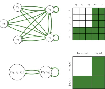
The starting point to build our compression scheme is a well-known combinatorial problem: Find the quotient set of the structural equivalence relation applying to the vertices of a graph. As the resulting equivalence classes form a partition of the vertex set by grouping together vertices with an identical (first-order) structure – that is with identical neighbourhoods – one can exploit such classes to compress the graph representation, as illustrated in Figure 1. Struc-tural equivalence can thus be used for the lossless compression of static graphs, and we later list the improvements one needs in order to generalise this first simple scheme to the lossy compression of link streams.
2.1. Preliminary Notations
Given a set of vertices V = {v1, . . . ,vn}, we mark:
• P(V) the set of all vertex subsets: P(V) = {V ⊆ V}; • P(V) the set of all vertex partitions:
P(V) = {{V1, . . . ,Vm} ⊆ P(V) : ∪iVi=V ∧ ∀i , j, Vi∩ Vj=∅};
• Given a vertex v ∈ V and a vertex partition V ∈ P(V), we mark V(v) the unique vertex subset in V that contains v.
More generally, this article uses a consistent system of capitalization and typefaces to properly formalise the compression problem and its solution space:
• Vertices are designated by lowercase letters: v, v′ , u, u′; • Vertex sets and vertex subsets by uppercase letters: V, V, V′;
• Vertex partitions and sets of vertex subsets by calligraphic letters: V, V′
, P(V), H (V), I(V); • Sets of vertex partitions by Gothic letters: P(V), H(V), I(V).
v1 v2 v3 v4 v5 v1 v2 v3 v4 v5 v1 v2 v3 v4 v5 {v1,v2,v3} {v4,v5} {v1,v2,v3} {v4,v5} {v5 ,v4 } {v3 ,v2 ,v1 }
Figure 1: Lossless compression of a 5-vertex, 16-edge graph (above) into a 2-vertex, 3-edge graph (below). The adjacency-list representation is given on the left and the adjacency-matrix representation on the right.
2.2. The Lossless GCP
To begin with, we consider a simple case: Directed static graphs, with possible self-loops on the vertices. Definition 1 (Directed Graph).
Adirected graph G = (V, E) is characterised by: • A set of vertices V;
• A set of directed edges E ⊆ V×V.
For all vertex v ∈ V, we respectively mark Nin(v) = {v′ ∈ V : (v′,v) ∈ E} and Nout(v) = {v′ ∈ V : (v, v′) ∈ E} the
in-coming and the out-going neighbourhoods of v.
The upper part of Figure 1 gives an example of directed graph made of |V| = 5 vertices and |E| = 16 edges. It is represented in the form of adjacency lists (on the left), where each edge is represented as an arrow going from a source vertex v ∈ V to a target vertex v′∈ V, as well as in the form of an adjacency matrix (on the right), where edges are represented within a binary matrix of size |V| × |V|.
The combinatorial problem we now formalise builds on the classical relation of structural equivalence applying to the vertex set of a graph [16].
Definition 2 (Structural Equivalence).
Thestructural equivalence relation ∼ ⊆ V2 is defined on directed graphs by the equality of neighbourhoods: Two vertices(v, v′) ∈ V2arestructurally equivalent if and only if they are connected to the same vertices. Formally:
v ∼ v′ ⇔ Nin(v) = Nin(v′) and Nout(v) = Nout(v′).
A vertex subset V ∈ P(V) is structurally consistent if and only if all its vertices are structurally equivalent with each others, and a vertex partition V ∈ P(V) is structurally consistent if and only if all its vertex subsets are struc-turally consistent. We respectively mark eP(V) and eP(V) the sets of structurally-consistent vertex subsets and vertex partitions:
V ∈ eP(V) ⇔ ∀(v, v′
) ∈ V2, v ∼ v′. V ∈ eP(V) ⇔ ∀V ∈ V, V ∈ eP(V).
The lower part of Figure 1 uses the fact that v1 ∼ v2 ∼ v3and that v4 ∼ v5to define a structurally-consistent vertex partition V = {V1,V2} made of two structurally-consistent vertex subsets V1={v1,v2,v3} and V2={v4,v5}.
Because all vertices belonging to a structurally-consistent vertex subset have the exact same neighbourhoods, one can use this structural redundancy to simplify the graph representation. Such a compression first consists in aggregat-ing all vertices in structurally-consistent subsets to form compressed vertices, then in aggregataggregat-ing all edges between couples of structurally-consistent subsets to form compressed edges. The resulting compressed graph provides a smaller, yet complete description of the initial one.
Definition 3 (Compressed Directed Graph).
Given a directed graph G =(V, E) and a structurally-consistent vertex partition V ∈ eP(V), the compressed directed graph V(G) = (V, E) is the graph such that:
• V is the set of (compressed) vertices;
• E ⊆ V×V is the set of (compressed) directed edges such that:
∀(V, V′) ∈ V×V, (V, V′) ∈ E ⇔ ∀v ∈ V, ∀v ′
∈ V′,(v, v′) ∈ E ⇔ ∃v ∈ V, ∃v′∈ V′,(v, v′) ∈ E. Note that both conditions are equivalent since V and V′are structurally consistent.
The lower part of Figure 1 shows the effect of such a compression on the graph’s representations. Regarding adjacency lists, no more than one compressed edge is encoded between two given compressed vertices. Regarding the adjacency matrix, cells are merged into “rectangular tiles” containing only one binary value for each couple of compressed ver-tices.
These definitions lead to a well-known combinatorial problem that we call here the Lossless Graph Compression Problem(Lossless GCP). It simply consists in finding the quotient set of the structural equivalence relation, that is the smallest structurally-consistent partition of V.
Definition 4 (The Lossless Graph Compression Problem).
Given a directed graph G =(V, E), find a structurally-consistent vertex partition V∗∈ eP(V) with minimal size |V∗|: V∗ = arg min
V∈eP(V) |V|.
In Figure 1, the represented structurally-consistent vertex partition is the smallest: One cannot find such another partition that contains fewer vertex subsets. This is hence the most optimal lossless compression of the graph.
2.3. Related Problems
Note that structural equivalence is the stricter form of vertex equivalence one might consider for graph analy-sis [20, 21]. Yet, other equivalence relations are traditionally used in the literature in social sciences for the detection of other kinds of structural patterns, such as automorphic equivalence (two vertices are equivalent if there is an iso-morphic graph such that these vertices are interchanged) and regular equivalence [13] (two vertices are equivalent if they are equally related to other equivalent classes). Because these two latter equivalence relations are less strict, they induce smaller vertex partitions with bigger classes. But more importantly, and contrary to structural equivalence, the resulting compression scheme is not reversible in the sense that one cannot find back the initial graph from the equivalent classes and their compressed edges.
Structural equivalence, and so the GCP, is also related to community detection [22], also known as graph clus-tering, that is a classical problem for graph analysis which consists in finding groups of vertices that are strongly connected with each others while being loosely connected to other groups. However, dense and isolated clusters are only particular examples of structurally-consistent classes. They correspond to dense diagonal blocks in the adjacency matrix. The notion of structural equivalence is more generally interested in groups of vertices with similar relational
patterns, that is in any block of equal-density within the adjacency matrix (not necessarily dense and not necessarily on the diagonal, as in other work focusing on block compression [6, 2, 3]). Hence, the GCP is more strongly related to the family of edge compression techniques [8] such as modular decomposition1[3], matching neighbours, and power
graph analysis[9]. In the latter, one is searching for groups of vertices that have similar relation patterns of any sort. Because it is more generally interested in the compression of equal-density blocks, the GCP can lastly be seen as a strict instance of block modelling [16, 20, 13, 15], another classical method of network analysis that relies on structural equivalence to discover roles and positions in social networks.
2.4. Possible Generalisations
This first formulation of the GCP is restricted to static simple graphs. Moreover, it only allows lossless com-pression, that is compression of vertices with identical neighbourhoods, which is a quite stringent and unrealistic condition for empirical research. In what follows, we list the requirements to formulate a more general and more flexible optimisation problem allowing for the lossy compression of temporal graphs.
From simple graphs to multigraphs (see 3.1). This first version of the GCP is restricted to simple graphs (no more than one edge between two given vertices). Yet, it is easily generalisable to multigraphs (multiple edges are allowed between two given vertices). Such a generalisation has two advantages. First, multigraphs are strictly more general than simple graphs since simple graphs can be considered as a particular cases of multigraphs. Second, multigraphs are more consistent with the lossy compression scheme later presented since the end result of lossy compression is not necessarily a simple graph (as edges are aggregated into multiedges during compression).
From lossless to lossy compression (see 3.2). This first version of the GCP is lossless in the sense that the result of compression contains all the information that is required to errorlessly build back the initial graph. However, such a lossless compression – relying on exact equivalence – is quite inefficient in the case of real graphs within which identical neighbourhoods are quite unlikely. One hence needs a measure of information loss to allow for a more flexible compression scheme.
From vertex to edge partitions (see 3.3). This first version of the GCP consists in finding an interesting vertex par-titionto compress the graph, thus inducing a partition of its edges. This relates to classical approaches such as modular decompositionwhere subsets of vertices (modules) that have similar neighbourhoods are exploited to compressed the graph’s structure. However, this can be generalised to the direct search for edge partitions, that is the search for interesting edge subsets that do not all necessarily rest on similar vertex subsets. This relates to less known approaches such as power-graph decomposition that allows for a more subtle analysis of the graph’s structure.
Adding constraints to the set of feasible vertex subsets (see 3.4). In this first version of the GCP, one considers any possible vertex subset as a potential candidate for compression, thus leading to an unconstrained compression scheme. However, in order to represent and to preserve additional constraints that might apply on the vertex structure, one might want to only consider “feasible” vertex subsets when searching for an optimal partition. This requires to integrate such additional constraints within the compression scheme.
From static graphs to link streams (see 3.5). Our last generalisation step consists in integrating a temporal dimen-sion within the optimisation problem in order to deal with the compresdimen-sion of link streams. The structural equiv-alence relation hence needs to be redefined with respect to this additional dimension and equivalent classes will then be only valid on given time intervals. In this context, one is hence searching for aggregates that partition the Cartesian product of the vertex set and of the temporal dimension.
3. Generalisation: From Lossless Static Graphs to Lossy Mutlistreams 3.1. From Graphs to Multigraphs
Most approaches in the domain of graph theory focus on the analysis of simple graphs, that is graphs for which at most one edge is allowed between two vertices, thus represented as binary adjacency matrices. This is also the case when it comes to the field of graph compression (see for example [13, 4, 5, 6, 8]). Yet, in the scope of this article, we aim at the compression of multigraphs, that is graphs for which multiple edges are allowed between two vertices, thus represented as integer adjacency matrices. As simple graphs are special cases of multigraphs, the resulting approach is necessarily more general.
In some articles on graph compression, the generalisation to multigraphs would be quite straightforward as the result of compression – that is the compressed graph – already is, in fact, a multigraph (see for example [6]). Even if not explicitly formalised, research perspectives in that direction are sometimes provided [9]. Yet, other approaches natively deals with multigraph compression by directly taking into account, within the compression scheme, the presence of multiple edges [2, 3]. Statistical methods for variable co-clustering also offers compression frameworks that are designed for numerical (non-binary) matrices [23, 15, 14]. This is the approach we choose here by directly working with multigraphs.
Definition 5 (Directed Multigraph).
Adirected multigraph MG = (V, e) is characterised by: • A set of vertices V;
• A multiset of directed edges (V×V, e)
where e : V×V → N is the edge function, that is the multiplicity function counting the number of edges e(v, v′) ∈N going from a given source vertex v ∈ V to a given target vertex v′∈ V.
We also define the additive extension of the edge function on couples of vertex subsets: e: P(V)×P(V) →N such that e(V, V′
) = X
(v,v′)∈V×V′
e(v, v′).
It simply counts the number of edges going from any vertex of a given source subset V ∈ P(V) to any vertex of a given target subset V′∈ P(V). In particular, e(V, V) is the total number of edges in the multigraph, e(V, v) is
the in-coming degree of v and e(v, V) its out-going degree.
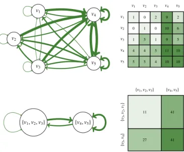
The upper part of Figure 2 gives an example of directed multigraph made of |V| = 5 vertices, that is |V×V| = 25 multiedges, and e(V, V) = 40 edges distributed within V×V. It is represented in the form of adjacency lists (on the left), where each multiedge is represented as an arrow which width is proportional to the number of edges e(v, v′) going from a source vertex v to a target vertex v′, as well as in the form of an adjacency matrix (on the right), where the edge function is represented as an integer matrix of size |V|×|V|.
Structural equivalence could then be generalised to multigraphs in order to define, as done previously for simple graphs, a Lossless Multigraph Compression Problem (MGCP). In few words, the structural equivalence relation would be defined on directed multigraphs by the equality of the edge function: Two vertices are hence structurally equivalent if and only if they are each connected the same number of times to the different graph’s vertices. However, as we are interested in this article in lossy compression, we directly consider an alternative version of the MGCP that relies on a stochastic relaxation of the structural equivalence relation and on an appropriate measure of information loss.
3.2. From Lossless to Lossy Compression
Information-theoretic compression first requires a stochastic model of the data, that is a model of the multigraph to be compressed. The measure of information loss that we present in this subsection has been previously introduced for the aggregation of geographical data [24] and for the summarisation of execution traces of distributed systems [19]. The first contribution of this article in this regard is the application of this measure to graph compression. Moreover, the underlying stochastic models were not made explicit in previous work. Our second contribution is hence the
v1 v2 v3 v4 v5 v1 v2 v3 v4 v5 v1 v2 v3 v4 v5 1 0 2 9 2 0 1 0 10 6 1 5 1 9 5 4 4 5 11 10 5 5 4 10 10 {v1,v2,v3} {v4,v5} {v1,v2,v3} {v4,v5} {v5 ,v4 } {v3 ,v2 ,v1 } 11 41 27 41
Figure 2: Lossy compression of a 5-vertex, 40-edge multigraph (above) into a 2-vertex, 40-edge multigraph (below). In the adjacency-list
repre-sentation(on the left), the width of arrows is proportional to the edge function, that is to the number of edges going from a source vertex to a target vertex.
thorough formalisation of the graph model we use, in order to properly justify and interpret the resulting measure. In few words, we model a multigraph as a set of edges that are stochastically distributed within the two-dimensional set of multiedges V×V: Each edge has a particular location within this space, characterised by its source vertex and its target vertex. The edge function e : V×V →N hence characterises the empirical distribution of the edges within the multigraph, thus allowing to model the data as a discrete random variable (X, X′) taking on V×V.
Definition 6 (Observed Variable).
The observed variable (X, X′) ∈ V×V associated with a multigraph MG = (V, e) is a couple of discrete random
variables having the empirical distribution of edges in MG: Pr((X, X′) = (v, v′)) = e(v, v
′)
e(V, V) def
= p(X,X′)(v, v′).
In other terms, p(X,X′)(v, v′) represents the probability that, if one chooses an edge at random among the e(V, V) edges
of the multigraph, it will go from the source vertex v to the target vertex v′. For example, matrix (i) in Figure 3 represents the distribution of the observed variable associated with the multigraph of Figure 2.
We then define the edge distribution of a multigraph that have been compressed according to a vertex partition V ∈ P(V) by defining a second random variable taking on the multiedge partition V×V ∈ P(V×V).
Definition 7 (Compressed Variable).
The compressed variable V×V(X, X′) ∈ V×V associated with an observed variable (X, X′) ∈ V×V and a vertex partition V ∈ P(V) is the unique couple of vertex subsets in V×V that contains (X, X′):
V×V(X, X′) = (V(X), V(X′)) ∈ V×V.
It hence has the following distribution2:
Pr(V×V(X, X′) = (V, V′)) = e(V, V ′ ) e(V, V) def = pV×V(X,X′)(V, V′).
v1 v2 v3 v4 v5 v1 v2 v3 v4 v5 1 120 1200 1202 1209 1202 0 120 1201 1200 12010 1206 1 120 5 120 1 120 9 120 5 120 4 120 4 120 5 120 11 120 10 120 5 120 5 120 4 120 12010 12010
(i) Observed Variable: (X, X′) ∈ V×V v1 v2 v3 v4 v5 v1 v2 v3 v4 v5
(ii) Vertex Partition: V ∈ P(V) → Multiedge Partition: V×V ∈ P(V×V) {v1,v2,v3} {v4,v5} {v4 ,v5 } {v1 ,v2 ,v3 } 11 120 41 120 27 120 12041
(iii) Compressed Variable: V×V(X, X′) ∈ V×V v1 v2 v3 v4 v5 v1 v2 v3 v4 v5 1 25 1 25 1 25 1 25 1 25 1 25 251 251 251 251 1 25 1 25 1 25 1 25 1 25 1 25 1 25 1 25 1 25 1 25 1 25 1 25 1 25 1 25 1 25
(iv) Uniform External Variable: (Y, Y′) ∈ V×V v1 v2 v3 v4 v5 v1 v2 v3 v4 v5 14 120 17 120 21 120 34 120 34 120 11 120 15 120 12 120 49 120 33 120
(iv’) Degree-preserving External Variable: (Y, Y′) ∈ V×V v1 v2 v3 v4 v5 v1 v2 v3 v4 v5 11 120× 1 9 11 120× 1 9 11 120× 1 9 41 120× 1 6 41 120× 1 6 11 120× 1 9 11 120× 1 9 11 120× 1 9 41 120× 1 6 41 120× 1 6 11 120× 1 9 11 120× 1 9 11 120× 1 9 41 120× 1 6 41 120× 1 6 27 120×16 12027×16 12027×16 12041×14 12041×14 27 120× 1 6 27 120× 1 6 27 120× 1 6 41 120× 1 4 41 120× 1 4 (v) Decompressed Variable: V×V(Y,Y′)(X, X′) ∈ V×V v1 v2 v3 v4 v5 v1 v2 v3 v4 v5 (v’) Decompressed Variable: V×V(Y,Y′)(X, X′) ∈ V×V
(vi) Information Loss: loss(V×V) = DKL(p(X,X′)|| pV×V(Y,Y′ )(X,X′))
Figure 3: Lossy compression consists in (i) modelling the multigraph as a random variable (X, X′) having the empirical distribution of edges in V×V, (ii) choosing a vertex partition V, and so a multiedge partition V×V that is used to compress (X, X′), (iii) computing the distribution of the resulting compressed variable V×V(X, X′) by applying partition V×V onto (X, X′), (iv) taking an external variable (Y, Y′) (for example (iv) uniformly distributed or (iv’) preserving the degree profile of vertices) to project back the distribution of V×V(X, X′) into V×V, (v) computing the distribution
of the resulting decompressed variable V×V(Y,Y′)(X, X′) by first choosing (X, X′), then choosing (Y, Y′) conditioned on V×V(Y, Y′) = V×V(X, X′),
and (vi) comparing the distribution of (X, X′) with the distribution of V×V
(Y,Y′)(X, X′) by using information-theoretic measures such as the entropy
In other terms, pV×V(X,X′)(V, V′) represents the probability that, if one chooses an edge at random among the e(V, V)
edges of the multigraph, it will go from a vertex of the source subset V to a vertex of the target subset V′. For example, matrix (ii) in Figure 3 represents the multiedge partition V×V induced by the vertex partition V = {{v1,v2,v3}, {v4,v5}} and matrix (iii) then represents the distribution of the resulting compressed variable V×V(X, X′).
In order to quantify the information that has been lost during this compression step, we propose to compare the information that is contained in the initial multigraph (that is in the observed variable (X, X′)) with the information that is contained in the compressed multigraph (that is in the compressed variable V×V(X, X′)). To do so, we project back the compressed distribution onto the initial value space V×V by defining a third random variable, the external variable (Y, Y′) ∈ V×V, that models additional information that one might have at his or her disposal when trying to decompress the multigraph. It is hence assumed to have a distribution that is somehow “informative” of the initial distribution. It then induces a fourth variable, the decompressed variable V×V(Y,Y′)(X, X′), that models an approximation of the
initial multigraph inferred from the combined knowledge of the compressed variable V×V(X, X′) and of the external variable (Y, Y′). This last variable is hence defined according to the distribution of the external variable within the multiedge subsets.
Definition 8 (Decompressed Variable).
Thedecompressed variable V×V(Y,Y′)(X, X′) ∈ V×V associated with an observed variable (X, X′) ∈ V×V, a vertex
partition V ∈ P(V), and an external variable (Y, Y′) ∈ V×V, is the result of this external variable (Y, Y′) conditioned by its compression V×V(Y, Y′) being equal to the result of the compressed variable V×V(X, X′):
V×V(Y,Y′)(X, X′) = (Y, Y′) | V×V(Y, Y′) = V×V(X, X′) ∈ V×V.
It hence has the following distribution3: Pr(V×V(Y,Y′)(X, X′) = (v, v′)) = e(V×V(v, v′)) e(V, V) p(Y,Y′)(v, v′) pV×V(Y,Y′)(V×V(v, v′)) def = pV×V(Y,Y′ )(X,X′)(v, v ′ ).
In other terms, pV×V(Y,Y′ )(X,X′)(v, v′) represents the probability that, if one (i) chooses an edge (u, u′) at random among
the e(V, V) edges of the multigraph, (ii) considers its compressed multiedge subset V×V(u, u′) = (V, V′) ∈ V×V, and (iii) chooses a source vertex within V and a target vertex within V′according to the distribution p
(Y,Y′)of the external
variable within this multiedge subset, then one will result with an edge going from the source vertex v to the target vertex v′. For example, matrix (iv) in Figure 3 represents a uniformly-distributed external variable (Y, Y′) ∈ V×V that is used to decompress V×V(X, X′) (see Blind Decompression below). Matrix (iv’) represents another such external
2By applying the law of total probability:
Pr(V×V(X, X′) = (V, V′)) = X (v,v′)∈V×V Pr(V×V(X, X′) = (V, V′) | (X, X′) = (v, v′)) | {z } =1 if (v,v′)∈V×V′,and 0 else Pr((X, X′) = (v, v′)) = X (v,v′)∈V×V′ Pr((X, X′) = (v, v′)) = X (v,v′)∈V×V′ e(v, v′) e(V, V) = e(V, V′) e(V, V)
Note that, more generally, compression could be defined for any (possibly stochastic) function of the observed variable (X, X′), thus modelling what
is sometimes called a “soft partitioning” of the vertices. The information-theoretic framework presented in this article, along with all the measures it contains, are straightforwardly generalisable to such setting. However, because it is often much easier to interpret the result of compression when it is based on “hard partitioning”, especially in the case of vertex partitioning, we focus in this article on this simpler setting.
3By applying the law of total probability:
Pr(V×V(Y,Y′)(X, X′) = (v, v′)) = Pr((Y, Y′) = (v, v′) | V×V(Y, Y′) = V×V(X, X′))
= X (V,V′)∈V×V Pr((Y, Y′) = (v, v′) | V×V(Y, Y′) = (V, V′)) | {z } =0 if (V,V′) , V×V(v,v′) Pr(V×V(X, X′) = (V, V′)) = Pr((Y, Y′) = (v, v′) | V×V(Y, Y′) = V×V(v, v′)) Pr(V×V(X, X′) = V×V(v, v′)) = Pr((Y, Y ′) = (v, v′)) Pr(V×V(Y, Y′) = V×V(v, v′)) e(V×V(v, v′)) e(V, V) .
variable (see Degree-preserving Decompression below). Matrices (v) and (v’) then represent the distribution of the resulting uniformly decompressed variable V×V(Y,Y′)(X, X′).
Blind Decompression. When the external variable (Y, Y′) is uniformly distributed on V×V, the decompression step is done without any additional information about the initial edge distribution:
p(Y,Y′)(v, v′) = 1 |V×V| ⇒ pV×V(Y,Y′ )(X,X′)(v, v ′ ) = e(V×V(v, v ′)) e(V, V) 1 |V×V(v, v′)|.
In this case, only the knowledge of the compressed variable hence is exploited. The decompressed variable is hence the result of a uniform trial among the multiedges contained in V×V(X, X′), that is a “maximum-entropy sampling” guarantying that no additional information has been injected during decompression.
Reversible Decompression. To the contrary, when the external variable (Y, Y′) has the same distribution than the observed variable (X, X′), then the decompression step is done with a full knowledge of the initial edge distribution:
p(Y,Y′)(v, v′) = p(X,X′)(v, v′) ⇒ V×V(Y,Y′)(X, X′)(v, v′) =
e(v, v′)
e(V, V) = p(X,X′)(v, v ′
).
In this case, the decompressed variable also has the same distribution than the observed variable, meaning that one fully restores the initial multigraph when decompressing.
Degree-preserving Decompression. An intermediary example of external information can be derived from the knowl-edge of the vertex degrees in the initial multigraph:
p(Y,Y′)(v, v′) = pX(v) pX′(v′) = e(v, V) e(V, V) e(V, v′) e(V, V) ⇒ pV×V(Y,Y′ )(X,X′)(v, v ′ ) = e(V×V(v, v ′ )) e(V, V) e(v, V) e(V, v′) e(V(v), V) e(V, V(v′)). In this case, the decompression step takes into account the initial vertex degrees and the resulting multigraph hence has the same degree profile than the initial one. The corresponding generative model is hence similar to the one of a configuration model[25]: Multigraphs are sampled according to the compressed variable, while also preserving the initial degree profile.
Now that we have defined compression and decompression as sequential operations on stochastic variables, we exploit a classical measure of information theory to quantify the information that is lost during such a process. In-tuitively, it consists in comparing the initial edge distribution (the one of the observed variable (X, X′)) with the approximated edge distribution (the one of the decompressed variable V×V(Y,Y′)(X, X′)). In this article, we propose to
do so by using the relative entropy of these two distributions – also known as the Kullback-Leibler divergence [26, 27] – as it is the most canonical measure of dissimilarity provided by information theory to compare an approximated probability distribution to a real one.
Definition 9 (Information Loss).
Theinformation loss induced by a vertex partition V ∈ P(V) on an observed variable (X, X′) ∈ V×V, and according to an external variable(Y, Y′) ∈ V×V, is given by the entropy of (X, X′) relative to V×V(Y,Y′)(X, X′):
loss(V×V) = X (v,v′)∈V×V p(X,X′)(v, v′) log2 p(X,X′)(v, v′) pV×V(Y,Y′ )(X,X′)(v, v′) ! = X (v,v′)∈V×V e(v, v′) e(V, V)log2 e(v, v′) e(V×V(v, v′)) p(Y,Y′)(v, v′) pV×V(Y,Y′)(V×V(v, v′)) !
Note that information loss isadditively decomposable. It can be expressed as a sum of information losses defined at the subset level instead of at the partition level:
loss(V×V) = X (V,V′)∈V×V
loss(V, V′) with loss(V, V′) = X (v,v′)∈V×V′ e(v, v′) e(V, V)log2 e(v, v′) e(V, V′) p(Y,Y′)(v, v′) pV×V(Y,Y′)(V, V′) ! .
Intuitively, this measure considers the following reconstruction task: Imagine that all the edges of a multigraph have been “detached” from their vertices and put into a bag. An observer is now taking one edge out of the bag and tries to guess its initial location, that is its source and target vertices. We then compare two peoples trying to do so: One having a perfect knowledge of the distribution p(X,X′) of the edges in the initial multigraph (e.g., matrix (i) in Figure 3); The
second only having an approximation pV×V(Y,Y′ )(X,X′) of this distribution, obtained through the compression, then the
decompression of the initial distribution (e.g., matrices (v) and (v’) in Figure 3). Relative entropy then measures the average quantity of additional information (in bits per edge) that the second observer needs in order to make a guess that is as informed as the guess of the first observer. In other words, relative entropy quantifies the information that has been lost during compression, that is no longer contained in the compressed graph, and that cannot be retrieved from the knowledge of the external variable.
Blind Decompression. When the external variable is uniformly distributed on V×V, relative entropy simply quantifies the information that has been lost during compression, without the help of any additional information:
p(Y,Y′)(v, v′) = 1 |V×V| ⇒ loss(V, V ′ ) = X vv∈V×V′ e(v, v′) e(V, V)log2 e(v, v′) e(V, V′)|V×V ′| ! .
Reversible Decompression. When the external variable (Y, Y′) has the same distribution than the observed variable (X, X′), compression then induces no information loss – whatever the chosen vertex partition V – since all the infor-mation required to reconstruct the initial multigraph is reinjected during the decompression step:
p(Y,Y′)(v, v′) = p(X,X′)(v, v′) ⇒ loss(V, V′) = 0.
Degree-preserving Decompression. In this intermediary context, relative entropy quantifies the information that has been lost during compression, and that cannot be retrieved from the additional knowledge of the vertex degrees in the initial multigraph: p(Y,Y′)(v, v′) = pX(v) pX′(v′) = e(v, V) e(V, V) e(V, v′) e(V, V) ⇒ loss(V, V′) = X (v,v′)∈V×V′ e(v, v′) e(V, V)log2 e(v, v′) e(V, V′) e(v, V) e(V, v′ ) e(V, V) e(V, V′) ! .
Related Measures. Relative entropy is one among many measures that can be found in the literature to quantify information loss in graph compression. Given an initial multigraph and a decompressed one, which is described by the approximated edge distribution, any measure of weighted graph similarity may be relevant to quantify the impact of compression [1]: E.g., the percentage of edges in common, the size of the maximum common subgraph or of the minimum common supergraph, the edit distance, that is the insertion and removal of vertices and edges needed to
go from one graph to another [28], or any measure aggregating the similarities of vertices from graph to graph (e.g., Jaccard index, Pearson coefficient, cosine similarity on vertex neighbourhoods).
More sophisticated graph-theoretical measures go beyond the mere level of edges by taking into account paths within the two compared graphs [2]: “[T]he best path between any two nodes should be approximately equally good in the compressed graph as in the original graph, but the path does not have to be the same.” More generally, query-based measures aim at quantifying the impact of compression on the results of goal-oriented queries regarding the graph structure: E.g., queries about shortest paths, about degrees and adjacency, about centrality and community structures (see for example [29, 30, 31]). The expected difference between the results of queries on the initial graph and the results of queries on the decompressed graph thus provides a reconstruction error that serves as a goal-oriented information loss [6]. To some extent, we are interested in this article in adjacency-oriented queries, that is the most canonical ones, taking the perspective of the weighted adjacency matrices of the two compared graphs: What is the weight of the multiedge located between two given vertices of the initial multigraph? Relative entropy measures the expected error when answering this query from the only knowledge of the compressed graph.
More generally, this perspective is related to the density profile of edges within the graph. Hence, density-based measures [5] seems more relevant than other traditional connectivity measures: E.g., the Euclidean distance or the mean squared error between the two density matrices [2, 3], the average variance within matrix blocks [13], and many other measures inherited from traditional block modelling methods [20]. Note that, when it comes to the latter, the stochastic model underlying our compression framework is similar, but not equivalent to the one of block modelling. The compressed matrix describes in our case the parameters of a multinomial distribution from which the graph’s edges are sampled, whereas it describes in the case of block modelling the parameters of |V×V| independent Bernouilli distributions. In other words, our model gives the probability that an edge – taken at random – is located between two given vertices, and not the probability that an edge exists between two given vertices (see for example block model compression in [6]).
Because of this particular stochastic model, we chose in this article an information-theoretic approach to measure information loss. This allows to derive a measure that is clearly in line with the defined model and which can be easily interpreted within the realm of information theory. Among tools provided by this theory, other approaches use the principles of minimum description length [4, 6] to compress a graph using the density-based model in an optimal fashion. In the same line of thinking, traditional tools for Bayesian inference propose to interpret the compressed graph as a generative model and the initial graph as observed data, then computes the likelihood of the data given the model as a measure of information loss [15]. A similar Bayesian interpretation of relative entropy could be given, as it measures the difference of likelihood between two generative models of the multigraph: One corresponding to e(V, V) independent trials with the empirical distribution of the multigraph’s edges; The second corresponding to e(V, V) independent trials with the distribution obtained through compression, and then decompression. Similarly, co-clustering[23] interprets the graph’s adjacency matrix as the joint probability distribution of two random variables, then finds two vertex partitions that minimise the loss in mutual information between these two variables [27] from the initial graph to the compressed graph. This is shown to be equivalent to minimising the relative entropy between the initial distribution and a decompressed distribution that preserves the marginal values. It is hence equivalent to our measure of information loss in the particular case of a decompression scheme that takes into account additional information regarding the vertex degrees.
3.3. From Vertex to Edge Partitions
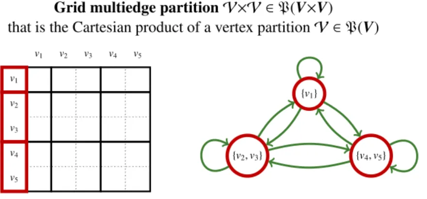
By providing a measure of information loss, previous subsection focuses on the objective function of the GCP, that is on the quality measure to be optimised. We now focus on the solution space of this problem, that is the set of partitions that one actually consider for compression. The original GCP presented in Section 2 consists in using a vertex partition V ∈ P(V) to then determine a multiedge “grid” partition (see top-left matrix of Figure 4):
V×V = {V×V′ : V ∈ V ∧ V′∈ V} ∈ P(V×V),
such that two multiedges (v, v′) and (u, u′) are in the same multiedge subset V×V′if and only if their source vertices are both in V and their target vertices are both in V′:
Grid multiedge partition V×V ∈ P(V×V)
that is the Cartesian product of a vertex partition V ∈ P(V)
v1 v2 v3 v4 v5 v1 v2 v3 v4 v5 {v1} {v2,v3} {v4,v5}
Cartesian multiedge partition VV ∈ P
×(V×V)
consisting in Cartesian multiedge subsets V×V
′∈ P(V×V)
v1 v2 v3 v4 v5 v1 v2 v3 v4 v5 {v4} {v1,v2} {v3,v5}Figure 4: Two partitioning schemes that one might consider to define the solution space of the GCP. Multiedge subsets are represented with hatching when they are not “compact tiles”.
In other terms, the induced two-dimensional partitioning of the multiedge set V×V is the Cartesian product of a one-dimensional partitioning of the vertex set V. This first compression scheme is classically used in macroscopic graph models such as block models and community-based representations. One of the reason is that the result of compression can still be represented as a graph, which vertices are the subsets of the vertex partition and which multiedges are the subsets of the multiedge “grid” partition (see top-right graph of Figure 4)
However, this results in a quite constrained solution space for the optimisation problem: Only a small number of partitions of V×V are actually feasible. One might instead consider a less constrained solution space by allowing a larger number of multiedge partitions to be used for compression, by for example considering partitions of the multiedge set V×V that are made of Cartesian products of two vertex subsets V×V′⊆ P(V×V).
Definition 10 (Cartesian Multiedge Partitions).
Given a vertex set V, the set of Cartesian multiedge partitions P×(V×V) ⊂ P(V×V) is the set of multiedge partitions that are made of Cartesian products of vertex subsets4:
P×(V×V) = {{(V1× V1′), . . . , (Vm× Vm′)} ⊆ P(V)×P(V)
: ∪i(Vi× Vi′) = V×V ∧ ∀i , j, (Vi× Vi′) ∩ (Vj× V′j) = ∅}.
Such Cartesian partitions of V×V hence contains “rectangular” multiedge subsets5 (see bottom-left matrix of Fig-ure 4). Hence, although the result of compression can no longer be represented as a graph, it can be represented as
4There is an abuse of notation in this definition when writing that “V×V′∈ P(V)×P(V)”. We should instead write that “V×V′∈ P(V×V) such
that (V, V′) ∈ P(V)×P(V)”, but we prefer the former for notation conciseness.
5Note that each of these multiedge subsets is indeed a rectangle in the adjacency matrix, modulo a reordering of its rows and columns. It might
a directed hypergraph – or as a power graph [8, 9] – that is a graph where edges can join couples of vertex subsets instead of couples of vertices (see bottom-right graph of Figure 4).
Related Work. Most classical approaches for graph compression are based on the discovery of vertex partitions. This is for example the case of most work on graph summarisation [5, 6], block modelling [13], community detection [22], and modular decomposition [3]. As previously said, one of the interests of such vertex partitioning is that the result of compression is still a graph (a set of compressed vertices connected by a set of compressed edges) that can hence be represented, analysed, and visualised with traditional tools [4, 2]. However, the number and diversity of feasible solutions – that is the set of vertex partitions – is quite limited when compated to the full space of matrix partitions.
As proposed above, some approaches hence focus on edge partitions, instead of vertex partitions, in order to provide more expressive compression schemes, but only on particular edge partitions, in order to preserve some fundamental structures of graph data. The most generic framework is formalised by power graph analysis [8, 9] and Mondrian processes [32], where edge subsets are only required to be the Cartesian product of vertex subsets. Such edge subsets can hence be represented as compressed edges between couples of compressed vertices. But since different edge subsets can lead to overlapping vertex subsets, the resulting compressed graph is no longer a graph, but an hypergraph (or a power graph). While still interpretable within the broad realm of graph theory, power graphs are more expressive [2] than classical approaches – such as community partitions – since a given vertex might belong to different similarity groups: It might be similar to a given group of vertices with respect to a given part of the graph, and similar to another group of vertices with respect to another part (see examples in [9]).
3.4. Adding Constraints to the Set of Feasible Vertex Subsets
A wide variety of approaches span from generic edge partitions to more constrained schemes that “impose restric-tions on the nature of overlap” for example by “fixing the topology of connectivity between overlapping nodes” [9] such as in clique percolation, spin models, mixed-membership block models, latent attribute models, spectral cluster-ing, and link communities. This aims at expressing particular topological properties within the compression scheme in order to produce meaningful graphs with respect to some particular analysis framework. “Frequent patterns possibly reflect some semantic structures of the domain and therefore are useful candidates for replacement” [1].
In the partitioning scheme hereabove presented, the Cartesian product of any two vertex subsets (V, V′) ∈ P(V)×P(V) gives a feasible multiedge subset V×V′∈ P(V×V). In other terms, the solution space is only limited by this Cartesian principle and by the partitioning constraints (covering and non-overlapping subsets). However, one can also con-trol the shape of feasible partitions by directly specifying the feasible vertex subsets that can be combined to build the “rectangular” multiedge subsets of the Cartesian partition. Such additional constraints might prove to be useful to incorporate domain knowledge about particular vertex structures within the compression scheme: By driving the process, feasibility constraints might indeed facilitate the interpretation of the compression’s result according to the expert domain.
Definition 11 (Feasible Multiedge Partitions).
Given a set of feasible vertex subsets ˆP(V) ⊆ P(V), the set of feasible Cartesian multiedge partitions ˆP×(V×V) ⊆ P×(V×V) is the set of Cartesian multiedge partitions which multiedge subsets are only made of feasible vertex subsets:
ˆ
P×(V×V) = {{(V1×V′1), . . . , (Vm×Vm′)} ∈ ˆP(V)× ˆP(V)
: ∪i(Vi×Vi′) = V×V ∧ ∀i , j, (Vi×Vi′) ∩ (Vj×V′j) = ∅}.
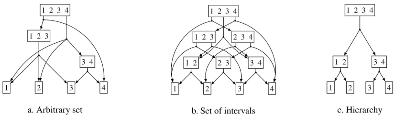
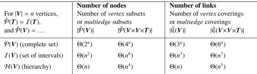
In the most general case, the set of feasible vertex subsets ˆP(V) can be composed of all vertex subset in P(V). However, one can use more constrained – and hence more meaningful vertex structures – to drive the compression scheme and its possible applications. A survey about the types of constraints that have been used in many different domains can be found in [33]. We present below some of these structures and their basic combinatorics.
The Complete Case. When no additional constraint applies to vertex subsets, then: ˆ
Such scheme can be used when no additional useful structure is known about the vertex set, for example to model coalition structuresin multi-agent systems when assuming that every possible group of agents is an adequate candi-date to constitute a coalition [34, 35]. It has been shown that, in this case, the number of feasible partitions grows considerably faster than the number of feasible subsets [36]:
|P(V)| = 2n
and |P(V)| = ω(nn/2 ), where n = |V| is the number of vertices in the graph.
Hierarchies of Vertex Subsets. A hierarchy ˆP(V) = H (V) is such that any two feasible vertex subsets are either disjoint, or one is included in the other:
∀(V1,V2) ∈ H (V)2, V1∩ V2=∅ ∨ V1 ⊆ V2 ∨ V2⊆ V1.
We mark ˆP(V) = H(V) the resulting set of feasible vertex partitions. Such vertex hierarchies can be used to model graphs that are known to have a multilevel nested structure that one wants to preserve during compression. This might include, among others, a community structure that have been preliminarily identified through a hierarchical community detection algorithm [37], a sequence of geographical nested partitions of the world’s territorial units [24]; a hierarchical communication network in distributed computers [19].
It has been shown that the number of feasible subsets in a hierarchy is asymptotically bounded from above by the number of objects it contains [33]: |H (V)| = O(n). The resulting number of feasible partitions however depends on the number of levels and branches in the hierarchy. For a complete binary tree, it is asymptotically bounded by an exponential function: |H(V)| = Θ(αn), with α ≈ 1.226 [38]. Similar results have been found for complete ternary trees
(with α ≈ 1.084 [39]), complete quaternary trees, and so on. Henceforth, for any bounded number of children per node in the hierarchy, the number of feasible partitions exponentially grows with the number of objects.
Sets of Vertex Intervals. Any total order < on the vertex set V induces a set of vertex intervals ˆP(V) = I(V) defined as follows:
I(V) = {[v1,v2] : (v1,v2) ∈ V2} where [v1,v2] = {v ∈ V : v1≤ v ≤ v2}.
We mark ˆP(V) = I(V) the resulting set of feasible vertex partitions. It can be represented as a “pyramid of inter-vals” [33] and such partitions are sometimes called consecutive partitions [40]. Such sets of intervals naturally apply to vertices having a temporal feature (e.g., events, dates, or time periods are naturally ordered by the “arrow of time”) and have hence been exploited for the aggregation of time series [41, 42, 24]. They might also model unidimensional spacial features, such as the geographical ordering of cities on a coast, or on a transport route [43].
The number of intervals of an ordered set of size n is |I(V)| = n(n+1)2 . The resulting number of feasible partitions is |I(V)| = 2n−1[33].
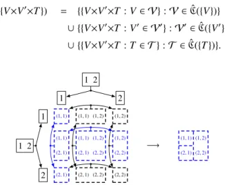
3.5. From Multigraphs to Multistreams
The last step of our generalisation work regards the integration of a temporal dimension within our framework in order to finally deal with the compression of temporal graphs [10]. As argued in the introduction of this article, we build on the link stream representation of such graphs [11, 12]. However, because we also want to deal with cases for which multiple edges are allowed between two vertices at a given time instance, we actually generalise from streams to multistreams, as we did in Subsection 3.1 to generalise from graphs to multigraphs.
Definition 12 (Directed Multistream).
Adirected multistream MS = (V, T, e) is characterised by: • A set of vertices V;
• A set of time instances T ⊆R;
• A multiset of directed edges (V×V×T, e)
where e : V×V×T → N is the edge function, that is the multiplicity function counting the number of edges e(v, v′,t) ∈ N going from a given source vertex v ∈ V to a given target vertex v′ ∈ V at a given time instance t ∈ T.
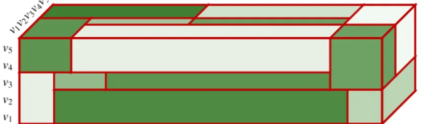
v1 v2 v3 v4 v5 v1v2 v3v4 v5
Figure 5: Multistream compression, that is the Cartesian partitioning of V×V×T, consists in the natural tridimensional generalisation of multigraph compression, that is the Cartesian partitioning of V×V.
In this context, the edge function counts the number of interactions happening between vertices at a given time: e(v, v′,t) is the number of edges going from source vertex v to target vertex v′at time t.
As illustrated in Figure 5, this formalism constitutes an elegant solution to generalise our compression scheme since it simply adds a third dimension T ⊆R to the multigraph’s definition. The GCP is then generalised to this three-dimensional formalism by (i) defining a set of feasible time subsets that preserves the ordering of time instances, that is a set of intervals ˆP(T) = I(T) (see previous subsection), (ii) considering three-dimensional Cartesian multiedge subsets V×V′×T ∈ ˆP(V)× ˆP(V)×I(T), and (iii) computing the information loss on this generalised space in a similar fashion than for the static version of the compression problem. Here is the resulting generalisation in details.
se e D efi n it io n 5 • Time instances: t ∈ T ⊆R; • Time subsets: T ∈ P(T); • Multiedges: (v, v′,t) ∈ V×V×T; • Edge function: e: V×V×T→N; • Compressed edge function:
e: P(V)×P(V)×P(T)→N with e(V, V′ ,T) = X (v,v′)∈V×V′ Z t∈T e(v, v′,t)dt; se e D ef . 1 1
• Feasible time subsets, that is time intervals:T =[t1,t2] ∈ ˆP(T) = I(T) ⊂ P(T); • Feasible multiedge subsets: V×V′×T ∈ ˆP(V)× ˆP(V)×I(T) ⊂ P(V×V×T
); se e D ef . 1 0
• Feasible Cartesian multiedge partitions:
VVT ∈ ˆP×(V×V×T) = {{(V1×V1′×T1), . . . , (Vm×Vm′×Tm)} ∈ ˆP(V)× ˆP(V)×I(T) : ∪i(Vi×Vi′×Ti) = V×V×T∧ (Vi×Vi′×Ti) ∩ (Vj×V′j×Tj) = ∅}; se e D efi n it io n 6 • Observed variable: (X, X′,X′′) ∈ V×V×T with f(X,X′,X′′)(v, v′,t) = e(v, v′,t) e(V, V,T);