HAL Id: hal-03191884
https://hal.umontpellier.fr/hal-03191884
Submitted on 8 Apr 2021HAL is a multi-disciplinary open access archive for the deposit and dissemination of sci-entific research documents, whether they are pub-lished or not. The documents may come from teaching and research institutions in France or abroad, or from public or private research centers.
L’archive ouverte pluridisciplinaire HAL, est destinée au dépôt et à la diffusion de documents scientifiques de niveau recherche, publiés ou non, émanant des établissements d’enseignement et de recherche français ou étrangers, des laboratoires publics ou privés.
SEraMic: a semi-automatic method for the
segmentation of grain boundaries
Renaud Podor, X. Le Goff, J. Lautru, H.P. Brau, M. Massonnet, Nicolas
Clavier
To cite this version:
Renaud Podor, X. Le Goff, J. Lautru, H.P. Brau, M. Massonnet, et al.. SEraMic: a semi-automatic method for the segmentation of grain boundaries. Journal of the European Ceramic Society, Elsevier, In press, �10.1016/j.jeurceramsoc.2021.03.062�. �hal-03191884�
1
SEraMic: a semi-automatic method for the segmentation of grain boundaries
R. Podor*, X. Le Goff, J. Lautru, H.P. Brau, M. Massonnet, N. Clavier
ICSM, Univ Montpellier, CNRS, ENSCM, CEA, Marcoule, France
*Corresponding author
Abstract
The SEraMic method, implemented in the SEraMic plugin for Fiji or ImageJ software, was developed to calculate a segmented image of a ceramic cross section that shows the grain boundaries. This method was used to accurately and automatically determine grain boundary positions and further assess the grain size distribution of monophasic ceramics, metals, and alloys. The only required sample preparation is polishing the cross section to a mirror-like finish. The SEraMic method is based on at least six backscattered electron scanning electron microscopy images of a unique region of interest with various tilt angles ranging from -5° to +5°, which emphasises the orientation contrasts of the grains. Because the orientation contrast varies with the incident beam angle on the sample, the set of images contains information related to all the grain boundaries. The SEraMic plugin automatically calculates and builds a segmented image of the grain boundaries from the set of tilted images. The SEraMic method was compared with classical thermal etching methods, and it was applied to determine the grain boundaries in various types of materials (oxides, phosphates, carbides, and alloys). The method remains easy to use and accurate when the average grain diameter is greater than or equal to 0.25 µm.
Keywords
2 Introduction
The properties of ceramics are closely related to their microstructure (e.g. grain size, amount and distribution of porosity, and chemical homogeneity). Thus, measuring the grain size in a ceramic
(ceramography) is an essential step in the characterisation of its microstructure [1]. To assess the grain size distribution and evaluate the average grain size, it is necessary to collect images with sufficient contrast at the grain boundaries so that they can be segmented, allowing the determination of the position of the grain contours. Recording images that contain the information of the grain boundary position is critical and often difficult to achieve, particularly when the grain size is around or even below the micrometre scale. It requires the use of techniques that aim to create a contrast between the grains, which can be difficult and/or time consuming to implement. Two main families of methods are generally used.
First, grain boundaries can be revealed to create a contrast between the grains. This is achieved by polishing the surface to the mirror grade and then applying either chemical or thermal etching. Images of the material surface are further obtained using optical or scanning electron microscopy. Both methods require either the use of hazardous chemicals [2] or long heat treatments that often have to be optimised when working with new materials [3]. Finally, thermal etching could bias the measurements of grain sizes, particularly when grain growth, surface modifications [4,5,6,7], and/or secondary phase precipitation at the grain boundaries [8] occur during the heat treatment.
As an alternative, a thin section (approximately 30 µm thick) can be cut from the ceramic. The images of the grains are then recorded using optical microscopy in the polarised transmitted light mode. Heilbronner [9] developed an original process, called the Lazy Grain Boundary method, which is based on sets of polarised micrographs or orientation images. This method allows fast and automatic/semi-automatic detection of grain boundaries but has only been used for the study of geological samples using optical microscopy.
Furthermore, methods based on the recording of electron backscatter diffraction (EBSD) maps are under development [10,11,12]. The primary benefit of grain size measurement using EBSD over imaging of etched surfaces is that grain boundaries can be precisely identified owing to contrast modification due to the crystallographic orientation.
3 These different methods are limited by the sample preparation, resolution of the microscope, and/or availability of an EBSD detector. Finally, these techniques can be very expensive in terms of the time required for sample preparation.
Once the images are recorded, the next step relies on image processing and segmentation. Numerous methods currently under development are based on numerical calculations [13,14,15] or deep learning methods [16,17,18]. Finally, several methods can be used to measure the grain size [19], including the intercept method [20,21] and standardised methods, such as planimetric grain size measurement [22]. A set of several hundreds of grains (typically 500–1000) is generally considered to statistically account for the grain size distribution in the material.
In the present study, we propose the development of a reliable, fast, and easy-to-implement method for revealing grain boundaries. This method was tested on various ceramics and alloys. An evaluation criterion of the method is defined to compare the quality of the segmented image obtained while varying the image processing parameters. The image processing associated with this method was implemented in the dedicated ‘SEraMic’ plugin for ImageJ [23] and Fiji [24], which allows fast
segmentation of the grain boundaries in ceramics.
Materials and methods Materials
Five different ceramics and one alloy were used in the present study: (U1-xCex)O2, SnO2, NdPO4, TiC,
YAG, and Ni25Cr. These samples were chosen because they belong to different families of materials, i.e. oxides, phosphates, carbides, and a Ni25Cr alloy.
Five (U1-xCex)O2 oxides were sintered between 1300 and 1600 °C for 1 to 10 h under an Ar/H2
atmosphere to obtain high-density ceramics with different grain sizes. These ceramics are electronic conductors and can be directly observed under high-vacuum conditions.
A SnO2:0.5%CoO ceramic was sintered at 1300 °C for 96 h in air [25]. This ceramic is insulating.
This is denoted as SnO2 in the text.
NdPO4 was sintered at 1400 °C for 4 h [26]. This ceramic is insulating.
TiC was sintered at 1700 °C by spark plasma sintering for 5 min at P = 75 MPa [27]. This ceramic is an electronic conductor.
4 The Ni25Cr (wt.%) alloy was prepared by high-frequency melting from bulk elements with
purities higher than 99.95% [28].
Four yttrium aluminium garnet transparent ceramics (YAG) were provided by IrCer, University of Limoges (France). They were prepared to have different average grain diameters. These ceramics are insulating.
Sample preparation
The TiC and SnO2 pellets were embedded in a resin. All the samples were polished to obtain a
mirror-like surface. After a pre-polishing step performed with SiC papers of various grades, a two-step finishing polish was performed using a 1 µm diamond suspension for 2 min, followed by a 100 nm colloidal silica suspension for 15 min.
Scanning electron microscopy
An environmental scanning electron microscope (SEM, Quanta 200 ESEM FEG, FEI) was used to record the images. The internal ring of a directional backscattered electron (BSE) detector (DBS, FEI) was used to enhance the grain orientation contrast [29]. This detector allows the recording of BSE images at a low acceleration voltage. It can be used under high-vacuum as well as low-vacuum conditions. The magnifications of the SEM were calibrated prior to image recording (see Supplementary File S1). With this calibration step, the measurement errors are limited, and the SEM can be used as an accurate measurement tool [30].
Description of the SEraMic method Principle of the SEraMic method
The method is based on the recording of SEM images using the BSE mode. The image contrast can contain information related to the crystallographic orientation of the grains in the ceramic. These contrasts are related to the variation in the number of BSEs as a function of the crystallographic orientation of the grain relative to the incident electron beam. This mode of contrast (also called channelling contrast) makes it possible to highlight misorientations between grains of identical chemical
5 nature as well as twinning in the grains. These contrasts are at the origin of the eCHORD (electron
CHanneling ORientation Determination) method recently developed by Lafond et al., which aims to obtain orientation maps of polycrystalline materials using a conventional SEM [31].
When recording channelling contrast images, two neighbouring grains with different
crystallographic orientations can exhibit the same grey level (i.e. the same contrast). Thus, they can be identified as a single grain in the image. To overcome this bias, it is possible to modify the contrast between these two grains by changing the incidence angle of the primary electron beam with respect to the surface of the material. This can be easily achieved by tilting the specimen by a few degrees relative to the initial sample position [32]. Thus, recording several images at different tilt angles on the same area of the specimen yields a set of images where all the grains with different crystallographic orientations can be observed (Figure 1a). Once the images are recorded, the grain boundaries are detected using image processing (Figure 1b). A schematic representation of the SEraMic method is shown in Figure 1.
Figure 1. Schematic representation of the SEraMic method. a) A series of tilted images is recorded in the BSE mode. b) The images are processed to extract an average image and the corresponding segmented image.
6 Optimum SEM operating conditions
The choice of the SEM operating conditions is important to optimise BSE emission and crystallographic contrast between neighbouring grains and to limit charging effects.
First, the choice of the primary electron beam acceleration voltage (HV) is an important
parameter. When HV ranged between 3 and 10 kV, the contrast could be adjusted to observe the pores as black zones (grey level equal to 0) without any white pixels. The pores appeared as black and white zones when HV was higher than 10 kV (see Supplementary File S2). This makes image processing and pore segmentation more difficult and should be avoided. When HV was lower than or equal to 10 kV, the grey level associated with the pores did not change with the tilt angle, which further facilitates the segmentation and recognition of pores in the ceramic. Furthermore, in this range of HV values, the quantity of emitted BSEs is high (even if it depends on the beam current), and the BSE image resolution remains below 10–50 nm (even if it strictly depends on the HV value, the average atomic number of the material, and the working distance) [33]. Thus, high-resolution BSE images can be recorded quite quickly (within a few seconds to a few tens of seconds). Note that the orientation contrast between two
neighbouring grains also depends on the acceleration voltage of the electron beam. Another possible method to modulate the orientation contrasts is to record an image series while varying the HV value (see Supplementary File S3). This possibility has not been exploited in the present study because the contrast of the pores changes with the HV value, making the segmentation process is less reliable.
Most SEMs can be used in a low-vacuum mode that allows the observation of insulating materials without any sample preparation (carbon or gold coating). In this mode, where the pressure in the chamber ranges between 10 and 200 Pa (depending on the apparatus), the BSEs are used to observe the sample. Primary beam scattering remains low under these gas pressure conditions if the working distance is minimised (4–8 mm), i.e. the resolution of the BSE images does not decrease [34].
Furthermore, the location of the BSE detector in the SEM chamber is very close to the sample surface (i.e. the zone where the BSEs are emitted). Consequently, even if they are attenuated by the presence of gas between the sample and the detector, the quantity of BSEs collected by the detector remains high (more than 50%) when compared to the quantity of BSEs collected under the same conditions under high-vacuum conditions. Thus, this imaging mode can be used to observe the grains of an insulating ceramic without any coating. Carbon coating can also be used, but this will degrade the image contrasts at very low HV owing to the absorption of low-energy BSEs by the carbon coating.
7 The working distance was set between 6 and 10 mm. As previously explained, a lower value was set to maximise the collection of BSEs by the detector with respect to the necessity of tilting the sample and the position of the BSE detector in the SEM. The higher working distance was chosen to work at the so-called eucentric position (10 mm for the SEM used in this study), which allows the region of interest (ROI) to remain under the electron beam regardless of the tilt angle chosen. No position adjustment will be needed to remain at this position, and the recording of the image series will be faster. The range of working distances depends on the configuration of the SEM that is used and must be adjusted
accordingly.
The upper and lower limits of the tilt angles were +5° and -5°, respectively. For tilt angles outside this range, the recorded images were slightly deformed, which yields an increase in the size of the grain boundary during the segmentation process.
Finally, the operating conditions were as follows: The acceleration voltage was set between 6 and 10 kV. The beam current was adjusted to a few hundred picoamperes. When the low-vacuum mode was used, the gas pressure was adjusted to limit the charging effects while minimising the primary electron beam skirt effect and BSE absorption by the gas. The gas pressure was generally maintained between 15 and 22 Pa. All these parameters should be adapted for each type of microscope and/or BSE detector.
SEraMic image processing
The SEraMic plugin was developed to process the images using Fiji or ImageJ software and extract a segmented image showing the grain boundaries. The input data consist of a set of tilted images (raw images or aligned stack of images), and the output data are a stack of aligned images, a binary image representing grain boundaries and pores, and a composite image showing the position of grain boundaries and pores on the average image of the stack of aligned images. The workflow follows the flowchart shown in Figure 2.
The SEraMic plugin can be used as an automatic procedure in which the user provides a set of tilted images, and the plugin calculates the output images with defined parameters. The plugin can also be used as a semi-automatic procedure where the user can manually modify the segmented images by adding pixels (to complete missing grain boundaries) and/or removing pixels (to delete stripes or supplementary pixels). These sequences are represented by orange rectangles in the flowchart.
8 The flowchart contains three consecutive steps, represented by boxes A, B, and C in Figure 2. Box A corresponds to the image pre-processing step. A directory (‘analyses’) where the images and results will be saved is created. The raw images are aligned (‘Linear Stack Alignment with SIFT’ procedure [35]), and the scale is defined. The ‘aligned stack’ that is computed is saved and will be used during the following step. Box B corresponds to the core of the plugin where the segmented image representing the positions of the grain boundaries will be processed. An ROI is defined in the aligned stack. First (sub-box B1), a Z-projection of the stack allows the calculation of an average intensity image. A threshold of this image (based on the separation of black pixels) yields a mask representing the position of the pores. Second (sub-box B2), a series of mathematical operations is applied to the images. The images are first blurred using a median filter to average the grey level in one grain. Thus, a variance filter is applied to each image to detect the grey level variation. The resulting images are averaged through a Z-projection using the maximum intensities of each image. A threshold is then applied to eliminate extra pixels that do not correspond to the grain boundaries. The resulting image is transformed into a binary image, and several erode/dilate operations are used to eliminate extra pixels. Then, a mask representing the position of the grain boundaries is created from this image.
The obtained masks (pores and grain boundaries) can be manually adjusted by adding or removing pixels if a semi-automatic procedure has been chosen. A composite image is created using the pore mask, grain-boundary mask, and average image, which is then saved. A mask image, which is a segmented image showing the positions of the pores and grain boundaries, is saved. Last, box C is an optional operation that allows the determination of the grain sizes from the mask image. The results are saved in a ROI.zip file.
The SEraMic plugin was developed in Java and can be downloaded from the GitHub repository (https://github.com/xavier-legoff/SEraMic) for research purposes. It was designed to work with Fiji (minimum version required is ImageJ 1.53 g) and ImageJ (with the ‘Linear Stack Alignment with SIFT’ plugin installed).
10 Figure 2. Flowchart of the SEraMic plugin for grain-boundary segmentation. (a) Image pre-processing, (b) Image processing and grain-boundary segmentation, (c) Calculation of grain sizes.
Results and discussion
The method and plugin were tested on five different materials. The objectives are, on the one hand, to determine the reliability of the segmentation and to evaluate the limits of the method, and on the other, to demonstrate the effectiveness of the method on different chemical families of materials.
Types of materials that can be studied
The SEraMic method has been used to record tilted image series and to determine the segmented images of the chosen materials. Segmented images were obtained successfully on each sample from a series containing 6–10 images. An example of a segmented image for each material is shown in Figure 3.
These examples illustrate the possibility of using the SEraMic method for very different materials and under various conditions (low/high vacuum, carbon-coated/uncoated sample) as well at different
magnifications. Images of the NdPO4, TiC, and SnO2 samples (Figure 3a–c) were recorded under
low-vacuum conditions so that the charging effect due to their insulating nature was well balanced by the presence of gas in the SEM chamber. The segmented images obtained (illustrated by the red lines in the images) were located exactly at the grain boundaries. In Figure 3d–f, the images were recorded under high-vacuum conditions because the studied samples were electronic conductors (Ni25Cr alloy and (U0.9Ce0.1)O2 ceramic) or were carbon-coated to eliminate surface charges due to the electron beam
(SnO2). Once again, the grain boundaries were successfully identified using the SEraMic method
(illustrated in red in the corresponding images). It should be noted that the potential negative effect of the carbon coating on the SEM images (i.e. attenuation of the BSE signal at low acceleration voltages) remained limited, and images were recorded at an acceleration voltage of as low as 3 kV (see
11 Figure 3. Segmented images obtained for various materials. a) Uncoated NdPO4 observed under
low-vacuum conditions. b) Uncoated TiC observed under low-low-vacuum conditions. c) Uncoated SnO2 observed
under low-vacuum conditions. d) Carbon-coated SnO2 observed under high-vacuum conditions. e)
Uncoated Ni25Cr alloy observed under high-vacuum conditions. f) Uncoated (U0.9Ce0.1)O2 observed under
high-vacuum conditions.
Definition of accuracy criteria
Accuracy criteria were defined to qualify segmentation quality. First, an automatically segmented image of the ceramic was obtained using the SEraMic plugin. This segmented image was manually corrected to complete missing grain boundaries and delete pixels that did not correspond to pores or grain
boundaries, i.e. the segmented image was cleaned of all biases induced by the pores and the missing grain boundaries to produce a ‘best estimate’ image. This image is called the reference segmented
12 image. Then, the reference segmented image was compared with the automatically segmented image. The number of pixels that were added to complete the automatically segmented image, as well as the number of pixels that were erased, were used as measurement criteria of fidelity and accuracy (hereafter called accuracy criteria). These criteria are expressed as the percentage of pixels added (or removed) relative to the total number of pixels in the reference segmented image. Thus, higher values of these criteria indicate lower quality of the automatic segmentation. The criteria are denoted as ‘AC%+’ and ‘AC%-’, respectively, in the remainder of the text. They will be used to compare the various automatically segmented images and determine the quality of the automatically segmented images.
Minimum number of tilted images to be recorded
The minimum number of images required to obtain good quality segmentation was determined for the different materials studied. A series of ten tilted images were recorded (Figure 4a), and reference segmented images were generated (Figure 4b and c). Then, different series of n images (1 ≤ n ≤ 10) were used to generate automatically segmented images of the grain boundaries, i.e. without manual
correction. The as-obtained segmented images contained missing grain boundaries and extra pixels corresponding to residual polishing scratches (see Figure 4d and e). The segmented images were
compared with the reference segmented image to determine the values of the AC%+ and AC%- accuracy criteria. The values are reported in Figure 5 as a function of the number of images, n, used to calculate each segmented image.
13 Figure 4. a) Series of ten BSE images of a (U0.9Ce0.1)O2 ceramic recorded with various tilt angles. b)
Average image obtained from the ten images. c) Segmented image obtained from the ten images using the SEraMic plugin with correction (used as the reference segmented image) d) Average image obtained using the two images recorded with -1° and 0° tilt angles. e) Segmented image obtained without
correction using the SEraMic plugin with images recorded at 5° and 6°. Scale bars = 5 µm.
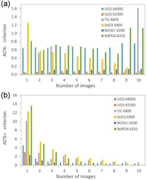
The data reported in Figure 5a indicate that the number of pixels removed (AC%- criterion) was independent of the number of images considered for image segmentation. Most of these pixels correspond to polishing defects (mainly scratches) and are analysed by the automatic segmentation procedure as grain boundaries, independent of the number of tilted images used for segmentation. This clearly indicates that the quality of the polishing is one of the main parameters that limits the efficiency of the automatic recognition of grain boundaries.
The number of pixels added to the segmented images (AC%+ criterion) decreased as a function of the number of images (n) used for the calculation of the segmented image. When this criterion is lower than approximately 0.5%, this corresponds to the addition of a few (typically 1–5) grain boundaries on the images that are not automatically detected (see Supplementary File S4). In this case, the number of missing grain boundaries is sufficiently low to not affect the calculation of the average grain size, and this
14 value for the AC%+ criterion can be an acceptable limit for the calculation of a high-quality segmented image. When considering the different materials studied, 6–10 images are generally suitable for achieving this AC%+ value, i.e. to automatically determine a high-quality segmented image without further manual correction. It appears that this range of values is independent of the magnification and the material studied.
Figure 5. Variation of the (a) AC%- and (b) AC%+ values (expressed in percentage) for segmented images obtained with n tilted images as a function of n. These parameters were measured for (U0.9Ce0.1)O2 at
15 Determination of the tilt angles
The choice of tilt angles can first appear as an important parameter for image segmentation processing. Thus, ten different sets of four out of the ten tilted images (previously recorded on a (U0.9Ce0.1)O2 ceramic) were used to extract the grain boundaries and determine the number of grains as
well as their average size. The average number of grains that was determined for every set of four images was 368 (± 8), while the number of grains determined from the complete dataset of ten images was 366 (Figure 6a). Thus, most of the grains present in the ROI were detected independently of the chosen tilt angles.
In parallel, the average grain diameter was measured from each set of four random images. The ten values are shown in Figure 6a. From these ten values, the mean value of the average grain diameters measured from the four-image random series was determined. It was equal to 2.34 (± 0.01) µm, while the average grain diameter determined for the entire ten tilted image series was 2.2 µm (Figure 6b). Thus, these values are very close, and the choice of tilt angles did not significantly modify the average grain diameter. The AC%+ and AC%- criteria values associated with each four-image random series are reported in Figure 6b as a function of the randomly selected images. Once again, the values of the accuracy criteria did not vary significantly according to the series considered.
These results indicate that the quality of the automatically segmented image does not depend on the tilt angles between the images. Thus, the tilt angles used to record the tilted image series can be chosen randomly between -5° and +5° without selecting specific tilt angles.
16 Figure 6. a) Average grain diameter and number of grains associated with the ten series of four images randomly selected within the dataset of ten images. b) AC%+ and AC%- values associated with the ten series of four images randomly selected within the dataset of ten images.
Recording 6–10 images with close but different tilt angles is a good compromise to obtain highly contrasted grain boundaries and to automatically and accurately determine a segmented image of the grains that are present in the ROI. The time required to record the SEM tilted image series was generally less than 15 min, while that required to compute the segmented image was less than 5 min.
Dependence on the user
The quality of image segmentation, which is often performed semi-manually or fully manually, can be user dependent. As some manual corrections can be performed using the SEraMic plugin by adding or deleting a few points, the average grain sizes determined from the same set of images by three different users are presented in Table 1 for comparison. The three sets of data were equivalent, and the result obtained, in terms of average grain size, was independent of the user.
17 Table 1. Compositions, sintering temperatures, and sintering times of the (U1-xCex)O2 ceramics. The
average grain diameters (D) and associated standard deviations (σD) that were determined in the present
study using the SEraMic method are also reported.
User 1 User 2 User 3
x T (°C) Time (h) Atm D (µm) σD (µm) D (µm) σD (µm) D (µm) σD (µm) 0.25 1300 10 Ar 2.06 1.05 2.15 0.95 1.98 1.10 0.25 1300 10 Ar-H2 0.14 0.08 0.15 0.07 0.17 0.09 0.14 1600 10 Ar-H2 7.01 4.05 7.30 3.48 7.76 3.73 0.10 1500 5 Ar-H2 1.51 0.71 1.58 0.55 1.49 0.68 0.10 1500 1 Ar-H2 0.75 0.27 0.68 0.29 0.67 0.34 0.10 1300 10 Ar-H2 0.18 0.08 0.14 0.07 0.20 0.08
Minimum grain size
Another important parameter is the minimum size of the average grain distribution that can be determined using the SEraMic method. To determine this, (U1-xCex)O2 ceramics with various average
grain sizes were studied. The average grain diameters (and associated standard deviations) are listed in Table 1, and the accuracy criteria associated with each ceramic were calculated. For the (U1-xCex)O2
ceramics containing the smallest grains (average grain size of approximately 150 nm), the images were recorded using magnifications higher than 20 k (corresponding to a 3.186 × 2.751 µm² image for 1024 × 884 pixels). Under these conditions, the vacuum quality in the SEM chamber was not sufficient to record more than six tilted images. Indeed, the sample surface was rapidly contaminated by the residual molecules present in the SEM chamber. Thus, the orientation contrasts were attenuated. This effect strongly limited the image quality, and thus the quality and reliability of the segmented image calculation.
The AC%+ (number of pixels added to the segmented images to complete the position of the grain boundaries) and AC%- criteria rapidly decreased when the average grain size increased (Figure 7). Considering that the SEraMic method allows the accurate and automatic determination of the grain boundary position when the AC%+ criteria is lower than 0.5, the lower limit of the grain size (diameter) that could be determined by the SEraMic method was close to 0.25 µm with the configuration of the
18 microscope used in this study. Apart from nanostructured materials, this allows the study of the majority of ceramic materials that are classically studied.
Figure 7. Variation in the AC%+ and AC%- values as a function of the average grain size for the (U1-xCex)O2
compounds. Corresponding averaged and segmented images are reported in Supplementary File S5.
Comparison of SEraMic with thermal etching
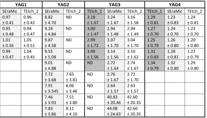
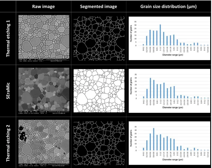
The robustness of the SEraMic method was tested by comparing the segmentation and average grain diameters determined using the SEraMic and thermal etching methods. To achieve this comparison, a series of transparent YAG ceramics was prepared by sintering at various temperatures and dwell times to monitor the average grain size. The image recording and segmentation processes were achieved after either thermal etching or recording of tilted image series on a mirror-like surface using the SEraMic method. The average grain sizes were determined automatically using the same procedure from the different segmented images (Table 2). On YAG3 and YAG4, thermal etching was performed first, and several zones of the samples were characterised (TEtch_1 in Table 2). The samples were then polished to obtain a mirror-like surface, and the same zones were characterised again using the SEraMic procedure (SEraMic in Table 2). Finally, all the samples were thermally etched, and the average grain size was characterised in the same zones (TEtch_2 in Table 2). A series of SEM images and related segmented images recorded on YAG4 are shown in Figure 8. The same grains were detected regardless of the
19 segmentation method considered (see Supplementary File S6). The grain sizes were determined from the grains observed in the segmented images. A total of 212 to 229 grains were observed in these images. The grain size distributions were very similar and independent of the segmentation method. The average grain sizes that were determined from each segmented image were 1.31 ± 0.83 µm (after the first thermal etching), 1.28 ± 0.81 µm (after sample polishing and use of the SEraMic method), and 1.27 ± 0.79 µm (after the second thermal etching). The variation in the average grain size remained limited and within the statistical tolerance interval, regardless of the segmentation method.
Table 2. Average grain diameters and associated standard deviations (expressed in µm) obtained from the YAG sample series of pellets determined from segmented images obtained using various techniques (TEtch = thermal etching). The average grain diameters determined from the same ROI by different methods are reported on the same line. Each line corresponds to analyses performed on different ROIs. (ND = not determined).
YAG1 YAG2 YAG3 YAG4
SEraMic TEtch_2 SEraMic TEtch_2 TEtch_1 SEraMic TEtch_2 TEtch_1 SEraMic TEtch_2 0.97 ± 0.41 0.96 ± 0.42 8.82 ± 4.70 ND 3.18 ± 1.67 ± 1.67 3.24 3.16 ± 1.58 1.29 ± 0.81 1.23 ± 0.83 1.24 ± 0.81 0.95 ± 0.48 0.94 ± 0.47 9.24 ± 4.84 ND 3.00 ± 1.47 2.94 ± 1.48 2.94 ± 1.49 1.27 ± 0.70 1.24 ± 0.70 1.23 ± 0.70 1.01 ± 0.56 1.05 ± 0.51 9.87 ± 4.58 ND 2.99 ± 1.72 ± 1.70 3.07 3.04 ± 1.70 1.25 ± 0.79 1.26 ± 0.80 1.20 ± 0.80 0.99 ± 0.47 1.04 ± 0.45 9.55 ± 5.08 ND 3.09 ± 1.56 ± 1.56 3.14 3.10 ± 1.62 1.31 ± 0.83 1.28 ± 0.81 1.27 ± 0.79 9.01 ± 4.88 ND ND 2.72 ± 1.64 2.74 ± 1.67 1.34 ± 0.79 1.32 ± 0.80 1.29 ± 0.80 7.72 ± 3.68 7.65 ± 3.81 ND 2.76 ± 1.67 2.72 ± 1.70 7.91 ± 3.545 8.06 ± 3.46 ND 2.64 ± 1.57 2.63 ± 1.57 7.46 ± 3.93 7.51 ± 3.80 ND 40.83 ± 20.46 42.60 ± 20.35 7.83 ± 3.86 8.11 ± 4.10 ND 44.08 ± 24.63 42.60 ± 20.35
20 Raw image Segmented image Grain size distribution (µm)
Th er m al e tc hi ng 1 SE ra M ic Th er m al e tc hi ng 2
Figure 8. Images recorded after the first thermal etching, after polishing for SEraMic analysis, and after the second thermal etching. All images were recorded on the same zone of the YAG4 sample.
Corresponding segmented images and grain size distributions are also reported (approximately 210–220 grains were considered in these images).
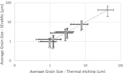
The average grain sizes determined using the SEraMic procedure are plotted as a function of the average grain size values obtained after thermal etching for comparison in Figure 9. There is a perfect match between the two datasets, indicating that the SEraMic method yields the same average grain values as the conventional method (image segmentation from images recorded on thermally etched materials). This is true for a large range of grain diameters (1–44 µm for the series of materials studied herein). Furthermore, the standard deviation around the mean grain size was identical, independent of the segmentation method. This is due to the fact that the same grains were recognised, and this indicates that the SEraMic method leads to a grain size dataset that is identical to the one provided by
21 classical methods. The SEraMic segmentation method is a robust method that combines reproducibility and reliability.
Figure 9. Comparison of the average grain sizes determined using a segmented image obtained with the SEraMic plugin on polished samples and after thermal etching on YAG samples. The same zones of the different samples were systematically studied.
In some cases, thermal etching can lead to precipitation or exudation of secondary phases. This phenomenon was observed locally in the YAG2 sample (Supplementary File S7). This can modify the sample microstructure and degrade the properties of the sample. Thus, thermal etching should be avoided with this type of material. In this case, the SEraMic method is particularly well adapted because no thermal treatment is required for image segmentation processing.
Conclusion
The SEraMic method, implemented in the SEraMic plugin for Fiji and ImageJ software, was developed to calculate a segmented image from a ceramic cross section that contains the information related to the grain boundaries. This method can be suitably used to determine the grain boundary positions of monophasic ceramics, metals, and alloys.
22 The SEraMic method is particularly well adapted for the characterisation of ceramic materials. It is fast, easy to implement, and provides very accurate segmented images showing grain boundaries and pores. The preparation of the cross section is one of the key factors for the fast calculation of an accurate segmented image because the sample surface must be polished to a mirror-like surface. The quality of the polishing should be perfect to eliminate all remaining scratches at the surface of the sample.
Recording the images only requires an SEM equipped with a BSE detector operating at a low acceleration voltage (3–10 kV), and a sample holder that can be tilted between -5° and +5°. Moreover, it is important to note that coating the sample is generally not required because the low-vacuum mode implemented in most conventional SEMs is suitable for recording BSE images on insulating materials. However, carbon coating remains a valid option because it does not modify the efficiency of the SEraMic method, but it does require a higher acceleration voltage (typically 8–10 kV).
With these few constraints, the SEraMic method provides an efficient way to accurately characterise the grain distribution of conductive and insulating materials with average grain diameters of as low as 250 nm. The acquisition time of the SEM tilted image series, which does not require any additional sample preparation after the polishing step, is low and typically ranges between 3 and 15 min for a series of six to ten images. The total time between the beginning of image recording and obtaining the final segmented image was less than 10 min. Moreover, the segmentation step is fully automated, with the possibility of modifying some parameters or correcting the automatically generated segmented image. Thus, all the grains present in the region of interest are detected automatically. In addition, because the procedure can be fully automated, it is important to underline that the segmented image does not depend on the choices of the operator.
The SEraMic method (and the SEraMic plugin) was implemented to study various types of ceramics (oxides, phosphates, and carbides) with results that are in good correlation with the grain sizes obtained using classical methods. It allows the researcher to save time by providing data related to the sample microstructure very quickly. The method can probably be extended to biphasic ceramics, but no trial has been performed during the development of the SEraMic method.
Acknowledgments: The authors would like to thank Yann Launay and Camille Perrière (IrCer, Limoges, France) for providing the YAG samples.
23 References
1 M.I. Mendelson, Average grain size in ceramics, J. Am. Ceram. Soc. 52 (1969) 443-446.
https://doi.org/10.1111/j.1151-2916.1969.tb11975.x
2 J.D. Katz, G. Hurley, Etching alumina with molten vanadium pentoxide, J. Am. Ceram. Soc. 73 (1990) 2151-2152.
https://doi.org/10.1111/j.1151-2916.1990.tb05292.x
3 U. Täffner, V. Carle, U. Schäfer, M.J. Hoffmann, (2004). Preparation and microstructural analysis of
high-performance ceramics, in: G.F. Vander Voort (Ed.), Metallography and Microstructures, Materials Park, OH: ASM International, 2004, pp. 1057-1066. https://doi.org/10.31399/asm.hb.v09.a0003795
4 I.O. Owate, R. Freer, Thermochemical etching method for ceramics, J. Am. Ceram Soc. 15 (1992) 1266-1268.
https://doi.org/10.1111/j.1151-2916.1992.tb05567.x
5 C. Garcı ́a de Andrés, F.G. Caballero, C. Capdevila, D. San Martı ́n, Revealing austenite grain boundaries by thermal
etching: advantages and disadvantages, Mater. Charact. 49 (2002) 121-127.
https://doi.org/10.1016/S1044-5803(03)00002-0
6 Y. Palizdar, D. San Martin, M. Ward, R.C. Cochrane, R. Brydson, A.J. Scott, Observation of thermally etched grain
boundaries with the FIB/TEM technique, Mater. Charact. 84 (2013) 28-33.
https://doi.org/10.1016/j.matchar.2013.07.003
7 T. Spusta, M. Jemelka, K. Maca, The comprehensive study of the thermal etching conditions for partially and fully
dense ceramic samples, Sci. Sinter., 51 (2019) 257-264. https://doi.org/10.2298/SOS1903257S
8 A.A. Felix, V.D.N. Bezzon, M.O. Orlandi, D. Vengust, M. Spreitzer, E. Longo, D. Suvorov, J.A. Varela, Role of oxygen
on the phase stability and microstructure evolution of CaCu3Ti4O12 ceramics, J. Eur. Ceram. Soc. 37 (2017) 129–136.
https://doi.org/10.1016/j.jeurceramsoc.2016.07.039
9 R. Heilbronner, Automatic grain boundary detection and grain size analysis using polarization micrographs or
orientation images, J. Struct. Geol. 22 (2000) 969-981. https://doi.org/10.1016/S0191-8141(00)00014-6
10 A. Coutinho, S.C.K. Rooney, E.J. Payton, Analysis of EBSD grain size measurements using microstructure
simulations and a customizable pattern matching library for grain perimeter estimation, Metall. Mater. Trans. A 48A (2017) 2375-2395. https://doi.org/10.1007/s11661-017-4031-z
11 H. Chen, Y. Yao, J. A. Warner, J. Qu, F. Yun, Z. Ye, S. P. Ringer, R. Zheng, Grain size quantification by optical
microscopy, electron backscatter diffraction, and magnetic force microscopy, Micron 101 (2017) 41–47.
http://dx.doi.org/10.1016/j.micron.2017.06.001
12 M. Ben Saada, X. Iltis, N. Gey, B. Beausir, A. Miard, P. Garcia, N. Maloufi, Influence of strain conditions on the
grain sub-structuration in crept uranium dioxide pellets, J. Nucl. Mater. 518 (2019) 265-273.
https://doi.org/10.1016/j.jnucmat.2019.02.052
13 R. Chinn, Grain sizes of ceramics by automated image analysis, J. Am. Ceram. Soc. 77 (1994) 589-592.
https://doi.org/10.1111/j.1151-2916.1994.tb07033.x
14 S. Wang, J. Waggoner, J. Simmons, Research summary graph-cut methods for grain boundary segmentation. JOM
63 (2011) 49-51. https://doi.org/10.1007/s11837-011-0111-5
15 A. Campbell, P. Murray, E. Yakushina, S. Marshall, W. Ion, New methods for automatic quantification of
microstructural features using digital image processing, Mater. Des. 141 (2018) 395-406.
https://doi.org/10.1016/j.matdes.2017.12.049
16 O. Dengiz, A.E. Smith, I. Nettleship, Grain boundary detection in microstructure images using computational
intelligence, Computers in Industry, 56 (2005) 854-866. https://doi.org/10.1016/j.compind.2005.05.012
17 M. Jungmann, H. Pape, P. Wißkirchen, C. Clauser, T. Berlage, Segmentation of thin section images for grain size
analysis using region competition and edge-weighted region merging, Computers & Geosciences, 72 (2014) 33-48.
https://doi.org/10.1016/j.cageo.2014.07.002
18 M. Li, D. Chen, S. Liu, F. Liu, 2020. Grain boundary detection and second phase segmentation based on multi-task
learning and generative adversarial network, Measurement 162, 107857.
https://doi.org/10.1016/j.measurement.2020.107857
19 G.F. Vander Voort, Grain size measurement methods: A review and comparison, Microsc. Microanal. 19 (2013)
1760-1761. https://doi:10.1017/S1431927613010799
24 20 H. Abrams, Grain size measurements by the intercept method, Metallography, 4 (1971) 59-78.
https://doi.org/10.1016/0026-0800(71)90005-X
21 H. Abrams, Practical applications of quantitative metallography," in Stereology and Quantitative Metallography,
ed. G. Pellissier and S. Purdy (West Conshohocken, PA: ASTM International, 1972), 138-182.
https://doi.org/10.1520/STP36848S
22 G.F. Vander Voort, Committee E-4 and Grain Size Measurements: 75 Years of Progress, Standardization News 19,
(1991) 42-47. https://www.metallography.com/grain.htm
23 C.A. Schneider, W.S. Rasband, K.W. Eliceiri, NIH Image to ImageJ: 25 years of image analysis, Nat. Methods 9
(2012) 671-675. https://doi.org/10.1038/nmeth.2089
24 J. Schindelin, I. Arganda-Carreras, E. Frise, V. Kaynig, M. Longair, T. Pietzsch, S. Preibisch, C. Rueden, S. Saalfeld, B.
Schmid, J.-Y. Tinevez, D.J. White, V. Hartenstein, Kevin Eliceiri, P. Tomancak, A. Cardona, Fiji: an open-source platform for biological-image analysis, Nat. Methods 9 (2012) 676-682. https://doi.org/10.1038/nmeth.2019
25 A. Maître, D. Beyssen, R. Podor, Modelling of the grain growth and the densification of SnO2-based ceramics,
Ceram. Int. 34 (2008) 27-35. https://doi.org/10.1016/j.ceramint.2006.07.008
26 D. Qin, A. Mesbah, J. Lautru, S. Szenknect, N. Dacheux, N. Clavier, Reaction sintering of rhabdophane into
monazite-cheralite Nd1-2xThxCaxPO4 (x = 0 – 0.1) ceramics, J. Eur. Ceram. Soc. 40 (2020) 911-922.
https://doi.org/10.1016/j.jeurceramsoc.2019.10.050
27 H. Aréna, M. Coulibaly, A. Soum-Glaude, A. Jonchère, A. Mesbah, G. Arrachart, N. Pradeilles, M. Vandenhende, A.
Maitre, X. Deschanels, SiC-TiC nanocomposite for bulk solar absorbers applications: Effect of density and surface roughness on the optical properties, Sol. Energy Mater. Sol. Cells 191 (2019) 199-208.
https://doi.org/10.1016/j.solmat.2018.11.018
28 T. Perez, L. Latu-Romain, R. Podor, J. Lautru, Y. Parsa, S. Mathieu, M. Vilasi, Y. Wouters, In situ oxide growth
characterization of Mn-containing Ni–25Cr (wt%) model alloys at 1050°C, Oxid. Met. 89 (2018) 781–795.
https://doi.org/10.1007/s11085-017-9819-0
29 Application Note: Information from Every Angle. Directional BSE Detector for Next-Level Imaging,
http://emc.missouri.edu/wp-content/uploads/2016/03/FEI-Information-for-Every-Angle-DBS-Detector.pdf
30 D. B. Ballard, A procedure for calibrating the magnification of a scanning electron microscope using NBS SRM 484,
NBSIR 77-1248, U.S. Department of Commerce, National Bureau of Standards, June 1977.
https://nvlpubs.nist.gov/nistpubs/Legacy/IR/nbsir77-1248.pdf
31C. Lafond, T. Douillard, S. Cazottes, P. Steyer, C. Langlois, Electron CHanneling ORientation Determination
(eCHORD): An original approach to crystalline orientation mapping. Ultramicroscopy 186 (2018) 146-149.
https://doi.org/10.1016/j.ultramic.2017.12.019
32 D. Gruner, Z. Shen, Direct scanning electron microscopy imaging of ferroelectric domains after ion milling, J. Am.
Ceram. Soc. 93 (2010) 48–50. https://doi.org/10.1111/j.1551-2916.2009.03392.x
33 R. Wuhrer, K. Moran, Low voltage imaging and X-ray microanalysis in the SEM: challenges and opportunities, IOP
Conf. Ser.: Mater. Sci. Eng. 109 (2016) 012019. https://doi.org/10.1088/1757-899X/109/1/012019
34 D.J. Stokes, Principles and practice of variable pressure/environmental scanning electron microscopy (VP-ESEM).
2008 John Wiley & Sons, Ltd. 221 pages. https://doi.org/10.1002/9780470758731
35 D. Lowe, Distinctive Image Features from Scale-Invariant Keypoints. Int. J. Comput. Vis. 60 (2004) 91-110.