A general approach for the microrheology of cancer cells by atomic force microscopy

HAL Id: hal-00759704

https://hal.archives-ouvertes.fr/hal-00759704

HAL is a multi-disciplinary open access archive for the deposit and dissemination of sci-entific research documents, whether they are pub-lished or not. The documents may come from teaching and research institutions in France or abroad, or from public or private research centers.

L’archive ouverte pluridisciplinaire HAL, est destinée au dépôt et à la diffusion de documents scientifiques de niveau recherche, publiés ou non, émanant des établissements d’enseignement et de recherche français ou étrangers, des laboratoires publics ou privés.

A general approach for the microrheology of cancer cells

by atomic force microscopy

Biran Wang, Pascal Lançon, Céline Bienvenu, Pierre Vierlingb, Christophe Di

Giorgio, Georges Bossis

To cite this version:

Biran Wang, Pascal Lançon, Céline Bienvenu, Pierre Vierlingb, Christophe Di Giorgio, et al.. A general approach for the microrheology of cancer cells by atomic force microscopy. Micron, Elsevier, 2013, 44, pp.287-297. �10.1016/j.micron.2012.07.006�. �hal-00759704�

A general approach for the microrheology of cancer cells by

Atomic Force Microscopy

Biran Wang,

Pascal Lançon,

Céline Bienvenu,

Pierre Vierling,

Christophe

Di Giorgio

and Georges Bossis

†

Laboratoire de Physique de la Matière Condensée (LPMC), CNRS UMR 7336, Université de Nice-Sophia Antipolis, Parc Valrose 06108 Nice cedex France 2;

‡_{Institut de Chimie Nice, UMR 7272, Université de Nice Sophia Antipolis, CNRS, 28, Avenue de}

Valrose, F-06100 Nice, France.

Abstract

The determination of the viscoelastic properties of cells by atomic force microscopy (AFM) is mainly realized by looking at the relaxation of the force when a constant position of the AFM head is maintained or at the evolution of the indentation when a constant force is maintained. In both cases the analysis rests on the hypothesis that the motion of the probe before the relaxation step is realized in a time which is much smaller than the characteristic relaxation time of the material. In this paper we carry out a more general analysis of the probe motion which contains both the indentation and relaxation steps, allowing a better determination of the rheological parameters. This analysis contains a correction of the Hertz model for large indentation and also the correction due to the finite thickness of the biological material; it can be applied to determine the parameters representing any kind of linear viscoelastic model. This approach is then used to model the rheological behavior of one kind of cancer cell called Hep-G2. For this kind of cell, a power law model does not well describe the low and high frequency modulus contrary to a generalized Maxwell model.

Keywords: Microrheology, Cancer cell, Atomic force microscopy, Biomechanics and Viscoelasticity.

*

Correspondence author: Georges Bossis Tel: +33 492 076 538

Fax: +33 492 076 536

1 Introduction

The rheological properties of single cells have been investigated in the past using a large variety of methods like micropipette aspiration[1], traction or compression between two microplates[2], optical tweezers[3,4], magnetic twisting cytometry[5,6], rotational microrheology[7], atomic force microscopy (AFM)[8–10] and many other methods. All these methods (except micropipette aspiration) have in common the tracking of a micro or a nanoparticle either at the surface of the cell or even inside the cell in response to an applied force. Then a model is needed to relate the force-displacement curve to the viscoelastic properties of the cell. If the probe is larger than the characteristic mesh size, , of the actin network (typically =100nm) a continuum approach can be used to model this response. A possible approach rests on a two fluid description with a viscoelastic network coupled by a frictional force to a viscous fluid [11]. The approximation of low Reynolds number can be written as:   2 Re   1   al  G (1)

with a the radius of the probe, l the amplitude of motion of the probe and  the density of the fluid. The order of magnitude of a and l being the micron and the order of magnitude of G() being between 0.1 and 10kPa it is readily seen that this condition holds even for frequencies as high as 100kHz. The other condition needed for the use of a frequency generalized Stokes’ law is that a compressive wave in the elastic network would be overdamped on a characteristic length equal to the dimension of the probe; this is realized for frequencies above[11,12]:   2 2      b a (2)

where  and  are Lamé coefficients and ~/2 is the friction coefficient between the fluid phase and the elastic network. Introducing  with G the static shear modulus, the crossover frequency becomes:

2 1          _{  } b a (3)

We shall see in the following that the order of magnitude of the relaxation time is the second , so we get b~10-2; it means that the deviation from generalized Stokes’ Einstein equation is

only expected at very low frequencies, that is to say on a long time scale. In AFM experiments, as well as with optical tweezers the bead is not completely immersed in the viscoelastic medium, so this continuum approach must be modified to take into account different boundary conditions. When the motion of the probe is perpendicular to the surface as in AFM or indentation experiments, the basic relation which can be generalized in the frequency or time domain is no longer the Stokes law , but the Hertz law which applies to a spherical probe which settles in an elastic medium Due to the change of the contact surface with time, the time dependent generalization of the Hertz law, which rests on the hypothesis of a linear superposition of delayed response to increments of force or displacement, must be properly written. Such a generalization was described, for instance in Johnson [13] and applied to nanoindentation of cells [14]. As the cell thickness is often not very large compared to the indentation depth, a correction of the Hertz formula has been proposed [15] for elastic media which introduces a function of the indentation depth over the cell thickness.

This correction was used to model the time dependent response to an approximate step displacement, with the approximation that during the relaxation of the force, the indentation depth could be considered as constant [16]. Besides the time dependent generalization of the Hertz model including the cell thickness correction, a description of the viscoelastic response function of the material is needed. In principle a deconvolution should allow to extract the creep response function G(t) or the compliance function J(t) but, due the limited range of time -or frequency- in the experiment, it is more direct to fit the experimental curve with a model response function. Furthermore the viscoelastic models can give some insight in the physical process underlying their representation. One of the most common models to describe a viscoelastic solid is the Zener model consisting of a Maxwell element in parallel with a spring representing the zero frequency elastic modulus G0, the Maxwell element introduces a

relaxation time:    i i i G (4)

This simple model of viscoelastic solid containing three parameters, can describe quite well the mechanical response of different kinds of cells[17,18], nevertheless some other experiments show a more complex response which can be described by a set of relaxation times or by a power law. In this last case an interpretation of the power law behavior was proposed in terms of a distribution of relaxation times associated with a power law for the distribution of the lengths of the elementary units of the actin network which was supposed to present a fractal structure[19]. The mechanical response of a cell to different stimuli is important, because several biological functions are regulated by their contact with the neighboring cells or the extracellular matrix [20]. On the other hand it has recently been demonstrated that a small mechanical stimulus induced by the periodic motion of magnetic nanoparticles at the surface of the membrane can cause the death of the cell[21,22]. Since a magnetic field can easily be applied in vivo it could be an attractive way to destroy tumors if the magnetic nanoparticles specifically bind to the cancer cells. In this paper our objective is to obtain the rheological characterization of a given type of cancer cells in order to use it in a future work to model the motion of different kinds of magnetic nanoparticles deposited on the surface of the cells. The knowledge of the viscoelastic response of the cell to the AFM probe will allow to determine the deepness at which magnetic particles can penetrate when submitted to an oscillating magnetic field of different frequencies. An atomic force microscope was used and in a first section we describe briefly the operating conditions and the biological material. As explained above, different approximated methods are used to identify the viscoelastic parameters from the experiments, so the second section will be devoted to a presentation of the equation used to deduce the material properties from the indentation depth versus time of a spherical indenter, and the prediction of this equation will be tested against the trajectory of the bead deduced from a finite element simulation which mimics the operating condition of the AFM. In the third section the results are analyzed through different rheological models and it is shown that the generalized Maxwell model gives a better agreement with the experimental data than a power law model.

2 Materials and methods

Besides imaging, another major application of AFM is force spectroscopy through the direct measurement of tip-sample interaction forces as a function of the indentation depth of the tip into the sample. Compared to conventional rheometers the use of AFM to get rheological properties raises three problems. The first one is the determination of the position of the

probe relatively to the surface, the second one is due to the fact that the contact surface between the probe and the biological material is changing during the experiment and at least we have no independent measurement of the position of the probe and of the applied force. As presented in the introduction there are many papers dealing with these problems and we do not intend to make a review of them here, but just to present what we think to be the best way to overcome them.

2.1 Cancer cells

The tumor cell which has been studied is called Hep G2, a human liver carcinoma cell line. HEP-G2 cells were grown at a BD Falcon™ 35mm Easy-Grip™ Cell Culture Dish, in Dulbelcco modified Eagle culture medium (Invitrogen, Carlsbad, CA) containing 10% fetal calf serum, glucose (4.5g/L), glutamine (2mM), penicillin (100units/mL), 10 mg/mL gentamycin in a wet (37°C) and 5% CO2/95% air atmosphere.

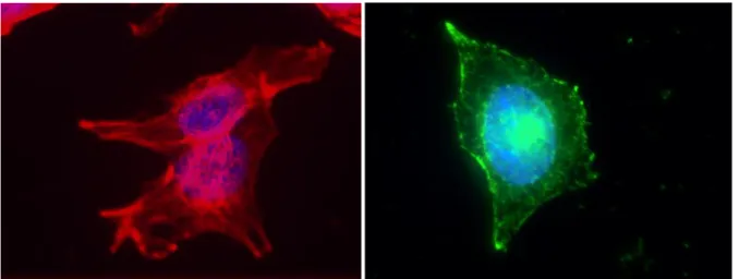
Fig. 1: The organization of actin (left) and microtubules (right) of Hep G2 shown by fluorescent microscopy

For fluorescence microscopy, HepG2 cells were grown on glass cover slips for 48h and fixed with 4% paraformaldehyde for 15 min. Cells were then permeabilized with PBS 0,1% triton. For microtubule staining, cells were incubated with anti beta-tubulin followed by secondary anti mouse antibody coupled to Alexa-488 (Molecular Probe). For actin staining, cells were incubated with phalloidin (Sigma Aldrich). Nuclei were stained with Hoescht. Cover slips were mounted on slides using Permafluor (Thermo Scientific) and observed with Zeiss Axioimager microscope.

The organization of actin and microtubules are shown separately, respectively on the left and right hand side of Fig.1. The nucleus is stained in blue. It appears that the microtubule network is homogeneous and dense right above the nucleus.

2.2 Force spectroscopy with AFM

Atomic force microscopic experiments were performed with an Agilent series 5100 AFM/STM (Agilent, Santa Clara, CA). The probe of AFM which have been used to obtain the rheology of cancer cells is a spherical borosilicate glass probe (Novascan, Ames, IA). The spring constant of the cantilever is obtained by using an AFM option called Thermal K. which calculates the cantilever spring constant through the use of the equipartition theorem who states that the kinetic energy stored in a system, here on a coordinate which is the

deflection of a cantilever from its equilibrium position, is equal to one half of the thermal energy of the system[23]. The spring constant of spherical borosilicate glass probe was 0.047N/m. The radius of the spherical probe was: R= 2.5 m.

The deflection d, of the cantilever is related to the applied force by:

 

   

F t kd k z t h t (5)

Where z(t) is the position of the piezoelectric transducer and h(t) the indentation depth. This equation only applies when the indentation begins that is to say for a given position z0(t). For

positions above the surface, the deflection can change a little bit for the highest velocity of the cantilever due to the viscosity of the feeding liquid; the corresponding force is subtracted as indicated below. In a "force spectroscopy" mode a first detection of the surface is related to a given indentation force which is taken as a (false) reference surface by the AFM, which needs to be corrected. A fit of the indentation curve with two parameters (the surface position and the shear modulus) is the more usual procedure. Another technique consists in comparing the work done during different indentations which are stopped at a same given trigger force. The work done is the integral of the force displacement curve whose value is quite insensitive to the position of the surface, so, supposing the validity of the Hertz formula, it allows to relate the ratio of the shear modulus at different positions of the cell to the ratio of the indentation depths[24]. This is very convenient for cartography of the shear modulus of the surface of a cell, nevertheless a reference point is needed and, above all, this method relies on the validity of the Hertz equation.

We propose here a different method which allows to determine accurately the contact point of the probe with the surface and the time dependence of the force. The process is exemplified in Fig. 2 where, the upper plot is the applied force versus time, and the lower one is the displacement of the piezoelectric head versus time. The (false) surface is found by setting an arbitrary force for which the piezo will stop and set z=0; this is the initial point at t=0 in Fig. 2 (sketch A), then the piezo retracts during 10s at a given velocity and stops 2µm above this initial position (sketch B) and remains in this position during 10s to reach a plateau (P) on the force curve. Since this plateau in the feeding liquid corresponds to a zero force we use it to find the time tsf and the corresponding position zsf of the piezo where the bead leaves the

surface. It only needs to extrapolate the horizontal plateau when the probe is at rest well above the surface (t=15~20s in Fig. 2), to get the time t1 where the bead leaves the surface and then the corresponding position (point 2) zsf of the piezo head which is associated with

the surface of the cell: h=0. After that, the cantilever head is lowered at a given velocity (from 100µm/s to 100nm/s), depending on our experiment need, and stopped at a given position(sketch C) which is kept constant during 50s; during this time the probe continues to deep and the force is relaxing(sketch D). Note that the time t2 where the bead leaves the

surface was obtained from the previously determined position of the surface zsf (point 3 left

insert) and so the force, F2, corresponding to this time t2 (point 4 on the insert) can be

precisely determined Finally, the piezoelectric head is raised in 10s towards its initial position at time t=0; and in all our measurements we recovered the same force as the initial one (red dashed curve), showing that we did not enter into the plastic regime. Finally this procedure also gives us access to the hydrodynamic force on the cantilever: F(t2)-F(t1) which should be subtracted from the total force [25]. Even for high velocities, here 3µm in 0.01s, this hydrodynamic force is rather small (around 2nN) compared to the total force and, of course, does not play a role on the relaxation part of the force.

Fig. 2: Left is an indentation cycle; right is the method for the determination of the contact point and of the force/indentation curve. Upper graph: experimental force

versus time. Lower graph: motion of the cantilever head versus time

The last important thing to note in this Fig. 2 is the fact that when the piezo returns to its initial position (red dash line on both graphs) the initial force is also recovered. It is a proof that there is no plastic deformation of the medium and the recovery time is about 10s in this example.

2.3 Microrheology with a spherical indenter 2.3.1 Time dependent Hertz model

The quasi-static force is related to the indentation depth by the Hertz equation [26,27]:

3 2 2 4 3 1    E F R h (6)

where E is the Young modulus and R the radius of the spherical probe. In the absence of information on the Poisson ratio, it is usual to consider the cell as an incompressible medium and to take =0.5 and E=3G where G is the shear modulus; in this case:

3

2 16

3

  R

It is interesting to note that the Hertz formula can be recovered, within a constant number, by considering that the average strain, , for an indentation depth, h, is given by:

1 2

2 2

  h h  h

a Rh R (8)

with a the radius of the contact area. The average force is then:

1/ 2 3/ 2

2 2

   

  

F G S G Rh G R h (9)

The dependence in R1/2 h3/2 predicted by the Hertz law is recovered under the approximation <<1. We shall see in the following that, in our experimental conditions, the Hertz formula needs to be corrected. In normal or cancer cells, more than 98% of molecules are water [28], and their viscoelastic properties result from the interaction between water and a poroelastic medium formed by the actin skeleton of the cell. A quite general description of a viscoelastic solid is given by the generalized Maxwell model consisting in a purely elastic part of shear modulus G0 in parallel with a series of Maxwell units, representing different relaxation

processes modeled by a set of relaxation times[15,26,27].

In the frame of the linear theory of viscoelasticity the increment of stress at a time t resulting from a stepwise increment of strain at time t' is given by:

   '  '

   

d t G t t d t (10)

Where G(t) depends on the viscoelastic model under consideration. For instance, for the generalized Maxwell model, we have:

 

It is important to note that the Eq. 10 is not directly relevant to the case where the contact surface between the medium and the tool is changing with time, which is presently the case. Actually the time dependent generalization of the Hertz model starts with Eq. 7. The increment of force at time t is related to the increment of indentation at time t': dh(t') by:

 



  

' '

 

dF t CG t t dh t (12)

Integrating the Eq.12 gives:

     3 2 0 ' ' ' ' 

_



This is a general formula for a spherical probe indenter, the rheological properties of the material being represented by the stress response function: G(t). The same kind of reasoning with the compliance response function J(t) will give:

          3 2 0 ' 0 ' ' '  _   _ 



with C'=1/C

The relation between the two response functions is obtained by taking the Laplace transform of the respective convolution products, which will give:

   _ 2

G p J p p (16)

Eqs. 14 and 15 are simply time dependent generalizations of the Hertz formula. If the relative indentation depth h/R, or the indentation depth relatively to the thickness of the sample: h/L, are not much smaller than unity, then these formula need to be corrected, that is what we are going to see in the next section.

2.3.2 Corrections to the Hertz model

The Hertz model is known to be accurate only for small values of the contact area with respect to the radius of the probe. For larger indentation the corrections depend on the Poisson ratio [29,30]. In order to find a correction adapted to our experimental conditions, we took =0.5 and compared, for a large indentation, the force calculated by FEM with the Hertz equation for a purely elastic cylindrical plate whose thickness and radius were very large compared to the probe radius (R=2.5m). The thickness L and the radius of the cylinder were both taken equal to 200µm. The Young modulus E was 575Pa corresponding to a value measured on a cancer cell. We found a small difference (4% for h=1m) between the Hertz equation and the result obtained by FEM. Introducing a first order correction factor in the Hertz equation (Eq.17), gave a result which very well reproduces the FEM result until h/R=0.4 :





On the other hand the Hertz equation was corrected for the effect of the finite thickness, L, of the sample by (14):





Once again, there is a small difference between this modified Hertz equation Eq.18 and FEM result, but this difference disappears if we use the same correction as in Eq.17 Finally the corrected expression of the Hertz model, Eq.20, is found to be in excellent agreement with the FEM result at least for indentation below 20% of the plate thickness.





The time dependent generalization Eq.20 is straightforward. Let us call g(h) the function which multiplies the Hertz equation:

  1   10    _{ }   h g h f h R (21)

Then, instead of applying the time superposition to h3/2 it should be applied to h3/2 g(h) so Eq.13 becomes:    





_











Before applying Eq. 23 to find the function G(t) from an experiment it is worth testing its application to a viscoelastic solid represented by the popular Zener model.

2.3.3 Derivation of the probe trajectory in a viscoelastic medium

We wish to predict the trajectory of the spherical probe inside a viscoelastic solid represented by the Zener model consisting of a spring of modulus G0, in parallel with a Maxwell element

represented by a spring G1 and a dashpot of viscosity 1. For this model the response function

to a unit stress step is:

  1 0 1     t z G t G G e (24)

where 1=1/G1 is the relaxation time of the Maxwell branch. Then from Eq.23

     3/ 2









_

Deriving Eq. 25 and taking into account that:

  1  1  3/ 2





and (cf. Eq.5) that:F t

 

   

    _{ }         3/ 2 0 1 1 1 3/ 2 0 1 1 10 3 1 1 10 10 2 10   _{ }       _ _           _{ }  _  _  _{ }       τ τ τ dz h z h h G h C h f h dt R dh dt h h h G G Q h f h h f h R R R (27) where   0 02 3/ 2 3 2 3/ 2 2 0 3 2 2 52 0 0 0 0 2 2 3 3 4 4 4 12 4 32 3 15 5   _  _  _  _             _  _  _  _     R R R R Q h h h h h L L L L (28)

In order to check the validity of this approach the indentation and the force versus time are calculated from Eq. 27 and compared with the result obtained from a simulation done with the software Abaqus which contains the possibility to introduce the viscoelastic parameters of the Zener model. A 2d axisymmetric geometry was used; the cantilever was represented by a spring of stiffness 0.05N/m and the spherical probe by a rigid sphere (Fig. 3). The cell was modeled by a cylinder of thickness L whose viscoelastic properties, defined by the Zener model, were the following: G0=191.6Pa, G1=118.4Pa, 1=8.4s which are values obtained for

a given cancer cell.

Fig. 3: Calculation of the force with respect to the indentation in a viscoelastic medium with a spherical probe mounted on a spring using the software Abaqus

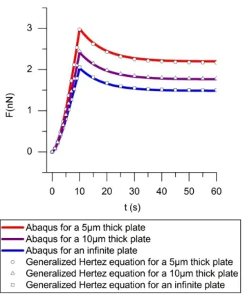
The result is shown in Fig. 4 where the force was plotted versus time when a displacement at a velocity of 0.1m/s during 10 seconds was applied to the top of the spring and then stopped at z=1µm. The numerical solution of the differential equation Eq.27 was compared to the Abaqus result for a cylinder whose thickness is infinite (in practice L=200µm in Abaqus) and for finite thicknesses of 5 and 10µm. Fig. 4 shows a very good agreement between FEM calculation and the solution of Eq.27 in all the cases, so we can trust the validity of the corrections applied to the Hertz formula and its generalization to time dependent forces. It is also worth noting that it applies for any function z(t) and in particular for a sinusoidal one.

Fig. 4: Comparison between FEM result and the solution of Eq. 27 for the indentation versus time in disk of different thicknesses.

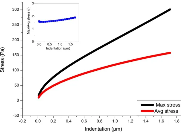
Another interesting point revealed by the FEM calculation is that the maximum stress generated by the motion of the spherical probe is not situated directly on the surface of the probe but below, on the axis of indentation (cf. Fig. 3) This maximum stress depends on the indentation depth and, as long as no plastic flow is experimentally observed, it determines the range of stress that the cell can support without yielding. In Fig. 5 is plotted, in the case of a purely elastic medium, the evolution of the maximum stress with the indentation depth. The average stress can be approximated by putting: =F/(2Rh) with F given by Eq.20. Of course this average stress is lower than the maximum stress (cf. Fig. 5), but it is quite remarkable that the ratio between the maximum stress and the average one, remains approximately constant with the indentation at a value of about 1.6 up to 0.6m and then increases slowly until 1.8 for a deepness of 1.7µm.

Fig. 5 : Maximum and average stress with respect to the indentation depth for a purely elastic medium; the diameter of the bead is 5µm and the thickness of the layer is 10µm;

the insert is the ratio of maximum stress to average stress 2.3.4 Deriving the material properties

Eq.25 is a general equation relating the force, F(t), and the indentation, h(t), which are both known experimentally, to the response function G(t). In principle it is possible to extract G(t) by taking the Laplace transform of the convolution product in order to get G(p) and then to come back by inverse Laplace transform to G(t). Nevertheless ,the time scale on which the force is measured is not infinite as in a convolution product and the experimental data can be noisy, so the error coming from this double Laplace transform is difficult to evaluate; furthermore , even if we can get a reliable result for G(t), we would like to compare it with known models. In practice it is much easier to directly begin with a given model for G(t)-like for instance the generalized Maxwell model- and to see afterwards if this model can well represent the experimental curve. As an example of this procedure let us suppose that the function G(t) of Eq. 11 well describes the viscoelastic properties of the material; then inserting it in Eq.23 gives:

   3/ 2     0 1 ( )      _  _ 







In a fit of the parameters G0, Gi, i, (i=1, n), the force F(t) is the experimental function whose

values are known for a given set of time values: Fexp(tj) (j=1,N) and the left-hand side of

Eq.(29) is the "theoretical" part: Fth(tj,G0,Gi,i) containing the unknown parameters. The

minimization of the residue, using the Levenberg-Marquardt method allows to find the unknown parameters. This procedure can, of course, be used for any kind of function G(t) and will be used in the following both for the generalized Maxwell model (Eq.11) and a power law relaxation function: G(t)=At

3 Results

As explained in section 2.2 all the experimental curves have been obtained in force spectroscopy mode with different velocities of the piezoelectric transducer on which is attached the cantilever head. The final position was corresponding to an indentation depth of about 1m. The small viscous force coming from the hydrodynamic friction of the cantilever in the feeding liquid was subtracted and the indentation depth, h(t), was obtained as shown in Fig. 2. The indentation was stopped at a time t=ts. If there was no relaxation during the rising

time, or in other words if ts<<i, then the terms Fi(t) in Eq.29 are negligible and the force at

t=ts can be expressed as:

   3/ 2



 





This is the hypothesis which is usually done [17][18] when dealing with the relaxation part for t>>ts. It means that at t=ts, which is the starting point of the relaxation curve, Eq.30 gives

access to the sum of the shear moduli of the model, which is called the high frequency modulus:

0 1 2

   

G G G G (31)

On the contrary, if the time ts is longer than all the relaxation times, the integrand

representing Fi(t) in Eq.29 will be different from zero only for t-t'< where ts, so the term

containing h(t) can be taken out of the integral in Fi(t) with its final value h(ts); then

considering that ts>>i we shall end up with:

   3/ 2





0



s s s

F t CG h t g h t (32)

This is now the low frequency limit of the shear modulus which is measured at t=ts but in this

situation the indentation is a quasi static one and after stopping there will be no relaxation. This is the way to obtain the static shear modulus G0.

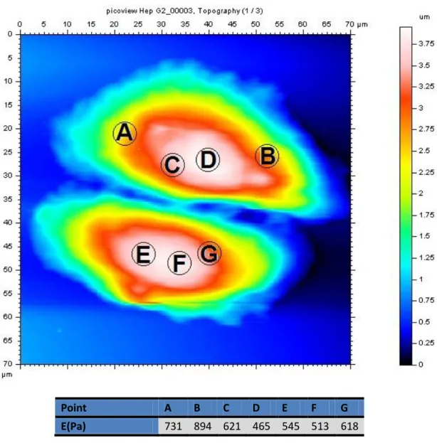
Point A B C D E F G E(Pa) 731 894 621 465 545 513 618

Fig. 6: AFM topography of Hep G2 cell, the point A to G are the measurements where has been carried out

All the experiments that we are going to discuss were made on the central part of the cell where the height of the cell is maximum and is about 4 m. Actually, as shown in Fig. and in the table just below, the values of G0 do not vary significantly for different points in the

region above the nuclei in the white zone (points E, F, D), but they increase when the measurement is done closer to the border of the cell. These measurements were made in a quasi static way; on the other hand, if only the relaxation part of the force is used then ts

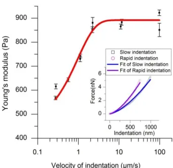
needs to be as small as possible to minimize the error, but in any event it will be safer to fit the full curve from the beginning of the indentation. In order to illustrate this point we have presented in Fig. 7 the values of the shear modulus which are obtained from Eqs. (30) or (31) after an indentation made at different velocities on the same cell. It clearly shows that the shear modulus obtained in this way depends on the indentation velocity but this value has no clear meaning in the frame of the viscoelastic models and only a fit of the total indentation curve can allow to attribute safely the values of the fitted parameters to a given model as we shall see in the next section.

Fig. 7: Young’s modulus versus indentation velocity. In the insert: force versus indentation for two different velocities (v=100µm/s and 100nm/s) and their fit by Eq. 20 3.1 Response function G(t) of the cells Hep G2

A typical curve representing the force versus time for a "slow" velocity of the cantilever: v=0.25µm/s is plotted in Fig. 8; the indentation depth corresponding to the maximum of the force is hs=1.08µm. The force (black square line) passes through a maximum when the

cantilever stops and then decreases as the probe continue to go down until the elastic stress becomes equal to the stress applied by the cantilever. This curve was fitted with the generalized Maxwell model with a single branch (Zener model) for the 3 parameters: G0, G1, 1.

Fig. 8: Applied force versus time during an indentation with a velocity: v=0.25µm/s and a maximum indentation depth: hs=1.08µm .The blue triangles represent a fit with a

power law for G(t) and the red circles a fit with a one branch Maxwell model As can be seen in Fig. 8, the fit is good on all the time scale for the following parameters: G0=198Pa, G1=101Pa, 1=7.1s. This model was also observed to give a good representation

of the viscoelasticity of some bacterial cells[18] and of chondrocytes[17]. Nevertheless it is worth noting that in these previous works the fit was only done on the relaxation part of the curve, supposing that the indentation was fast enough so that the medium did not have time to relax during the indentation. If this hypothesis was used for the experiment represented in Fig. 8 the relaxation part would be fitted by the function:

  3/ 2   1 0 1 when        _  _    s t t s s s s F t t Ch g h G G e t t (33)

where ts and hs are respectively the time and the indentation corresponding to the maximum

of the force. In our example it would give G0=203Pa, G1=70Pa, 1=8.4s instead of

G0=198Pa, G1=101Pa, 1=7.14s. The error is not that big, the maximum error being 40% for

G1, nevertheless the degree of approximation of Eq.33 depends on the importance of G1

compared to G0 and on the relaxation time 1 compared to ts since it supposes that for t=ts the

modulus is equal to G0+G1, that is to say that the material did not have time to relax during

the rising indentation.. On the other hand it is clear that the velocity of the cantilever head will give a limit on the smaller relaxation time which can be detected: roughly speaking a relaxation time which would be smaller than ts would not be detected. In practice our Hep G2

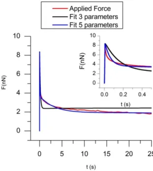
cell gives a good example of this remark. In Fig. 9 is plotted the force versus indentation for a velocity of the piezoelectric head: v=250µm/s and about the same indentation depth hs=1.27µm. The maximum of the force is higher than in Fig. 8, and above all, shows a very

fast relaxation of large amplitude. A fit of this curve with a single relaxation time, 1, (red

circle curve in Fig. 9) no longer works, and it is necessary to add another relaxation time, 2,

to give a satisfying agreement (blue triangle curve).

velocity: v=250µm/s. Red dots represent a fit with 3 parameters (the Zener model) for G(t) and the blue triangles a fit with 5 parameters (two Maxwell branches)

The results obtained on several experiments both for fast and slow indentation velocities are summarized in Tab 1. In parentheses are the values calculated without taking into account the thickness of the cell which overestimates the moduli of about 15-20% because the increase of stiffness due to the presence of the bottom wall was attributed to the elasticity of the cell. The rapid relaxation time 2=0.06s associated with a modulus G2 of about 450Pa means that some

elastic part of the cytoplasm, whose elasticity is more than two times larger than the static one, is associated with a rather low friction during its relaxation (2=2G2=27Pa.s) compared

to the one associated with the slow relaxation process (1 =1G1=450Pa.s). In previous

experiments, either with AFM [18] or with specific devices like microplates [2], the time scale of the indentation or of compression in the case of microplates was much longer so a Zener model with a single Maxwell time as in Fig.8 was able to represent the viscoelastic behavior of the cell and this fast relaxation time associated with a lower viscosity was not detected. Slow indentation G0 G1 1 Average 210 (247.6) 118.4 (128.3) 5.6 (6.1) Standard deviation 22.8 (28.5) 19.8 (20.7) 2.1 (2.2) Rapid indentation G0 G1 1 G2 2 Average 184.3 (214.5) 149.4 (168.6) 3.07 (3.84) 451.4 (538.5) 0.057 (0.065) Standard deviation 65.8 (74.0) 30.2 (35.1) 0.99 (1.16) 110.2 (142.7) 0.003 (0.018)

Tab 1: Viscoelastic parameters deduced from a fit of G(t) with the generalized Maxwell model (Eq.29) with one Maxwell branch for slow indentation and two Maxwell branches for rapid indentation; the thickness of the cell was L=10m; the values

between parenthesis are obtained for an infinite medium

Different branches of the Maxwell model can tentatively be associated with different deformations of the actin network; the first spring with the shear modulus G0 gives the solid

like behavior and is likely mainly due to the enthalpic bending stiffness of the actin network. The first Maxwell branch could represent the entropic part associated with the shear elongation of the crosslinks and the second Maxwell branch with a faster relaxation and a higher modulus could come from the change of entropy associated with the compression of the main filaments of the network[31]. Of course many others explanations can be proposed, but the interest of the Maxwell model is that it can be interpreted more easily than other models on a physical basis. Another model which is often used to represent the viscoelastic behavior of gels consists in a power law distribution of the relaxation times; it was also argued to represent the viscoelastic response of the actin network, leading to a power law for the creep relaxation function[19]:

 _ 

The Laplace transform of J(t) is:    1  1       J p A p (35)

Since the Laplace transforms of G(t) and J(t) are related by G(p)J(p)=p2(cf. Eq.16) it is easy to show that G(t) will be given by:

  _{ }  _     0 0 t t 1 1 , 0 1 1 1 t t                 B G t A (36) Where  11  1      B A (37)

Formally we should have t0=0 but this time shift is an ersatz which is used to avoid the

divergence of G(t) in t=0 [32]. In practice the fit is realized on the three parameters, B,,t0,

knowing that t0 should be small compared to the relevant relaxation times. This power law

gives a reasonable fit although not as good as the Zener model for a slow indentation, with parameters: t0=0.056s, B=288.3, 0.104 (cf. blue curve in Fig. 8). In the case of a rapid

indentation, the comparison between the Maxwell model with two relaxation times and the power law model is shown in Fig. 9. The obtained parameters were t0=0.016, =0.265,

B=199; clearly the agreement with the experimental curve is less satisfactory for the power law model than for the Maxwell model with two relaxation times, especially at short times where the decrease of the force is too slow (insert of Fig. 9). Nevertheless it is worth noting that the value of the coefficient  is not very different from the one =0.20 found by a different experimental method [19].

Fig. 10 : Same conditions as in Fig. 7. Comparison between a fit with two Maxwell branches and a fit with a power law

The comparison of these two models is still more instructive in the frequency domain. The real part of the shear modulus is given by

 

 

  _ _

G pG p (38)

which leads respectively for the Maxwell and the power law model to:

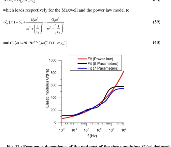
  1 2 2 2 0 2 2 2 2 1 2 1 1                _{ } _{ }     M G G G G (39) and   0    0 1 ,          _ j t   _ P G Be j t (40)

Fig. 11 : Frequency dependence of the real part of the shear modulus: G'() deduced

from the fit of G(t) by different models. Black line: power law model (Eq. (40)), redline: Maxwell model with two branches (Eq. (38)), Blue line: Maxwell Model with three

branches

Note in Eq.40 the presence of t0 in the imaginary exponential which would give a non

physical oscillation for >1/t0. In fig.14 we put t0=0 and the incomplete gamma function (1-,t0) becomes (1-) so:   1 cos 2           _{ }   G B (41)

The red curve clearly shows the two relaxation frequencies of the generalized Maxwell model, and a high frequency plateau, whereas the power law model shows a continuously increasing modulus. The addition of more than two relaxation times in the generalized Maxwell model is difficult to perform because of too many parameters which can give similar residue for different set of parameters; it can improve a little bit the fit and gives a smoother frequency dependency (blue line in Fig. 11) but in any event it remains true that both at low and high frequencies the behavior of the two models remains very different. At low frequency we find clearly a zero frequency modulus, G0 corresponding to a constant position of the indenter

after the relaxation sequence; this also confirmed by the elastic recovery of the indenter position at the end of the cycle described in Fig. 2 whereas in the power law model there is a

continuous decrease of the modulus with the frequency. Actually it is possible to add a zero frequency modulus in Eq.36 to take into account the solid like behavior, but at high frequency we find a plateau with the Maxwell model contrary to the power law model. This plateau is, of course, inherent to the Maxwell model and is imposed by the shortest relaxation time; it could be that experimentally it is not possible to test higher frequencies because the indentation velocity is limited. Actually, as can be seen in Fig. 7, we are well able to detect this plateau for indentation velocity higher than 10m/s. Furthermore, as can be seen in the insert of Fig. 10, the experimental relaxation is faster than the one predicted by the power law model, which means that this model does not well capture the physics of the relaxation process in the high frequency range. This frequency cut-off could be, for instance, related to a typical unbinding time of crosslinks, which blocks the relaxation of the actin network for smaller times [33].

4 Conclusions

In the section 2 of this paper it was shown, with the help of a comparison with FEM results on a viscoelastic solid, that a generalized Hertz theory was very well adapted to describe, not only the relaxation part, but the whole indentation curve, obtained with a spherical probe mounted on the tip of an AFM. Furthermore this equation takes into account the finite thickness of the cell with respect to the indentation depth. In the case of a Zener model, the differential equation relating the indentation to the vertical motion, z(t) of the piezoelectric transducer can be written explicitly: Eq.27 whatever the shape of z(t). For any creep function G(t), the integral equation Eq.23 can be used to obtain the parameters included in the function G(t). A proper determination of the contact between the probe and the cell and also the correction due to the viscous dissipation on the cantilever was proposed and described in Fig. 2. Based on these methods, the viscoelastic properties of Hep G2 cancer cells were obtained. It appears that high velocities of indentation reveal a short relaxation time which is generally ignored due to the use of smaller indentation velocity, This is for instance the case[2][34], where the typical time of compression was several seconds which did not allow to observe this fast relaxation time. A generalized Maxwell solid with two relaxation times is shown to rather well describe the indentation function except for the very first part of the relaxation (t<0.1s). A power law function for G(t) gives a poorer agreement in this domain and furthermore is not able to represent the solid behavior at low frequency. A tentative interpretation of this result in terms of the actin network was proposed even if it was beyond the scope of this paper which was to give a firm basis for the determination of viscoelastic functions with the help of an AFM. These results will also be used in a future work to predict the motion of magnetic nanoparticles actuated at the surface of the cell by a magnetic field. Acknowledgement

The authors thank the PACA Region and CNRS Cote d’Azur, for their financial support of the project BIOMAG and we are grateful to M. Girard from CEMEF (Sophia-Antipolis) for her help with Abaqus simulations and G.Bossis from IGMM (Montpellier) for providing the images with fluorescent microscopy.

References

[1] M. Sato, D.P. Theret, L.T. Wheeler, N. Ohshima, R.M. Nerem, Application of the Micropipette Technique to the Measurement of Cultured Porcine Aortic Endothelial

Cell Viscoelastic Properties, Journal of Biomechanical Engineering. 112 (1990) 263-268.

[2] O. Thoumine, A. Ott, Time scale dependent viscoelastic and contractile regimes in fibroblasts probed by microplate manipulation, J. Cell. Sci. 110 ( Pt 17) (1997) 2109-2116.

[3] J.P. Mills, L. Qie, M. Dao, C.T. Lim, S. Suresh, Nonlinear elastic and viscoelastic deformation of the human red blood cell with optical tweezers, Mech Chem Biosyst. 1 (2004) 169-180.

[4] S. Hénon, G. Lenormand, A. Richert, F. Gallet, A New Determination of the Shear Modulus of the Human Erythrocyte Membrane Using Optical Tweezers, Biophysical Journal. 76 (1999) 1145-1151.

[5] N. Wang, J. Butler, D. Ingber, Mechanotransduction across the cell surface and through the cytoskeleton, Science. 260 (1993) 1124-1127.

[6] G.N. Maksym, B. Fabry, J.P. Butler, D. Navajas, D.J. Tschumperlin, J.D. Laporte, et al., Mechanical properties of cultured human airway smooth muscle cells from 0.05 to 0.4 Hz, J. Appl. Physiol. 89 (2000) 1619-1632.

[7] C. Wilhelm, F. Gazeau, J.-C. Bacri, Rotational magnetic endosome microrheology: Viscoelastic architecture inside living cells, Physical Review E. 67 (2003) 061908. [8] M. Radmacher, M. Fritz, C.M. Kacher, J.P. Cleveland, P.K. Hansma, Measuring the

viscoelastic properties of human platelets with the atomic force microscope, Biophys. J. 70 (1996) 556-567.

[9] C.T. Lim, E.H. Zhou, S.T. Quek, Mechanical models for living cells--a review, J Biomech. 39 (2006) 195-216.

[10] T. Kuznetsova, M. Starodubtseva, N. Yegorenkov, S. Chizhik, R. Zhdanov, Atomic force microscopy probing of cell elasticity, Micron. 38 (2007) 824-833.

[11] A.J. Levine, T.C. Lubensky, Response function of a sphere in a viscoelastic two-fluid medium, Phys Rev E Stat Nonlin Soft Matter Phys. 63 (2001) 041510.

[12] Levine, Lubensky, One- and two-particle microrheology, Phys. Rev. Lett. 85 (2000) 1774-1777.

[13] K.L. Johnson, Contact mechanics, Cambridge Univ. Press, Cambridge, 2004.

[14] R.. Srinivasa, R.. Eswara, An FEM approach into nanoindentation on linear elastic and visco elastic characterization of soft living cells, Int J Nanotech App. (2008) 55-68. [15] E. Dimitriadis, Determination of Elastic Moduli of Thin Layers of Soft Material Using

the Atomic Force Microscope, Biophysical Journal. 82 (2002) 2798-2810.

[16] E.M. Darling, S. Zauscher, J.A. Block, F. Guilak, A Thin-Layer Model for Viscoelastic, Stress-Relaxation Testing of Cells Using Atomic Force Microscopy: Do Cell Properties Reflect Metastatic Potential?, Biophysical Journal. 92 (2007) 1784-1791.

[17] E.M. Darling, S. Zauscher, F. Guilak, Viscoelastic properties of zonal articular chondrocytes measured by atomic force microscopy, Osteoarthritis and Cartilage. 14 (2006) 571-579.

[18] V. Vadillo-Rodriguez, J.R. Dutcher, Dynamic viscoelastic behavior of individual Gram-negative bacterial cells, Soft Matter. 5 (2009) 5012.

[19] M. Balland, N. Desprat, D. Icard, S. Féréol, A. Asnacios, J. Browaeys, et al., Power laws in microrheology experiments on living cells: Comparative analysis and modeling, Phys Rev E Stat Nonlin Soft Matter Phys. 74 (2006) 021911.

[20] N. Wang, D.E. Ingber, Control of cytoskeletal mechanics by extracellular matrix, cell shape, and mechanical tension, Biophys. J. 66 (1994) 2181-2189.

[21] D.-H. Kim, E.A. Rozhkova, I.V. Ulasov, S.D. Bader, T. Rajh, M.S. Lesniak, et al., Biofunctionalized magnetic-vortex microdiscs for targeted cancer-cell destruction, Nat Mater. 9 (2010) 165-171.

[22] S.-H. Hu, X. Gao, Nanocomposites with Spatially Separated Functionalities for Combined Imaging and Magnetolytic Therapy, Journal of the American Chemical Society. 132 (2010) 7234-7237.

[23] S.M. Cook, K.M. Lang, K.M. Chynoweth, M. Wigton, R.W. Simmonds, T.E. Schäffer, Practical implementation of dynamic methods for measuring atomic force microscope cantilever spring constants, Nanotechnology. 17 (2006) 2135-2145.

[24] E. Ahassan, W. Heinz, M. Antonik, N. Dcosta, S. Nageswaran, C. Schoenenberger, et al., Relative Microelastic Mapping of Living Cells by Atomic Force Microscopy, Biophysical Journal. 74 (1998) 1564-1578.

[25] J. Alcaraz, L. Buscemi, M. Puig-de-Morales, J. Colchero, A. Baró, D. Navajas, Correction of Microrheological Measurements of Soft Samples with Atomic Force Microscopy for the Hydrodynamic Drag on the Cantilever, Langmuir. 18 (2002) 716-721.

[26] Y.-S. Chu, S. Dufour, J.P. Thiery, E. Perez, F. Pincet, Johnson-Kendall-Roberts Theory Applied to Living Cells, Physical Review Letters. 94 (2005).

[27] K. Guevorkian, M.-J. Colbert, M. Durth, S. Dufour, F. Brochard-Wyart, Aspiration of Biological Viscoelastic Drops, Physical Review Letters. 104 (2010) 218101.

[28] R. Freitas, Nanomedicine, Landes Bioscience, Austin TX, 1999.

[29] E.H. Yoffe, Modified Hertz theory for spherical indentation, Philosophical Magazine A. 50 (1984) 813-828.

[30] E. Dintwa, E. Tijskens, H. Ramon, On the accuracy of the Hertz model to describe the normal contact of soft elastic spheres, Granular Matter. 10 (2007) 209-221.

[31] J. Wilhelm, E. Frey, Elasticity of Stiff Polymer Networks, Physical Review Letters. 91 (2003) 108103.

[32] K.I. Schiffmann, Nanoindentation creep and stress relaxation tests of polycarbonate, International journal of materials research. (2006) 1199-1211.

[33] C. Broedersz, M. Depken, N. Yao, M. Pollak, D. Weitz, F. MacKintosh, Cross-Link-Governed Dynamics of Biopolymer Networks, Physical Review Letters. 105 (2010) 238101.

[34] V. Vadillo-Rodriguez, T.J. Beveridge, J.R. Dutcher, Surface Viscoelasticity of Individual Gram-Negative Bacterial Cells Measured Using Atomic Force Microscopy, Journal of Bacteriology. 190 (2008) 4225-4232.