A Framework for the Capacity Evaluation of Multihop Wireless Networks

HAL Id: hal-00371161

https://hal.archives-ouvertes.fr/hal-00371161

Submitted on 26 Mar 2009

HAL is a multi-disciplinary open access

archive for the deposit and dissemination of

sci-entific research documents, whether they are

pub-lished or not. The documents may come from

teaching and research institutions in France or

abroad, or from public or private research centers.

L’archive ouverte pluridisciplinaire HAL, est

destinée au dépôt et à la diffusion de documents

scientifiques de niveau recherche, publiés ou non,

émanant des établissements d’enseignement et de

recherche français ou étrangers, des laboratoires

publics ou privés.

A Framework for the Capacity Evaluation of Multihop

Wireless Networks

Hervé Rivano, Fabrice Theoleyre, Fabrice Valois

To cite this version:

Hervé Rivano, Fabrice Theoleyre, Fabrice Valois. A Framework for the Capacity Evaluation of

Multi-hop Wireless Networks. Ad Hoc & Sensor Wireless Networks, PKP Publishing ServicesNetwork 2010,

9 (3-4), pp.139-162. �hal-00371161�

A Framework for the Capacity Evaluation of

Multihop Wireless Networks

Herv´e Rivano

CNRS - INRIA Sophia Antipolis UNSA, 2004 route des Lucioles F-06902 Sophia Antipolis Cedex, France

Fabrice Th´eoleyre

CNRS - Grenoble Informatics Laboratory 681 rue de la passerelle, BP72 F-38402 St Martin d’H`eres, France

Fabrice Valois

INSA-Lyon, CITI F-69621, France

Abstract—The specific challenges of multihop wireles networks

lead to a strong research effort on efficient protocols design where the offered capacity is a key objective. More specifically, routing strategy largely impacts the network capacity, i.e. the throughput offered to each flow. In this work, we propose a complete framework to compute the upper and the lower bounds of the network capacity according to a physical topology and a given routing protocol. The radio resource sharing principles of CSMA-CA is modeled as a set of linear constraints with two models of fairness. The first one assumes that nodes have a fair access to the channel, while the second one assumes that on the radio links. We then develop a pessimistic and an optimistic scenarios for radio resource sharing, yielding a lower bound and an upper bound on the network capacity for each fairness case. Our approach is independent of the network topology and the routing protocols, and provides therefore a relevant framework for their comparison. We apply our models to a comparative analysis of a well-known flat routing protocol OLSR against two main self-organized structure approaches, VSR and localized CDS.

Index Terms—network capacity, multihop wireless networks,

upper and lower bounds, linear programing

I. INTRODUCTION

Ad hoc networks are spontaneous multihop topologies of wireless nodes. These networks are decentralized and should function autonomously, without any human intervention. All the nodes can be mobile, and create continuously topology changes. An ad hoc network connected to the Internet con-stitutes a so-called hybrid network. A dedicated device, the wireless access point (AP), is a gateway between the wired world and the ad hoc network.

By nature, ad hoc and hybrid networks forward traffic only via wireless links. Moreover, radio bandwidth is much lower than in wired networks, and interferences complicate the radio resource sharing. Nevertheless, multihop wireless networks with a low network capacity could become irrelevant: most applications require a minimum bandwidth to function nor-mally.

This kind of networks can be either considered in a flat manner or self-organized. Self-organization ([15]) was intro-A preliminary version of this work has been published in IEEE IWWintro-AN 2006 [17]. This work was partially supported by the European Commission project AEOLUS under contract IST-15964, project IST WIP under contract IST-27402 the French Ministry of Research project AIRNET under contract ANR-05-RNRT-012-01, project JC-OSERA, and the INRIA project ARC CARMA.

duced to tackle several key problems in multihop wireless networks (e.g. scalability, robustness, overhead) and to simplify the physical topologies. Flat approaches do not introduce any hierarchy: all the nodes must contribute equally to the network, all the radio links should be used to forward the traffic, no

organization is introduced in the network. Oppositely,

self-organizations construct a logical topology of the physical topology of the network: e.g. some radio links are pruned from the self-organization and some nodes are elected to contribute more intensively in the network management.

Although self-organization seems a promising way to man-age multihop wireless networks, the network capacity estima-tion of these soluestima-tions remains an open-problem. Indeed, a self-organization selects by nature some privileged links and nodes, and exploits them more intensively: this unbalanced se-lection impacts the network capacity. Besides, to select stable links improves the route robustness, but increases the route length which consumes more bandwidth resource. Moreover, a not-well conceived or exploited self-organization may create bottlenecks. We propose here to quantify the impact of self-organization on the network capacity.

Several articles already analyzed the asymptotical capacity of ad hoc networks [3], [4], [7], [21], [24]. However, we aim here at comparing the network capacity associated to different routing protocols for a given topology. Moreover, asymptotic studies can only give an upper bound, with an optimal MAC layer and with a fixed modeled forwarding strategy. Thus, we describe here a whole model to formulate the network capacity with a linear programming approach, interfaced with a network simulator to use directly the results of a routing protocol.

The contributions of this article are twofold:

1) We describe a complete model to extract the network capacity from any network topology. Since the paths impact the network capacity, the model directly uses the paths obtained from the routing protocol. Moreover, we present a detailed linear programming model for bandwidth sharing among interfering nodes. Our model incorporates fairness: bandwidth is fairly distributed among either interfering nodes or interfering radio links. 2) We use this model in order to compare the network capacity associated to different routing protocols. We compare in particular flat proactive and self-organized approaches. We directly use the paths computed with

different routing protocols in a discrete-event simulator. This comparison highlights the key points that must be improved to optimize the network capacity.

The article is organized as follows. The next section intro-duces hypothesis, notations and a generic model. We define formally in section III the concept of network capacity with two different objectives. Then, sections IV and V introduce the resource sharing models, for two different types of fairness (node-oriented, link-oriented), with lower and upper bounds. Section VI is dedicated to generalizing the models to arbitrary interference models and explaining the global methodology we follow for evaluating protocols. Section VII details simulations results and compare flat and self-organized routing protocols from the network capacity viewpoint. Related work on net-works capacity evaluation and routing protocol is presented in section VIII. Last section concludes this article and gives research perspectives.

II. NETWORK MODEL

We consider a wireless network modeled as a graph G(V, E) and a given routing protocol. Each vertex (V ) represents a wireless node, and an edge (E) exists between two vertices iif the corresponding nodes have a radio link with each other. We also assume that a radio link is bidirectional. We use the following notations:

• BW is the available radio bandwidth. This gives the

maximum amount of data that can be sent by a node if it is alone to transmit.

• p is a multi-hop path between a source node s and a

destination d

• f (p) is the throughput of the data sent on the path p • d(u, v) is the euclidian distance between u and v • T (u) is the total amount of traffic sent by a node u:

T (u) =!_v∈ν(u)T (u, v) + Tc(u) with

– νk(u) is the k-neighborhood of u, i.e. the set of the

nodes at most k hops far from u. ν1(u) is denoted

as ν(u) (u ∈ ν(u), ∀ k).

– ∆k(u) is the k-degree of u: ∆k(u) = |ν(u)|.

– T (u, v) is the unicast traffic on the physical radio link (u, v).

– Tc(u) is the control traffic broadcasted by u to its

neighborhood.

A. Interference models

The interferences impact the network capacity and can be modeled [8] with:

• Transmitter model: a node u can communicate with

a node v if no node w exists closer than (1 + ∆) · (range(u) + range(w)) from u

• Protocol model: the transmission (u, v) is successful if

no other node w closer than (1 + ∆)d(u, v) of v is also transmitting a packet

• Transmitter/receiver model: two radio links can be

acti-vated simultaneously if they are more than 2 hops far

• SNR: a communication (u, v) is successful if the signal

to noise ratio is larger than a threshold. The signal

Linear Program 1 Generic Model

Maximize Objective function on P

Subject to

Resource sharing constraints ∀ node u

around u

Traffic management for p _{∀ path p}

corresponds to the signal strength of u measured by v, and the noise corresponds to the ambient noise and the interference signals of all other transmitters. This model is the only one that does not assume any fixed radio range. We will use in this paper the transmitter/receiver model for all our explanations, for a sake of simplicity. However, we will

generalize in section VI-A ourLPformulation. The reader will

be able to verify that our network capacity formulation works with different interference models, and can use directly the conflict graph.

B. Linear programming models

Our linear programing models fit the generic form described

as LP 1. The objective function formalizes our definition of

the capacity. Radio resource sharing constraints are defined for each node and take into account fairness and interferences. The data flow load constraints added for each path define global constraints on the transport capacity of the network, i.e. a flow is forwarded by each intermediate node of the path.

Note that it is straightforward to write the traffic

manage-ment constraints ofLP1 from the composition of T (u, v).

C. Assumptions

In order to develop a linear model of the radio resource sharing, we need to fix some classic hypothesis on the MAC layer:

1) Perfect radio channel: we assume that the medium delivers a constant bandwidth and does not corrupt data transmissions.

2) Ideal MAC layer: no collision occurs, the bandwidth can be optimally used, and all the nodes have the same probability to reserve the radio medium

3) Bi-directional unicast communications: if a node u sends a data traffic to one of its neighbor v, v answers with an acknowledgment: any other node interfering with u or v cannot access to the medium

4) Transmitter-receiver interference model: since we as-sume communications have to be acknowledged, we block nodes interfering with the transmitter or the re-ceiver

5) Control and topology maintenance traffic is sent by u through a local broadcast. Thus, the interference model prevents all nodes interfering with the broadcaster from sending or receiving any kind of traffic

III. DEFINING THE NETWORK CAPACITY

We will first introduce two formal definitions of the network capacity: the first one deals with the classical definition of capacity and the second function introduces fairness.

A. Max-Sum function

The capacity is often described as the maximal throughput achievable in the network. Thus the objective function can be defined as: M ax  $ p∈P f (p)   (1)

In this approach, the objective is network-wide, i.e. not individual. Consequently, the network will surely privilege the radio links and nodes which create low interferences. In particular, the multihop flows will create many interferences while their bandwidth will contribute less to the objective than single hop flows. Only a few radio links will receive all the bandwidth. According to us, this objective constitutes a misinterpretation of the real capacity of a multihop wireless network for many applications. Nevertheless, this formulation gives an upper bound of the global achievable capacity.

B. Max-Min function

Fairness should be introduced. In such a case, the objective function can be formulated as:

M ax (M inp∈Pf (p)) (2)

We consider that each flow should receive the same bandwidth: multihop flows are not handicapped. The global achievable throughput will surely be inferior to the max-sum function case, since more interfering flows must cohabit. Nevertheless, we model here a multihop wireless networks with quality of service. Additionally, the fairness ratio introduced in [8] could limit unfairness among the different flows: max-min could be trivially modified to integrate this fairness ratio.

IV. NODE-ORIENTED FAIRNESS RESOURCE SHARING

A. A pessimistic scenario

To obtain a lower bound of the capacity, we model a pessimistic MAC layer in the following way. We define the interfering set of a node u as all the nodes which interfere with u (including u). A pessimistic MAC layer considers for each node its interfering set and distributes the same amount of radio bandwidth to each node. By referencing all the possible interfering sets in the network (i.e. one per node), we will define the capacity of a multihop wireless networks in a pessimistic scenario and translate it in linear constraints.

The reader can verify that this approach represents a lower bound since two radio links can be non-interfering with each other but can be referenced in the same interfering set. In this case, these links share the radio bandwidth although they can simultaneously transmit a frame without collision. For example, the radio links (A, B)/(D, E) or (K, B)/(H, I) can communicate simultaneously in the figure 1 although all these nodes are in the interfering set of C.

Fig. 1. The 2-Neighborhood of one node

Thus, a pessimistic resource sharing is achieved if the transmission of one node is blocking all its 2-neighborhood since we adopt the transmitter-receiver interference model. If the center or one of its 2-neighbors transmits a data packet, no other node in the 2-neighborhood of the center is allowed to send packets. To model a node-oriented fairness, the same bandwidth is allocated to each 2-neighbors of the center. One can notice that stopping any radio activity includes refusing any incoming connexion request, since it requires to send an acknowledgment for the received packet: it would potentially create a collision.

Control traffic is transmitted in the 1-hop neighborhood using a local broadcast: it blocks also all the 2-neighborhood. Let a node c be the center node of its 2-neighborhood. We obtain the following constraints:

• A transmission of c can only interfere with its

2-neighborhood. Thus, we assume that the bandwidth can be distributed fairly among all these contending nodes,

i.e. the 2-neighborhood of c, N2(c):

∀c, ∀u ∈ N2(c), T (u) ≤ BW

∆2(c)

(3)

Note, that for each center node c, a set of ∆2(c) equations

is given. In consequence, the bandwidth T (u) allocated

to a node u is constrained by ∆2(u) equations (one for

each possible center node).

• In the bandwidth allocated to one node, all the control

traffic and the unicast transmissions must be scheduled. Additionally, a node allocates an equal bandwidth to each of its neighbors:

∀u, ∀v ∈ N(u) − {u}, T (u, v) ≤ T (u)_{∆(u) − 1}− Tc(u) (4)

The equation (4) models a fair bandwidth sharing by a node for its neighbors, while how the radio medium bandwidth is shared among the nodes is modeled by the equation (3).

Finally, we can remark that two nodes can send data simultaneously only if they are sufficiently distant, at least 3 hops. Moreover, two nodes with different forwarding load receive the same bandwidth. This set of local constraints yields

Linear Program 2 Pessimistic model

Maximize Objective function on P

Subject to

Equation set (3) node c, the center

Equation set (4) ∀ node u

Traffic management for p ∀ path p

LP2, whose solutions lower bound the total amount of traffic

supported by the network.

B. Illustration with the pessimistic scenario on a line

We propose in this section to illustrate the previous model with the line network. This provides to the reader a step by step illustration of our models. Moreover, the line network helps to compare easily the major differences between the max-sum and max-min objectives. To simplify the explanations, the control traffic is considered null and the radio bandwidth

(BW) equal to one unit. In the max-min case, x represents the

throughput of each node. Let be the topology illustrated in figure 2. The access point is placed in the middle of the line.

The line contains 2n nodes, plus the AP.

2' 1' AP 1 2 n

n' ... ...

AP is constrained by 4 other nodes

Fig. 2. Capacity of the line (pessimistic model)

Let study the network capacity with the max-sum objective. This evaluation function will privilege uniquely the single hop flows, as described previously. Thus, it will maximize two

flows from the node 1 and 1" _{to the AP. The reader can}

remark that the access point will create the most restrictive

interference constraints.APand each of its 2-neighbors receive

1

5 of the medium bandwidth. For the node 1 (respectively

1’), the link (1,AP) (respectively (1’,AP)) receives the whole

bandwidth since only one of its radio links support traffic.

Finally, max-sum = 2

5.

Let now examine the max-min objective: AP keeps on

representing the bottleneck in the network. Let x be the traffic

sent by each node. Nodes 1 and 1" _{must receive and forward}

the traffic of the (n−1)x other nodes, and send its own traffic

to the AP. Moreover, 1 and 1" receive the same bandwidth as

in the max-sum case but here to forward the traffic of (n − 1)

nodes. We obtain the constraint 1

5 ≤ (n−1)x+x, which leads

to max-min = 1

5n

C. An optimistic resource sharing scenario

The pessimistic radio resource sharing model tends to over-estimate the interferences. Some communications could be

possible in a realistic protocol (like IEEE 802.11), but are

forbidden in our model. For example, in fig.1, the simultaneous transmissions (K → B) and (H → E) should be authorized since C has not to decipher the packets.

In consequence, we propose here an optimistic resource sharing model. For each node u, we isolate its 2-neighborhood: only these nodes can interfere with u. Then, we reference the radio links which can be activated simultaneously in this set: the attributed bandwidth will consequently be larger than in the pessimistic scenario. This approach constitutes an upper bound since we isolate one node and its 2-neighborhood. We examine node per node the resource sharing: the local constraints could lead to unfeasible global constraints. Indeed, a scheduling can be achievable locally but the combination of all the schedul-ings (one for each node) could be practically impossible: time-slots attributed to different nodes could overlap.

Let observe the behavior of the MAC layer in the two-neighborhood of a node c (the center). One neighbor, u, of the center sends a packet to v. All neighbors of u will stop any activity. When u finished the transmission, v will send a MAC acknowledgment. Thus, no neighbor of u or v is authorized to send a packet, else a collision would occur. Let

now assume that another node u" _{wants to send a packet. u}"

cannot be a neighbor of u or of v. Additionally, it must choose

a destination v" _{which is not a neighbor of u or v.}

We will now translate this behavior in linear constraints. The medium is modeled as a central entity which allocates bandwidth to each radio links, and avoids interfering links to transmit packets simultaneously. Naturally, we consider here only the radio links which must forward traffic, else we would under-estimate the available bandwidth. Thus, the radio medium distributes bandwidth among links which own to at least one path. The selection of valid transmissions is strongly correlated to the combinatorial concept of independent sets. Indeed, this contention-free communication set is an

indepen-dent set, maximal for inclusion, of the graph L1,2(L (Gc)),

defined as follows:

• G2_c is the graph of the 2-neighborhood of c.

• L(G2c) is the linegraph of G2c: it is the graph where a

vertex is associated to each edge of Gc, and an edge

between any two vertices whose corresponding edges are adjacent.

• L1,2(L(G2c)) is the graph with the same vertices as

L(G2

c), and a link between any two neighboring or

2-neighboring vertices (its 2-closure). Consequently,

L1,2(L(G2c)) represents the conflict graph of G2c.

Independent vertices (i.e. pairwise of non adjacent vertices)

of L1,2(L (Gc)) correspond to contention-free

communica-tions. An inclusion-wise maximal independent set is therefore an inclusion-wise maximal set of communications that can be activated simultaneously.

The MAC layer should achieve a fair sharing of the band-width among the maximal independent sets. Let BW (I) be the bandwidth given to the independent set I ∈ I, where I

is the set of all maximal independent sets of L1,2(L (Gc)).

BW (I) is proportional to P (I), the probability of I to be selected. The radio bandwidth can be split into:

1) The control traffic of the center: control frames are broadcasted, and broadcast frames block all the

2-neighbors of the source

2) The unicast traffic of the 2-neighborhood of the cen-ter: several unicast transmissions can be allowed, as explained above

3) The control traffic of the 1-neighbors and 2-neighbors is assumed to be contained in the unicast transmissions allocation. Since we construct an upper bound, we can consider safely that the broadcast transmissions are contained in the whole bandwidth allocated to the node for its unicast transmissions.

Consequently, the bandwidth in the neighborhood of c is finally shared as follows:

BW (I) = P (I) · (BW − Tc(c)) (5)

⇒ BW ≥ $

I∈I

BW (I) + Tc(c) (6)

The total bandwidth allocated to a communication link (u, v) is the sum of the bandwidth allocated to each inde-pendent set including (u, v), for which we deduct the control traffic of the source u:

T (u, v) ≤ $ (u,v)∈I BW (I) T (u, v) _{≤ [BW − T}c(c)] $ (u,v)∈I P (I)

Moreover,!(u,v)∈IP (I)is exactly the probability for the

communication link (u, v) to be activated by the medium. This quantity is hence denoted P (u, v) in the following:

∀(u, v) ∈ N2

2(c) ∧ v ∈ N(u),

T (u, v) _{≤ [BW − T}c(c)] · P (u, v) (7)

Unfortunately, on arbitrary network topologies, P (I) and

P (u, v) cannot be computed unless the whole set I is

known, and I has an exponential size. We therefore build a stochastic estimation of P (u, v), denoted freq(u, v) in the following. These frequencies freq(u, v) must absolutely take into account the fairness among the nodes. We propose in consequence an algorithm to construct an independent set of radio links. Initially, all the nodes can be activated (none is blocked). Let choose randomly one unblocked node u, and one of its unblocked neighbor v. This radio link (u, v) is marked as activated, and all the neighbors of u and v are marked blocked. Then, reiterate until no unblocked node exists. Finally, we obtain a list of simultaneously active radio links, i.e. an independent set in the conflict graph (algo. 1). If this algorithm is repeated n times, freq(u, v) is equal to the proportion of the cases where the link (u, v) was selected. Note that each link is directed: the link (u, v) will not receive the same amount of traffic as (v, u). Finally:

T (u, v)_{≤ (BW − T}c(c)) freq(u, v) (8)

In order to complete the model, we must take into account the control generated for routing. When the center broadcasts

Algorithm 1 Creation of independent sets with node fairness while (∃ at least one unblocked node)

do

//Chooses a random node

u_← RANDOM(unblockedNodes)

//Chooses a random neighbor

W _{← ∅}

foreach (w ∈ unblockedNodes and w ∈ N(u))

W _{← W ∪ {w}}

v _← RANDOM(W )

//Block neighboring transmissions if (W = ∅)

MARKASBLOCKED(u);

else MARKASACTIVATED(u , v); foreach (w ∈ N(u)) MARKASBLOCKED(w) endif done

Linear Program 3 Optimistic model

Maximize Objective function on P

Subject to

Equation set (8) ∀ link (u, v) ∈ E

Equation set (9) ∀ u ∈ V

Traffic management for p ∀ path p

its control traffic, all the 2-neighbors are blocked (eq. 8). Besides, a node broadcasts its traffic using the bandwidth allocated for its unicast transmissions: this constitutes an optimistic view of the control traffic distribution. We obtain consequently: $ v∈N(u) T (u, v)_{≤ freq(u, v)}$ v∈N(u) [BW − Tc(c)] − Tc(u) (9)

Besides, the bandwidth is allocated per link: a node cannot redistribute locally the bandwidth between its links. If a node chooses to redistribute the bandwidth of an unloaded link to another of its links, the interference constraints could be violated. The last optimistic aspect of this model is that the combinations of the local constraints might not yield a feasible share of the global capacity. As a matter of fact, the union of the local independent sets might not be a global independent set. In other words, the global constraints are stronger than the union of the local ones since we assume that broadcast frames do not interfere more than an unicast frame. The linear program 3 neglects this fact, yielding an upper bound on the global capacity of the network.

D. Application of the optimistic scenario on a line

Let keep on illustrating our models with the line-network scenario (fig. 3). In a first, time, we will observe the network

capacity with the max-sum. If APis the center, we obtain the

strongest constraints. The reader can verify that we obtain the following stables and frequencies:

• f req[(2", 1")] = freq[(2, 1)] = 1₂ • f req[(1,AP)] = freq[(1",AP)] =1₄

To reach the max-sum objective, only the node 1 and 1" _will

generate traffic, for the same reasons as in the pessimistic case.

Finally, max-sum = 1 4 · 2 = 1 2 2' 1' AP 1 2 n n' ... ...

1st stable center 1st stable

Fig. 3. Capacity of the line (optimistic model)

If we study the max-min objective, the neighbors of the access point will keep on constituting the bottleneck. Indeed,

1 and 1" _{generate x traffic and must forward the traffic of}

(n−1) nodes. The most-constrained set is the 2-neighborhood of the access point. The following holds:

• Through the link (1,AP) and (1",AP) must be sent the

traffic x(n)

• Through the link (i + 1, i) and (i + 1", i") must be sent

the traffic x(n − i)

The frequencies computed for the max-sum objective do not change. We have the following constraints:

• The traffic allocated to the radio link (1,AP) must be

inferior to the bandwidth multiplied by the frequency of

the link (1,AP):

x(n) _≤ 1

4 (10)

• The traffic allocated to (2, 1) must be inferior to the

bandwidth multiplied by the frequency of the link (2, 1):

x(n− 2) ≤ 1₂ (11)

Finally, max-min = 1

4n

V. LINK-ORIENTED FAIRNESS RESOURCE SHARING

Here are presented lower and upper bounds with a fairness oriented on links. While the first approach distributed fairly the bandwidth among the nodes, we chose here to distribute much bandwidth to nodes with a large number of neighbors. Consequently, we propose here to distribute fairly the band-width among the radio links which share a common interfering set. Since the previous models in section IV are very similar, we chose to present only the major differences.

Let remind that L(G) denotes the linegraph of G, i.e. the conflict graph. Let introduce the following notation:

• νk(e): the k-neighborhood in L(Ge) of one link e in

G. Each link e is directed. If we adopt the

transmitter-receiver interference model, ν2(e) is the interfering set of

e.

Linear Program 4 Pessimistic model

Maximize Objective function on P

Subject to

Equation set (12) link e

Equation set (13) ∀ link (u, v)

Traffic management for p ∀ path p

• δk(e): |νk(e)|. Similarly, δ2(e) is the number of

interfer-ing radio links

A. A pessimistic scenario

We keep on proposing a pessimistic radio resource sharing. However, instead of distributing the bandwidth to vertices, we construct for each link in the graph the set of its neighborhood in the conflict graph. If one link is active, it is potentially in conflict with each link in this set. Moreover, the same bandwidth is allocated to each link. In consequence, traffic allocated to one link f supports the following constraint:

∀e ∈ E, ∀f ∈ ν2(e),

T"(f) ≤ BW −

!

(u,x)∈ν2(e)Tc(u)

δ2(e) (12)

Additionally to data packets, a node must send control traffic. Since a broadcast packet blocks all the 2-neighborhood and we have to forbid interferences, the lower bound is achieved in duplicating a broadcast packet and sending it separately to each neighbor:

∀u, ∀v ∈ N(u) − {u}, T (u, v) ≤ T"(u, v) − Tc(u) (13)

Finally, we obtain the linear programLP4. We can remark

that the lower bounds with link-oriented and node-oriented fairness are not comparable. A different behavior of the MAC layer is modeled. Thus the capacity of the network depends on the protocol chosen to schedule concurrent medium accesses.

B. Application of the pessimistic scenario on a line

Let illustrate also the link-fairness with the line network (fig. 2 p. 4). Let focus on the interfering constraints created

by (1,AP). Since this link interferes with 4 other active links,

the bandwidth 1

5 is allocated to each of these links.

• max-sum: The node 1 and 1" sends all their traffic to the

APand receive both a bandwidth of 1. Thus, max-sum =

2 5

• max-min: The nodes 1 and 1" must send their own traffic

and forward the traffic of the line (n − 1 nodes). In

consequence, max-min = 1

5n.

C. An optimistic scenario

The upper bound with a link-oriented fairness knows less modifications. To integrate the link fairness, we just have to modify the algorithm which computes freq(u, v) (the bandwidth allocated to each link in an interfering set). The algorithm 1 (cf. page 5) must integrate the fairness when a node is chosen randomly. Consequently, instead of choosing independently one source and one destination (one of its

Algorithm 2 Creation of independent sets with link fairness while (∃ at least one unblocked link)

//Chooses a random unblocked radio link

F ← ∅

foreach (f ∈ unblockedLinks)

W _{← F ∪ {f}}

e_← RANDOM(W )

//Mark activated/blocked links

MARKASACTIVATED(e);

foreach (f ∈ ν2(e))

MARKASBLOCKED(f)

neighbors), we choose randomly one unblocked radio link. We obtain the algorithm 2.

If this algorithm is repeated n times, freq(u, v) is equal to the proportion of the cases where the link (u, v) was selected. Note that each link is here directed. Besides, each link does not receive the same amount of bandwidth: some links have potentially more interfering links and will be chosen less frequently. However, fairness among links is respected.

The remaining description of the upper bound remains

unchanged. The linear program LP3 keeps on holding, with

the new values of freq(u, v).

D. Application of the optimistic scenario on a line

Let assume that the number of nodes (n) is sufficiently large.

We will focus on the links interfering with the link (1,AP)

(fig. 3). We obtain in particular the following stables:

• stables (2", 1"), (2, 1) and (2", 1"), (3, 2)

• stable (1", AP )

• stable (1, AP )

• stable (2, 1), (2", 1")

• stables (3, 2), (1, AP ) and (3, 2), (2", 1")

Let denote freqcase1 the interfering constraints

cre-ated by (1,AP). The reader can verify in particular that

f reqcase1[(1, ap)] = 2₅ and freqcase1[(1", ap)] = 1₅. If

we take a look on the interfering constraints created by

the link (1’,AP)1_{, they are symmetric: freq}

case1(a, b) =

f reqcase2(a", b"). Finally, we obtain max − sum = 2₅.

Besides, freqcase1[(2", 1")] = 103, freqcase1[(2", 1")] = 12.

The links (2, 1) and (2"_{, 1}"_{) must transmit x(n − 1) traffic}

and the link (1, AP ) xn traffic. Thus we obtain the following constraints when we focus on the interfering constraints on

(1,AP): x(n_{− 1) ≤} 3 10 f or the links (2", 1") x(n_{− 1) ≤} 1 2 f or the links (2, 1) xn ≤ 1₅ f or the link (1", AP ) xn _≤ 3 10 f or the link (1, AP )

1_{the frequencies being denoted in this case by freqcase2}

Since we obtain symmetric constraints when we focus on the

interfering sets of (1,AP) and (1’,AP), max − min = _5n1.

VI. GENERALIZED FRAMEWORK AND METHODOLOGY

For the sake of readability, the aforesaid resource sharing equations have been described using the ”transmitter-receiver” representation of interferences [8]: two links can be activated simultaneously if they are at least 2 hops apart. However, our approach can be generalized to any binary interference model as explained in the following.

Henceforth, these linear models define a framework for evaluating the transport capacity provided by a given routing strategy on a network topology. To complete the framework, we describe the process articulating a discrete event simulation with the linear models as well as the methodology we have followed exploiting the framework.

A. Generalizing to arbitrary interference model

Even though the linear equations introduced in the pre-ceding sections consider a 2 hop distance binary interference model like the ”transmitter-receiver” representation, the ap-proach can be generalized to any other binary interference model.

In particular, a binary interference model is given as a conflict graph describing the pairwise incompatibilities among the radio link: two links can be activated simultaneously if and only if they are not adjacent in the conflict graph [12].

That gives a straightforward way to generalize all the models for bandwidth sharing. For instance, we can extend the link fairness equation (eq. 12). The 2-neighborhood of an

edge e, ν2(e), is replaced by the neighborhood of e in the

conflict graph. Equivalently, the number of interfering links,

δ2(e), is replaced by the degree of e in the conflict graph. The

node fairness equations are generalized similarly. Two nodes are claimed as interfering if and only if they are either adjacent in the network or incident to a pair of links that are adjacent in the conflict graph. The computations and equations stay.

B. Network capacity evaluation methodology

The framework we are developing aims at evaluating the capacity provided by a routing protocol. The linear models need to be given the topology of the network, the paths built by the routing protocol, and the control traffic generated by the protocol. In order to generate these data in a realistic manner, we run a discrete event simulation of a mobile network running the protocol. We define the framework by the following process:

1) A topology of x nodes is simulated (in our case,

x_{∈ [20..60], with a degree of 10. Nodes are randomly}

located in a squared simulation area).

2) The routing protocol is simulated and gives the over-heads and paths (the paths depends on the traffic pat-tern).

3) The constraints modeling the radio resource sharing are extracted from the radio topology.

5) The capacity is computed from the list of constraints and the objective functions (cf. section III)

In our implementation, the simulations are done using

OPNETModeler [13] while the linear programs are solved with

CPLEX [5]. For the sake of reproducibility of experiments,

the built of the linear programs is distributed as a part of the

MASCOPTlibrary [11].

Our objective is to estimate the capacity inherent to different routing protocols. To reach this goal, the behavior of some routing protocols were simulated. We have also implemented two traffic patterns: in an ad-hoc network, all the possible paths are computed (Any-To-Any), in an hybrid network, only paths toward one Access Point are computed (Any-To-One).

To have a representative view of the different routing ap-proaches, we have simulated the three following major routing protocols.

• OLSR is relevant to represent the behavior of flat routing

protocols computing (or approximating) shortest paths routing.

• Localized-CDS: all the traffic is sent through a meshed

backbone provided by [22]

• VSR & SOMoM: in the ad hoc approach (VSR version),

paths use a cluster topology. In the hybrid approach of

VSR (denoted asSOMoMversion), paths use uniquely the

tree backbone topology, for which the AP represents the root [18], [19].

Our framework allows to quantify the network capacity of these different routing schemes with a neutral point of view in the sense it relies only on the structure of the paths and the volume of the control traffic. In the following section, we present the results of our simulations. We assume that the radio bandwidth is normalized to 1. First, we give general remarks on the evolution of the capacity according to network size. Then, we compare the capacities of different routing protocols in an ad-hoc and hybrid network.

VII. RESULTS

A. General evolution of the capacity

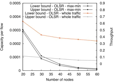
First, we evaluate the general evolution of the capacity in multihop wireless networks with the link-oriented fairness, which maximizes the minimum capacity allocated to each flow in a flat network (fig. 4). In a multihop wireless network, a network with n nodes comprises n(n − 1) paths. With a flat routing protocol, we can remark that the bandwidth per flow decreases when the number of nodes increases: the number of flows grows, and this creates more contention. Consequently, the bandwidth allocated to each flow will surely decrease, corroborating the results of [3]. Oppositely, the total aggregated capacity (the sum of traffic of individual flows) remains constant. Indeed, many flows will with high probability pass through the center of the network since OLSR uses shortest paths. Consequently, almost all the flows are limited by the same interfering set, which leads to a constant aggregated capacity. The center will represent a bottleneck,

0 0.0001 0.0002 0.0003 0.0004 0.0005 20 25 30 35 40 45 50 55 60 0 0.1 0.2 0.3 0.4 0.5 0.6 0.7 0.8 0.9

Capacity per flow

Throughput

Number of nodes Lower bound - OLSR - max-min Upper bound - OLSR - max-min Lower bound - OLSR - whole traffic Upper bound - OLSR - whole traffic

Fig. 4. Comparison of the objective functions in an ad-hoc network using flat routing (link-oriented fairness)

and limit the spatial frequency re-utilization. Finally, we can note that the optimistic and the pessimistic resource sharing present a very close capacity.

B. Ad-hoc networks

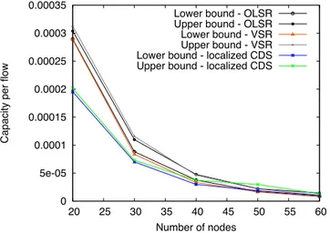
We start by maximizing the global network throughput using the max-sum objective (fig. 5). This evaluation doesn’t ensure fairness among the flows: short paths will be privileged since they create less radio interferences. Thus, the global capacity does not decrease when the network cardinality increases. We can even remark that with the optimistic bandwidth sharing, the global capacity increases. Indeed, the network size increases since the degree is maintained constant. Thus, more flows can be activated simultaneously since they are spatially distributed. Oppositely, the pessimistic resource shar-ing tends to over-estimate interferences, and limit the spatial re-utilization in small networks. Besides, we can remark that OLSR and VSR present a very close capacity, whatever the objective function is while the capacity of Localized-CDS protocol remains much lower. In conclusion, in an ad hoc network, a self-organization scheme does not impact severely the capacity since OLSR and VSR offer similar throughputs. Then, we investigate the capacity with a link-oriented fair-ness but with the max-min objective (fig. 6). We can remark for the same reason as described previously that the capacity decreases when the number of nodes increases. We can also verify that OLSR and VSR offer the same capacity when we ensure fairness among the different flows. The backbone of Localized-CDS routing keeps on constituting a bottleneck and impact severely on the capacity.

We also evaluated the capacity with the node-oriented fairness (fig. 7). While the capacity of OLSR and VSR remain unchanged, Localized-CDS routing suffers from the node-oriented fairness. Indeed, backbone clients and backbone members receive the same amount of bandwidth although backbone nodes must forward more packets. Thus, link-oriented fairness would improve the capacity by privileging

0 1 2 3 4 5 6 20 25 30 35 40 45 50 55 60 Aggregated Capacity Number of nodes Lower bound - OLSR Upper bound - OLSR Lower bound - VSR Upper bound - VSR Lower bound - localized CDS Upper bound - localized CDS

Fig. 5. Capacity of an ad-hoc network with the max-sum objective

(link-oriented fairness) 0 5e-05 0.0001 0.00015 0.0002 0.00025 0.0003 0.00035 20 25 30 35 40 45 50 55 60

Capacity per flow

Number of nodes Lower bound - OLSR Upper bound - OLSR Lower bound - VSR Upper bound - VSR Lower bound - localized CDS Upper bound - localized CDS

Fig. 6. Capacity of an ad-hoc network with the max-min objective

(link-oriented fairness)

nodes that must forward traffic from a lot of neighbors

C. Hybrid networks

Finally, we study the capacity of an hybrid network with the max-min objective and the link-oriented fairness (fig. 8). In an hybrid network, the Access Point constitutes either the destination or the source of each flow. Thus, in a network with n nodes, exactly 2n flows exist. Consequently, the capacity per flow is much higher than in a multihop wireless

network (fig. 8). OLSR offers an higher capacity thanSOMoM

and Localized-CDS protocol: the access point represents the bottleneck of the hybrid network, but the flat routing protocol distributes efficiently the path. The backbone of

Localized-CDS protocol presents an higher throughput than SOMoM: the

first one seems more efficient in hybrid networks to distribute the load among the backbone nodes.

In hybrid networks, a self-organization protocol seems to offer a degraded capacity compared to a flat routing protocol. Thus, an efficient backbone construction protocol optimizing

0 5e-05 0.0001 0.00015 0.0002 0.00025 0.0003 0.00035 20 25 30 35 40 45 50 55 60

Capacity per flow

Number of nodes Lower bound - OLSR Upper bound - OLSR Lower bound - VSR Upper bound - VSR Lower bound - localized CDS Upper bound - localized CDS

Fig. 7. Capacity of an ad-hoc network with the max-min objective (node-oriented fairness)

the load distribution among the neighbors of the AP must be proposed. 0 0.002 0.004 0.006 0.008 0.01 0.012 0.014 20 25 30 35 40 45 50 55 60

Capacity per flow

Number of nodes Lower bound - OLSR Upper bound - OLSR Lower bound - VSR Upper bound - VSR Lower bound - localized CDS Upper bound - localized CDS

Fig. 8. Capacity of an hybrid network with the max-min objective

(link-oriented fairness)

VIII. RELATEDWORK

The authors of [3] presented a pioneering work to extract the network capacity based on the protocol interference model (see section II-A). They defined the network capacity as the aggregated achievable throughput, as considered in this paper. The authors defined spatial and scheduling constraints and proved that even if nodes choose an optimal radio range, the

capacity per node does not exceed O'_√1

n

(

, with n being the number of nodes.

Several articles extended this work to deal with hybrid networks [7], [10], [24], broadcast [9] and multicast [21]. [4] proposes to use simulations to extract the network capacity. Finally, [16] proposes to optimize greedily the AP placement but interference models are simplistic: the throughput is as-sumed to be proportional to the path length.

Thus, none of these propositions was conceived to compare the network capacity achieved with different routing protocols.

A. LP formulation of the network capacity

The authors of [6] used linear programing to model the capacity of ad hoc networks. Interferences, radio topology and resource sharing are translated in linear constraints. However, the complexity resides in the capacity estimation of each edge. The authors constructed the conflict graph with the protocol interference model. They estimated that the maximum throughput is achieved when a scheduling is contained in an independent set of the radio links in the conflicts graph. Since to reference exhaustively all the maximum independent sets (MIS) is NP hard, the authors propose to find a sufficiently large number of MIS. Then, they proposed a scheduling which allocates a slot time t to each MIS (t ∈ [0..1], the radio capacity is equal to one unit) and maximizes the capacity. Consequently, the authors do not try to model fairness in the radio resource sharing, contrary to our approach described above.

[8] proposed a scheduling of radio links so that two links activated simultaneously never interfere with each other. The authors proposed a greedy allocation algorithm after an or-dering of radio links by their euclidean distance. However, they tend to under-estimate the capacity: bandwidth is shared equally among one edge and each of its interfering edges, even if some of these links do not interfere with each other and could transmit a packet simultaneously. Our capacity estimation proposes a finer evaluation of the local resource sharing in studying more precisely the interference interactions among the 2-neighborhood of a node.

B. Routing in multihop wireless networks

Routing protocols are very closely related to the capacity of ad hoc networks. With different paths, a network will achieve dissimilar throughputs. Bottlenecks should be avoided, and the load harmoniously distributed to improve frequency spatial re-utilization.

To construct paths in a multihop wireless networks, two main strategies exist. In the first one, the network is considered flat [14], [2]. In this paper, we cope with OLSR since we consider it is representative of the flat approach to compute paths in multihop wireless networks. OLSR limits the broad-cast storm problem by using Multi-Point Relays to limit the overhead due to topology packets. In the second approach, the network is self-organized before routing takes place. For instance, some approaches [23], [22] aim at constructing a backbone (more precisely, a Connected Dominating Set) to optimize the flooding of topology packets. Consequently, packets are routed through the backbone, and a bottleneck could appear. Besides, VSR[19] uses the cluster and backbone topology of [20] for routing: each node executes a proactive routing inside its cluster while a reactive protocol uses the stable cluster topology to route packets between different clusters.

Since a self-organization is a subset of the radio topology, it should avoid the apparition of bottlenecks. In other words, we have to verify that self-organization does not reduce the network capacity compared to flat approaches. Thus, we provided in this article models and the associated framework to compare the network capacity for any routing protocol.

IX. CONCLUSION AND FUTURE WORK

This paper focuses on generic methods for evaluating the capacity of multihop wireless networks. Our approach consists in modeling radio resource sharing principles of CSMA-CA protocols as a set of linear constraints. We propose two MAC layer fairness models. One assumes a fair bandwidth repartition among the interfering nodes, while the other one distributes fairly the bandwidth among the radio links. For each of these fairness models, we propose a pessimistic and an optimistic scenario of the spatial-reutilization of the radio resources. This framework is generic, not related to a particular topology or routing algorithm: we can compare quantitatively different routing strategies. We conclude that self-organization protocols can have a negligible impact on the network capacity with a traffic pattern any-to-any. However, efforts have to be done for self-organizations based routing in a many-to-one traffic pattern.

In the close future, we plan to pursue our comparison campaign by including the other main flat routing proto-cols (AODV, DSR, DSDV), even though we conjecture that their performances should theoretically be similar to those of OLSR. We are also interested in evaluating multi-path routing protocols [1], since they have been proposed for improving the throughput of the network. In this article, we obtained the network capacity of a given routing algorithm and its associated topology. We want now adopt the inverse approach: how to conceive a routing algorithm which optimizes the network capacity?

REFERENCES

[1] J. L. Bredin, E. D. Demaine, M. Hajiaghayi, and D. Rus. Deploying

sensor networks with guaranteed capacity and fault tolerance. In

International Symposium on Mobile Ad Hoc Networking & Computing (MOBIHOC), pages 309–319, Urbana-Champaign, USA, May 2005.

ACM.

[2] T. Clausen and P. Jacquet. Optimized link state routing protocol (OLSR). RFC 3626, IETF, October 2003.

[3] P. Gupta and P. R. Kumar. The capacity of wireless networks. IEEE

Transactions on Information Theory, 46(2):388–404, March 2000.

[4] H.-Y. Hsieh and R. Sivakumar. Performance comparison of cellular and multi-hop wireless networks: a quantitative study. In SIGMETRICS, pages 113–122, Cambridge, USA, June 2001. ACM.

[5] ILOG CPLEX. http://www.ilog.com/products/cplex/ index.cfm (v7.5).

[6] K. Jain, J. Padhye, V. Padmanabhan, and L. Qiu. Impact of interference on multi-hop wireless network performance. In International Conference

on Mobile Computing and Networking (MOBICOM), pages 66–80, San

Diego, USA, September 2003. ACM.

[7] U. C. Kozat and L. Tassiulas. Throughput capacity of random ad hoc networks with infrastructure support. In International Conference on

Mobile Computing and Networking (MOBICOM), pages 55–65, San

Diego, USA, September 2003. ACM.

[8] A. Kumar, M. Marathe, S. Parthasarathy, and A. Srinivasan. Algorithmic aspects of capacity in wireless networks. ACM SIGMETRICS

[9] X.-Y. Li, J. Zhaot, Y.-W. Wu, S.-J. Tang, X.-H. Xu, and X.-F. Mao. Broadcast capacity for wireless ad hoc networks. In International

Conference on Mobile Ad Hoc and Sensor Systems (MASS), Atlanta,

USA, September 2008. IEEE.

[10] B. Liu, Z. Liu, and D. Towsley. On the capacity of hybrid wireless networks. In INFOCOM, volume 3, pages 1543–1552, San Francisco, USA, April 2003. IEEE.

[11] Mascopt Library. http://www.inria.fr/sophia/teams/mascotte/mascopt/. [12] C. Molle, F. Peix, and H. Rivano. An optimization framework for the

joint routing and scheduling in wireless mesh networks. In Proc. 19th

IEEE International Symposium on Personal, Indoor and Mobile Radio Communications (PIMRC’08), Cannes, France, Sept. 2008.

[13] OPNET Modeler. http://www.opnet.com (v8.1a), bethesda, md. [14] C. E. Perkins, E. M. Belding Royer, and S. R. Das. Ad hoc on-demand

distance vector (AODV) routing. RFC 3561, IETF, July 2003. [15] C. Prehofer and C. Bettstetter. Self-organization in communication

networks : principles and design paradigm. IEEE Communications

Magazine, 43(7):78–85, July 2005.

[16] L. Qiu, R. Chandra, K. Jain, and M. Mahdian. Optimizing the placement of integration points in multi-hop wireless networks. In International

Conference on Network Protocols (ICNP), Berlin, Germany, October

2004. IEEE.

[17] H. Rivano, F. Theoleyre, and F. Valois. Capacity evaluation framework and validation of self-organized routing schemes. In International

Workshop on Wireless Ad-hoc and Sensor Networks (IWWAN),

New-York, USA, June 2006. IEEE.

[18] F. Theoleyre and F. Valois. Mobility management in multihops wireless access networks. In Personal Wireless Communications (PWC), pages 146–153, Colmar, France, August 2005. IFIP.

[19] F. Theoleyre and F. Valois. Virtual structure routing in ad hoc networks. In International Conference on Communications (ICC), volume 2, pages 3078–3082, Seoul, Korea, May 2005. IEEE.

[20] F. Theoleyre and F. Valois. Self-organization through a virtual structure for hybrid networks. Ad Hoc Networks, 6(3):393–407, May 2008. [21] Z. Wang, H. R. Sadjapour, and J. Garcia-Luna-Aceves. A unifying

perspective on the capacity of wireless ad hoc networks. In INFOCOM, pages 753–761, Phoenix, USA, May 2008. IEEE.

[22] J. Wu and F. Dai. Distributed dominant pruning in ad hoc wireless networks. In International Conference on Communications (ICC), pages 353–357, Anchorage, USA, May 2003. IEEE.

[23] J. Wu and H. Li. A dominating-set-based routing scheme in ad hoc wireless networks. Telecommunication Systems Journal, 18(1-3):63–83, September 2001.

[24] A. Zemlianov and G. De Veciana. Capacity of ad hoc wireless

networks with infrastructure support. IEEE Journal on Selected Areas