HAL Id: hal-01757139
https://hal.sorbonne-universite.fr/hal-01757139
Submitted on 3 Apr 2018
HAL is a multi-disciplinary open access
archive for the deposit and dissemination of
sci-entific research documents, whether they are
pub-lished or not. The documents may come from
teaching and research institutions in France or
abroad, or from public or private research centers.
L’archive ouverte pluridisciplinaire HAL, est
destinée au dépôt et à la diffusion de documents
scientifiques de niveau recherche, publiés ou non,
émanant des établissements d’enseignement et de
recherche français ou étrangers, des laboratoires
publics ou privés.
Distributed under a Creative Commons Attribution| 4.0 International License
On the Occurrence of Thermal Nonequilibrium in
Coronal Loops
C. Froment, F. Auchère, Z. Mikić, G. Aulanier, K. Bocchialini, Eric Buchlin,
J. Solomon, E. Soubrié
To cite this version:
C. Froment, F. Auchère, Z. Mikić, G. Aulanier, K. Bocchialini, et al.. On the Occurrence of Thermal
Nonequilibrium in Coronal Loops. The Astrophysical Journal, American Astronomical Society, 2018,
855 (1), pp.52. �10.3847/1538-4357/aaaf1d�. �hal-01757139�
On the Occurrence of Thermal Nonequilibrium in Coronal Loops
C. Froment1,2,3 , F. Auchère3 , Z. Mikić4 , G. Aulanier5 , K. Bocchialini3 , E. Buchlin3 , J. Solomon3, and E. Soubrié3,6
1
Rosseland Centre for Solar Physics, University of Oslo, P.O. Box 1029 Blindern, NO-0315 Oslo, Norway;clara.froment@astro.uio.no
2
Institute of Theoretical Astrophysics, University of Oslo, P.O. Box 1029, Blindern, NO-0315, Oslo, Norway 3
Institut d’Astrophysique Spatiale, CNRS, Univ. Paris-Sud, Université Paris-Saclay, Bât. 121, F-91405 Orsay, France 4
Predictive Science, Inc., San Diego, CA 92121, USA 5
LESIA, Observatoire de Paris, PSL Research University, CNRS, Sorbonne Universités, UPMC Univ. Paris 06, Univ. Paris Diderot, Sorbonne Paris Cité, 5 place Jules Janssen, F-92195 Meudon, France
6
Institute of Applied Computing & Community Code, Universitat de les Illes Balears, E-07122 Palma de Mallorca, Spain Received 2018 January 11; revised 2018 February 9; accepted 2018 February 11; published 2018 March 7
Abstract
Long-period EUV pulsations, recently discovered to be common in active regions, are understood to be the coronal manifestation of thermal nonequilibrium (TNE). The active regions previously studied with EIT/Solar and Heliospheric Observatory and AIA/SDO indicated that long-period intensity pulsations are localized in only one or two loop bundles. The basic idea of this study is to understand why. For this purpose, we tested the response of different loop systems, using different magnetic configurations, to different stratifications and strengths of the heating. We present an extensive parameter-space study using 1D hydrodynamic simulations(1020 in total) and conclude that the occurrence of TNE requires specific combinations of parameters. Our study shows that the TNE cycles are confined to specific ranges in parameter space. This naturally explains why only some loops undergo constant periodic pulsations over several days: since the loop geometry and the heating properties generally vary from one loop to another in an active region, only the ones in which these parameters are compatible exhibit TNE cycles. Furthermore, these parameters(heating and geometry) are likely to vary significantly over the duration of a cycle, which potentially limits the possibilities of periodic behavior. This study also confirms that long-period intensity pulsations and coronal rain are two aspects of the same phenomenon: both phenomena can occur for similar heating conditions and can appear simultaneously in the simulations.
Key words: Sun: atmosphere– Sun: corona – Sun: UV radiation
1. Introduction
Solving the coronal heating problem remains one of the biggest challenges in astrophysics. How can the tenuous plasma that constitutes the highest layer of the solar atmosphere be maintained at temperatures two orders of magnitude higher than that of the solar surface? One of the fundamental facets of this problem is to determine the spatial and temporal distribution of the heating.
Thermal nonequilibrium (TNE) is a phenomenon that can occur in the solar atmosphere when the heating is highly stratified (e.g., Mendoza-Briceño et al. 2005; Karpen & Antiochos 2008; Mok et al. 2008,2016; Antolin et al. 2010; Susino et al. 2010; Lionello et al. 2013). This particular
localization of the heating produces chromospheric evaporative upflows that supply the coronal structure with dense and hot material. A thermal runaway is eventually triggered when the radiative losses overcome the limited heating at coronal heights. Condensations are formed locally in the corona and fall down to the loop footpoints along the magneticfield lines. Furthermore, if the heating is quasi-steady, i.e., with a high heating frequency compared to the typical cooling time, this phenomenon can be cyclic. Such a system has no existing thermal equilibrium and will undergo evaporation and condensation cycles with periods of a few hours. This highly nonlinear behavior is what we call TNE. The limit cycle
solutions in coronal loops were first explored by Kuin & Martens(1982).
TNE has received increasing interest in recent years. The thermal runaway triggered by a local excess of density and leading to cool condensations is one of the standard explanations for the existence of cool materials in the corona. Such catastrophic cooling events can, for example, end up in the formation of prominences (Antiochos & Klimchuk
1991; Antiochos et al. 1999, 2000; Karpen et al. 2006; Xia et al.2011,2014) or coronal rain (Schrijver2001; Müller et al.
2003, 2004, 2005; De Groof et al. 2004, 2005; Antolin et al. 2010,2012; Vashalomidze et al. 2015). Coronal rain is
widely observed in off-limb active regions (e.g., Antolin & Rouppe van der Voort 2012; Antolin et al. 2015), even if a
proper quantification of the proportion of loops experiencing episodes of coronal rain is still lacking.
Nevertheless, the widespread existence of TNE in loops, and, consequently, the widespread contribution of quasi-steady footpoint heating, has been questioned(Klimchuk et al.2010).
However, recent modeling studies have shown that the role of TNE in the dynamics of loops may need to be revisited (Lionello et al.2013,2016; Mikić et al.2013; Winebarger et al.
2014; Mok et al. 2016). These modeling studies support the
idea that TNE is probably common in coronal loops, with two main types of condensations involved. Mikić et al. (2013) in
particular suggest that different regimes of TNE cycles could exist in loops. They differentiate cycles with complete condensations (CCs) where the temperature, locally in the corona, drops to chromospheric temperatures to form dense (up to ~1017m-3) and cool blobs, related to the observed coronal rain, and cycles with incomplete condensations (ICs).
© 2018. The American Astronomical Society.
Original content from this work may be used under the terms of theCreative Commons Attribution 3.0 licence. Any further distribution of this work must maintain attribution to the author(s) and the title of the work, journal citation and DOI.
For this other regime of TNE, the temperature stays at coronal temperatures, and the density remains relatively low (~ ´5 10 m15 -3). These two different regimes of evaporation and condensation cycles are obtained with different combina-tions of parameters of the loop geometry and of the heating strength and spatial distribution.
The early statistical study of long-period intensity pulsations by Auchère et al. (2014) brings new impetus to this debate.
Using 13 yr of data in the 195Åchannel of the Extreme-ultraviolet Imaging Telescope (EIT; Delaboudinière et al.
1995) on board the Solar and Heliospheric Observatory
(Domingo et al. 1995), the authors found that at least half of
the active regions likely undergo these intensity pulsations with periods ranging from 2 to 16 hr. In particular, these pulsations are very common in coronal loops. They have also been observed with the coronal channels of the Atmospheric Imaging Assembly (AIA; Boerner et al. 2012; Lemen et al.
2012) on board the Solar Dynamics Observatory (SDO; Pesnell
et al. 2012), during the first 6 yr of the AIA archive
(Froment2016).
Froment et al.(2015) studied three examples of such events
in detail, with periods of 3.8, 5.6, and 9.0 hr. The authors concluded that these events are related to TNE cycles. This study was focused on the thermal structure evolution of these loops, using simultaneously the six coronal passbands of AIA. The authors used both differential emission measure, with diagnostics developed by Guennou et al.(2012a,2012b,2013),
and time lag analysis, using the same method as presented in Viall & Klimchuk(2012). Auchère et al. (2016a) have recently
critically reexamined and confirmed the statistical significance of the detections used in Froment et al. (2015). Furthermore,
the pulse-train nature of the observed signals highlighted by Auchère et al. (2016b) reinforced the conclusion that TNE is
the cause of the long-period intensity pulsations observed. Finally, we recently conducted a modeling study in order to compare directly the simulations with these observations. In this 1D hydrodynamic simulation study(Froment et al.2017, hereafter PaperI), we showed that with a highly stratified and
steady heating we can reproduce the main characteristics (average behavior integrated along the line of sight and long-term temporal variations) of the thermal behavior of the loop bundle of event 1 studied in Froment et al.(2015).
As already mentioned in Froment et al.(2015), in the active
regions where long-period intensity pulsations are detected, only one loop bundle (or in some rare cases two) shows this kind of behavior. The automatic detection algorithm used may have missed events owing to the rather strict detection thresholds that we used. It is also likely that some events are missed by the Fourier detection if they are not strictly periodic. Furthermore, the background and foreground emission could mask the time-varying signal in certain cases. However, some properties, such as the geometry of the magneticfield lines and the heating characteristics, could favor the TNE cycles for only some loop bundles. In the present paper we explore the sensitivity of TNE occurrence as a function of the heating strength and stratification, for several loop geometries.
The heating parameters used in the simulation presented in PaperI have been chosen among hundreds of heating combinations tested for a single loop geometry, which corresponds to a pulsating loop bundle observed with AIA. We present here an extensive parameter-space study that justifies this particular choice. To extend our analysis, we also
pick another loop geometry, corresponding to a nonpulsating loop from a neighboring region, and use a semicircular one as a test sample to do the same analysis and thus test the influence of the loop geometry.
This parameter-space exploration is presented in Section2. In Section3we discuss our results regarding the occurrence of TNE cycles within the parameter space explored. Then, in Section 4 we examine the properties of the different types of loop systems produced in our simulations(with TNE or not) in relation to the observed loop properties. Finally, we summarize our results in Section5.
2. Parameter-space Scan
For this parameter-space study, we use the same 1D hydrodynamic code as in Mikić et al. (2013) and in PaperI. The 1D description is particularly suited for this kind of study, as multiple configurations of loops can be easily tested. The loop geometries used in these simulations, except for one loop (loop A; see Section 2.2), are from the linear force-free field
(LFFF) extrapolations presented in Section2.1 of PaperI. These extrapolations are made using magnetograms from the Helioseismic and Magnetic Imager(HMI; Scherrer et al.2012)
corresponding to the active regions of event1 of Froment et al. (2015), i.e., NOAAAR11499, and NOAAAR11501, a
smaller adjacent active region. Some selected extrapolated field lines are presented in Figure 1. We detected intensity pulsations (with a period of 9.0 hr) in a large loop bundle of NOAAAR11499, with a very clear signal; the probability that this detection was caused by noise is 1.7×10⁻⁸ (Auchère et al.2016a). This area is delineated by the orange contour in
Figure1.
Figure 1.Somefield lines extrapolated for NOAA AR 11499 and 11501 with an LFFF model. Contours of magnetic field (Bz at z= 0) from the HMI
magnetogram are in light red for positive values and in light blue for negative ones for±30 G. The AIA 171 Åimage and the magnetogram are both taken on 2012 June 06 at 23:12 UT. The orange contour delimits the area of the pulsations(9.0 hr of period) detected in the 335 Åpassband of AIA (see Figure 4 in Froment et al. 2015), for a sequence of data between 2012 June 05
11:14UT and 2012 June 08 11:16UT. The red field lines match this contour. The white arrows indicate the loopsB and C chosen for the parameter-space study. See Section2.1 of Paper I for further details regarding these extrapolations.
In the field of view presented in Figure 1, outside of the orange-contoured bundle, no other loop bundle shows a long-period pulsating behavior. The evolution of the pulsating loops has been followed from 2012 June 03 18:00UT to 2012 June 10 04:29UT using AIA data.
2.1. Method and Parameters Explored
We choose to focus on three different loop geometries and to scan various heating configurations for these loops. In addition to the loop geometry that matches the pulsating loop bundle already used in PaperI (noted here as loop B), we use a
semicircular geometry as a control sample (loop A), and we picked another loop geometry from the LFFF extrapolation that matches with a nonpulsating loop bundle as observed with AIA (loop C). The field lines corresponding to loopB and loopC, and matching visible loop bundles in the 171ÅAIA image, are indicated in Figure1. LoopA is an ad hoc loop and is therefore not present in the field of view.
The 1D hydrodynamic simulations are made using the same initial conditions and assumptions as in PaperI(see description in
Section2.2). The only difference here is that instead of using the
Spitzer thermal conductivity as in PaperI, we use an option present in the code(Mikić et al.2013) to artificially broaden the
transition region at low temperatures. This modification of k allows us to reduce the steep gradients below a cutoff temperature (chosen as Tc=250,000 K here) with a minimal effect on the
coronal solutions, as described in Lionello et al.(2009) and Mikić
et al.(2013). In that way we can afford to use bigger mesh cells
and thus fewer mesh points, i.e., 10,000 points, than in Paper I. This technique is particularity suited for this study, since we wish to scan a large area of the space of parameters. Some of the runs presented in this paper were repeated with the classic, unmodified, Spitzer conductivity using more mesh points (typically 100,000 points). It is the case for the particular simulations that we choose to present in detail in Section4(see Figure16) and some examples
presented in Froment(2016). The overall pattern is not affected by
this technique, but some differences related to the precise nature of condensations can appear between the simulations using the Spitzer thermal conductivity and the ones using modified conductivity.
We choose a simple heating function that can be tuned with three free parameters. This heating function is the same as the one used in PaperI(see Equation (2)):
= + - l + - - l
( ) ( ( ) ( ) ) ( )
H s H H e g s e g L s , 1
0 1 1 2
whereg s( )=max(s- D, 0 and) Δ=5 Mm is the thickness of the chromosphere, where the heating is constant.
H(s) is the volumetric heating rate, expressed in W m−3. H0
is the value to which H(s) tends at the apex, and(H0+H1)is the value of the heating in the chromosphere.λ1andλ2are the
scale lengths for the energy deposition at the eastern and western leg of the loop, respectively.
For each loop geometry we test several values of H1,λ1, and
λ2. We choose tofix the H0value for each loop geometry, to a
value that allows us to obtain a static loop(we set H1=0 to
use a uniform heating) with an apex temperature around 1MK. For each loop geometry, we explored values of H1 in
increments of a factor of 2. In that way we can easily compare the simulations. Note that the value of the factor itself is arbitrary. For each value of H1explored, we test a large set of
combinations ofλ1andλ2, specified in percentage of the total
length L of each loop. The scan cube is then (H1,λ1,λ2).
For each simulation, we can define the heat flux, i.e., the total heat that the loop receives over its length, normalized to thefirst loop footpoint cross-sectional area:
ò
= ( )´ ( ) [ - ] ( ) Q A H s A s ds 1 W m , 2 L 0 0 0 2with A(s) the cross-sectional area of the loop, which is~1 B s( ). As we will see in Section2.2(Figures2and3), the magnetic field
strength is similar at both ends of each loop geometry chosen. The heat flux normalized at the second footpoint, Q1, is thus
always similar to Q0. We thus only consider this latest value. The
Q0 heat flux value does not give information about the
asymmetry of the heating. However, looking at Equations (1)
and (2), we can see that the heating in a leg will be dominant
when the scale height of energy deposition is larger, and the more the loop area expansion is important in this leg.
It is worth noting that the way we choose to explore the parameter space of the heating strength and stratification implies that Q0changes between two slices through the scan cube, i.e.,
between simulations with the same stratification (λ1,λ2) but with
different values of the heating at the footpoints(H1). Indeed, Q0
changes from one simulation to another. We could have chosen a different parameterization, fixing Q0 instead of H1 for each
exploration of λ1 and λ2. However, we confirmed that this
different parameterization did not change our conclusions. In addition, whatever the parameterization, since Q0 and H1 are
linked, the results can be explored at Q0constant. We tested as
well an alternate way of creating asymmetry in the heating along the loop by applying a different amount of heating at each footpoint. We verified that this did not change the conclusions of this paper either.
2.2. Loop Geometries
In Figure2, we present the loop geometry of loopA, the test case semicircular geometry we use for the first set of
Figure 2.Geometry profiles for loopA. This loop geometry is not from the LFFF extrapolations. Top left: loop profile, altitude in Mm of each point along the loop. Top right: normalized acceleration of the gravity projected along the loop(see Equation (1) of PaperI). Bottom left: strength of the magnetic field
B(s) in Gauss. Bottom right: loop expansion given by the evolution of the cross-sectional area A(s), normalized to the first footpoint.
simulations. In Figure 3, we present the loop geometry of loopsB andC, which are from two field lines extracted from the LFFF extrapolations of the active regions presented in Figure1. These loop geometries, even if from singlefield lines, are selected to model the behavior of the corresponding loop bundles. When we compare the simulations with observations, a simulated loop represents the average behavior of a loop bundle, whose individual threads all have similar properties.
In thesefigures, we show the quantities that are input to the simulations, i.e., the loop profile (the altitude of each point of the loop), the gravity projected along the loop (see Equation (1) of PaperI), the magnetic field strength along
the loop, and the loop area A(s), normalized to the first footpoint. For both loops, s=0 corresponds to the eastern footpoint.
These three loop geometries have the following characteristics: LoopA—This loop is a semicircular loop with the same length as loopB, i.e., L=367 Mm. The magnetic field along the loop is given by
= + - +
-( ) ( ( ) ) ( )
B s B B e s l e L s l , 3
0 1
with B0=1 G, B1=10 G, and l=14 Mm (see Equation (4)
of Mikić et al.2013). The loop expansion factor reaches a value
of 11 at the loop apex(i.e., at 58 Mm of height).
In input of the simulations we select the mesh spacing to be Δs=19 km in the chromosphere and transition region, increasing toΔs=190 km in the corona.
LoopB—This is the same loop that we studied in PaperI. It corresponds to the pulsating loop bundle detected in AIA data. It is quite a large and asymmetric loop with L=367 Mm. As in PaperI, s=0 corresponds to the eastern footpoint, while s=L corresponds to the western footpoint. The apex is at an altitude of 87Mm at s=212Mm (i.e., at 0.58 L), i.e., the loop is skewed toward one footpoint. The magnetic field strength is about the same at s=0 (∼315 G), whereBz0>0, as at s=L (∼275 G), whereBz0<0. The cross-sectional area at each footpoint is thus similar. The loop expansion factor reaches a value of 38 at s=162Mm, i.e., to the east of the loop apex. As seen in PaperI, the large, low-lying portion at the eastern footpoint is due to the magnetic topology in this area, i.e., a low-lying null point and many bald patches. As for loopA, the mesh spacing is Δs=19 km in the chromosphere and transition region, andΔs=190 km in the corona.
LoopC—This field line corresponds to a nonpulsating loop bundle in the AIA data. It is located in the small active region west of NOAA AR 11499. We did not find any intensity pulsations in any of the loops of this region. The loop chosen is shorter than the previous ones, with L=139 Mm. As for loopB, s=0 corresponds to the eastern footpoint. The apex of this loop has an altitude of 42Mm at s=77 Mm, i.e., s=0.55 L. The loop expansion is quite large, with a maximum value of 82 at s=92 Mm, i.e., to the west of the loop apex. The magneticfield strength is about the same at each footpoint with 1100 and 1200G, respectively. Using the same number of mesh points as for the two other loops, the mesh spacing is smaller for this loop: Δs=7 km in the chromosphere and transition region, increasing toΔs=70 km in the corona.
2.3. Exploration of Heating Parameter Space
For each loop geometry, we present hundreds of simulations, which is still only a fraction of the parameter space we explored. We choose here to focus only on the area of the parameter space surrounding the simulations showing TNE cycles.
The results of the exploration for each loop geometry are displayed using grid plots, each individual plot showing the temperature evolution along the loop for 3 days of simulation time. Eachfigure represents a scan of the λ1andλ2values for a
given value of H1, i.e., a cut through the scan cube. By this
means we can analyze the global behavior of the simulations within the parameter space. The simulations conducted for loop a are shown in Figure4, the ones for loop b in Figures5and6, and the ones for loop c in Figures7 to9.
We choose arbitrarily to show only the temperature, although the density or the velocity would be also suitable to present a different view of the loop behaviors. Nevertheless, the density and the velocity profiles are shown for a few examples analyzed in detail (see Figure 16). Temperature, density, and Figure 3.Geometry profiles for loopsB andC. These loop geometries are
from the LFFF extrapolations of NOAA AR 11499 and 11501, introduced in PaperIand presented in Figure 1. These two loops are indicated by white arrows in Figure1. For each panel, same as Figure2.
velocity averaged around the apex are also shown in Section 2.3. Throughout the present paper the apex area is defined, as in PaperI, as the part of the loop above 90% of the apex height. Temperature, density, and velocity are averaged in this area, to avoid quoting values at a single location.
2.3.1. Physical Limitations on the Domains Explored As mentioned earlier, we explored a very large range of heating for each loop geometry, in particular in terms of scale heights:λ1
andλ2. We did not limit the study to specific ranges that would be
appropriate to the magnetic field configuration of each loop system. As a consequence, it is likely that the domain of the parameter space presented in this paper is larger than a“realistic” one that would be constrained by the magnetic field strength, for example. This was done deliberately, to separate the heating mechanism from the magneticfield, so as not to make any strong assumptions about the heating. Thus, we are maybe scanning scale heights that are not possible in reality for a given loop geometry. The choice of the scanned H1 values is justified by the
temperature and density of the simulated loops, i.e., we aimed to produce loops with coronal temperature (close to 1 MK and at most 4 MK for the temperature and1014–10 m15 -3 for the density). We explored as well H1producing cooler loops, but
for these cuts through the scan cube, not enough density was injected, so no TNE was produced. We tested also higher H1,
but then the loops are extremely hot, which does not correspond to our observations. Note that given the large loop expansion of loopsB andC (38 and 82, respectively), some of the values of H1give really high Q0(up to20´10 W m4 -2
for loop C; see Table1). However, it can be delicate to interpret
the absolute values of Q0. In our simulations the chromosphere
and low-transition region are not well modeled. The part of the heating that is radiated away in these layers may be unrealistic, and further studies would be needed to quantify it. Therefore, we are not interpreting the absolute values of the strength of the heating, but rather the evolution of the size of the TNE domain when H1is doubled(relative heating strength).
2.3.2. Criteria to Distinguish between the Different Behaviors Within the parameter space, we detect the TNE cases and determine the nature of the condensations, using only the temperature profiles.
TNE events—They are detected within the parameter space using Fourier analysis. We look at periods between 2 and 16 hr as we did for the AIA observations. For each simulation, we look at the evolution of the temperature averaged around the loop apex. We do not consider the beginning of these temperatures curves, i.e., thefirst 10 hr of the simulations, to minimize effects related to the initialization of the simulation, and concentrate on the asymptotic behavior only. Simulations are labeled as TNE events when the Fourier power, for at least one frequency bin, is 20σ above an estimate of the average local power. Moreover, we discard the simulations with amplitudes7smaller than 0.2MK in the second half of the simulations to avoid having too many loops with damped cycles in the TNE domain.
Distinction between ICs and CCs—We look at the nature of the condensations not only around the apex but also all along the coronal part of the loops. In fact, if some CCs occur low enough in one of the loop legs, the evolution of temperature around the loop apex is not very different from an IC case(see, e.g., the first [noted as IC] and the third [noted as CC 2] simulations presented in Figure 16). Testing whether the condensations are complete or
incomplete only around the apex is then insufficient. The coronal part of the loop is defined as the parts of the loops above 10Mm of altitude. The CC cases are then detected if the temperature drops locally under 0.5MK. The other TNE cases are labeled as IC.
2.3.3. Loop A
For this group of simulations H0=1´10-7W m-3. We scan three values of H1:640H0, 1280H0, and 2560H0. For each
value of H1, l1andλ2are scanned between 2% and 11% of L,
i.e., we test 10 values between 7.3 and 44.0Mm. Every combination is tested, so we have eventually 3×10×10 different heating configurations, i.e., 300 simulations. All these simulations are presented in Figure4.
Some of the simulations show cyclic cases of evaporation and condensation. Around a restricted domain of TNE cycles, the simulations produce either continuous siphon flows or loops reaching a static equilibrium. For each simulation, we indicate the following:
Table 1
Summary of the Main Characteristics of the TNE Cases from the Heating Parameter Scan for LoopsA, B, and C
L H1 Q0 á ñTe á ñne á ñv Periods Time Lag Te–ne % IC
(Mm) 10-5(W m-3) 10 W m4( -2) (MK) 1014(m-3) (km s-1) (hr) % Period Loop A 367 6.4 0.2–0.5 0.7–1.4 0.3–3.5 −22/+24 4.6–15.5 16–60a 18 12.8 0.3–0.9 0.5–2.1 0.2–6.9 −32/+39 2.5–15.5 9–60a 13 25.6 0.6–1.9 0.6–2.7 0.4–12.0 −68/+68 2.5–12.4 2–60a 25 Loop B 367 6.4 2.2–7.8 0.8–2.4 0.9–4.3 −8/+6 6.9–12.4 11–33 56 12.8 4.4–14.0 1.1–2.8 1.4–6.7 −12/+11 5.0–12.4 13–26 45 Loop C 139 4.0 2.6–5.6 0.8–1.2 2.5–4.0 −3/+3 4.0–5.6 27–45 0 8.0 2.5–10.7 0.7–1.7 2.0–6.1 −4/+5 2.5–5.9 22–52 0 16.0 3.8–20.3 0.8–2.5 2.4–10.3 −6/+7 2.4–4.0 17–47 1 Note.The different ranges correspond to the ranges covered by each grid plot presented in Figures4–9. Te, ne, and v values are the mean values around the loop apex.
The percentage of IC is given compared to the number of TNE cases for each group of simulations. a
We saturated the delay exploration at 60% of the period. Further analysis shows that some time lags are close to 100% of the period. For some other cases the time lag is underestimated because the cross-correlation technique captures only thefirst peak of density. This is happening in the case of very strong condensations formed at the loop apex.
7
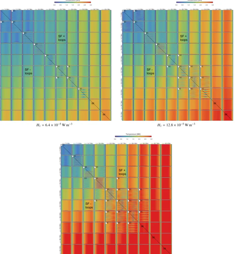
Figure 4.Temperature evolution for 300 loops from 1D hydrodynamic simulations using the loopA geometry (semicircular; see Figure2). Each grid plot shows a cut
through the heating parameter scan cube, i.e., each grid plot corresponds to a different value of H1(the heating imposed at the footpoints). λ1andλ2are scanned
between 2% and 11% of L, i.e., between 7.3 and 44.0Mm. The black dashed lines indicate the symmetric heating simulations (i.e., the diagonal of the squared grid plots for this loop geometry). Each small 2D plot shows the evolution of the temperature for one single simulation, along the loop (horizontal direction) and during the 72 hr of the simulation (vertical direction). The white dots indicate cases of TNE (see Section 2.3.2). For each TNE case we distinguish ICs (incomplete
condensations) from CCs (complete condensations). The approximated areas where the simulations are dominated by continuous siphon flows (surrounding the TNE area) are indicated by “SF+loops” and “SF − loops,” respectively, for left to right siphon flows and right to left ones. “SE” designates the loops in static equilibrium. The color scale is saturated at 3MK for every panel.
1. If it is a TNE case with a white dot, and either CC (for complete condensation) or IC (for incomplete condensation). CC cases can be visually identified by the dark-blue and purple drops in the temperature evolution (temperature 0.5 MK);
2. SF is stated for continuous siphonflows; 3. and SE for static equilibrium.
In order to determine whether a simulation exhibits TNE cycles and what the nature of the condensations are, we use the criteria presented in Section2.3.2. We see that TNE cycles are encountered only around the diagonal of each of these square grid plots, i.e., for simulations for which a symmetric heating function is applied. The upper limit for theses cycles is λ1=λ2=33.0 Mm (i.e., 9% of L), i.e., the solutions with
λ1orλ2larger than this value are stable. We also notice that the
more heating is applied(H1high, and consequently Q0high),
the more the TNE domain extends away from the diagonal. In Figure10, we show the maximum temperature and density averaged near the loop apex and the averaged velocity over the loop apex. This temperature is most of the time coronal(with very few simulations below∼0.6 MK). It increases to 4MK for large values of H1,λ1, andλ2. We see a clear signature of heating for
symmetric heating cases(with λ1∼λ2). Indeed, comparing with
Figure4, we can identify that within the TNE domain(indicated by the field of white dots in Figure 4), high temperatures are
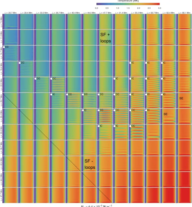
reached more easily. The maximum density plot shows also clearly a condensation pattern for the TNE simulations. We notice that this maximum density is up to ~10 m15 -3, which is a reasonable value for a large coronal loop(Reale2014). However, these values are Figure 5.Same as Figure4, but for the temperature evolution for 144 loops, using the loopB geometry (see Figure3). Parameter scan with H1=6.4×10⁻⁵ W m−3.λ1is
scanned between 7% and 18% of L, i.e., 25.7 and 66.1Mm, and λ2is scanned between 2% and 13% of L, i.e., between 7.3 and 47.7Mm. The black dashed line indicates the
symmetric heating simulations, which does not correspond to the diagonal of the grid plots for this loop geometry because the loop shape is not symmetric. The color scale is saturated at 3MK.
quite low for CC cases, but we have to bear in mind that we average these quantities around the apex before determining the maximum, and as we will see for other loop geometries, the density peak is not necessarily reached around the apex.
We notice that the velocity around the loop apex is quite high (~100 km s-1) when l +l < 40 Mm
1 2 , when the heating is
very stratified. The velocities are lower close to TNE cases. We use the velocity maps8 to analyze the loops without cycles. For each H1, in the region whereλ1>λ2, we encounter
loops whose evolution is dominated by siphon flows to the right footpoint (i.e., the less heated footpoint; see SF+ in Figure4). We witness the reversed siphon flows when λ1<λ2
(see SF− in Figure4). We have thus continuous siphon flows
to the less heated footpoint when the heating is strongly asymmetric. The last main behavior encountered is static equilibrium (velocity close to zero along the loop; see SE in Figure4), for the loops along the diagonal and with λ1,λ2>
33.0 Mm. Note that the TNE cases show periodic siphonflows (see Figure 16) but that the cases pointed out as SFs here are
simulations dominated by continuous siphonflows for several days. For each value of H1, the TNE, SF+, SF−, and SE
domains do not overlap.
To conclude for this semicircular loop geometry, we found that the majority of TNE cases produced CC cycles: between 82% and 89% of the TNE cases are CCs, depending on the H1
used. This is consistent with the results of Mikić et al. (2013; see, e.g., Case 7). A few ICs are encountered at the boundaries of the TNE domain(i.e., when the heating is asymmetric) when
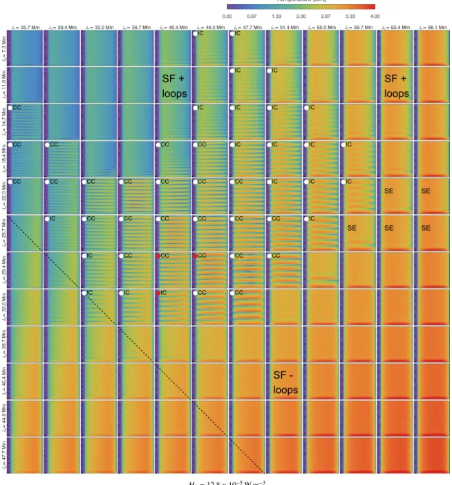
Figure 6.Same as Figure5, but withH1=12.8´10-5W m-3. The color scale is saturated at 4MK. The red dots indicate TNE cases studied in detail in Section4.1 and shown at higher resolution in Figure16.
8
We do not show the velocity maps in this paper for conciseness. However, Figure 10 allows us to identify the SE cases, without looking at the velocity maps.
the total heating is increasing(i.e., for higher H1). The domain
within the parameter space in which loops are undergoing TNE cycles is rather restricted to symmetric (or close to) heating cases. We notice that there is more dispersion around the diagonal when the total heating is increased.
2.3.4. Loop B
We use the same H0, i.e.,1 ´10-7W m-3, for the simulations
with this loop geometry. We scan two values9of H1: 640 H0, as
presented in Figure5, and 1280H0, as presented in Figure6. Note
that the temperature scale between these twofigures is different. It
will be the same for the plots concerning loopC. For each value of H1,λ1is scanned between 7% and 18% of L, i.e., we test 12
values between 25.7 and 66.1Mm, and λ2is scanned between 2%
and 13% of L, i.e., 12 values between 7.3 and 47.7Mm, for a total of 2×12×12=288 simulations.
The TNE cycles are also located in a restricted domain but are now shifted to the region whereλ1>λ2, i.e., asymmetric
heating cases when the eastern footpoint (leg) is heated more than the western one. Compared to loopA, the subfield of the parameter space presented here is thus not centered around the symmetric heating cases(indicated by the black dashed line). The scale heights for the energy deposition have to be larger than for loopA to reach TNE conditions.
Only one simulation shows TNE cycles with a symmetric heating function. For this simulation,λ1=λ2=33.0 Mm (for
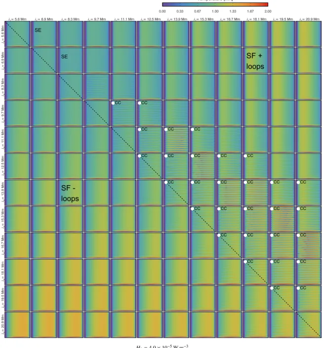
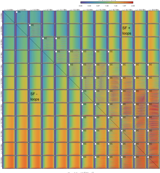
Figure 7.Same as Figure4, but for the temperature evolution for 144 loops, using the loopC geometry (see Figure3). Parameter scan withH1=4.0´10-5W m-3. λ1andλ2are scanned between 4% and 15% of L, i.e., between 5.6 and 20.9Mm. The black dashed line indicates the symmetric heating simulations (λ1=λ2), which
corresponds to the diagonal of the grid plots for this loop geometry. The color scale is saturated at 2MK.
9 In our analysis, we scanned a third value of H
1: 320H0; however, we
=
H1 1280H0; see Figure6). However, this simulation is at the edge of the TNE domain. The envelope of the TNE domain is roughly restricted to the following values: 1.0<λ1/λ2<3.4,
though the exact shape of the TNE domain is more complex. We notice that the range of λ1taken by TNE cases (between
7% and 17% of L) is wider than the one of λ2(between 2% and
9% of L). This is probably due to the asymmetry of the loop geometry, the field line from the LFFF extrapolations being skewed toward one footpoint.
As for loopA, the more the loop is heated, the wider the TNE domain is. Looking now at the condensations in these TNE cases for the two H1values scanned, we notice that 56% and 45% of
them, respectively, have cycles with ICs. Moreover, these IC cases tend to be at the edges of the TNE domain.
In the same way as for loopA, the maximum of the averaged apex temperature and density and the mean apex velocity are
displayed in Figure11. The values reached for both temperature and density are similar to the ones for loopA. We also see a larger apex temperature in the TNE domain, compared to the surrounding SF cases, as was the case for loopA. The velocities at the apex are much smaller than for loopA (maximum 15 km s−1). But we observe the same pattern of velocity evolution within the parameter space, i.e., higher velocities when the heating is highly stratified, λ1+λ2<60 Mm in that case. Moreover, as for loopA,
velocities at the apex are lower in the TNE domain.
At each side of the TNE domain, the simulations are dominated by siphon flows, the direction depending on the asymmetry of the heating. We also find a few SE cases (see location in Figures 5 and 6). Note that the white pixels in
Figure11do not necessarily indicate SE cases, as TNE cases can show zero velocities at the apex. SE cases point out no flows along the loop for most of the 3 days of the simulation.
Finally, it is worth noting the presence of high-frequency fluctuations (wavy pattern) in these simulations, especially around the eastern footpoint. We surmise that it is probably due to a combination of the thick chromosphere at this footpoint and the numerical treatment of the transition region. LoopB has a portion that is almost tangent to the photosphere at its eastern leg(i.e., with small projected gravity; see Figure3 and PaperI). Indeed, this sawtooth pattern is not observed for the
other loop geometries or for the high-resolution simulations in Figure16.
2.3.5. Loop C
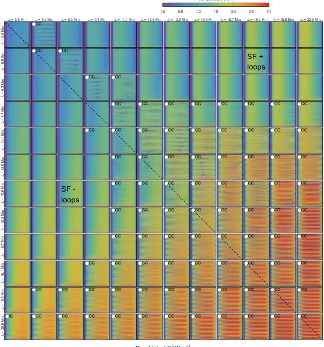
For this last loop geometry, we parameterize the heating function withH0=2´10-6W m-3. We scan three values of H1: 20H0, as presented in Figure 7, 40H0, as presented in
Figure8, and 80H0, as presented in Figure9. For each value of
H1, l1andλ2are scanned between 4% and 15% of L, i.e., we
test 12 values between 5.6 and 20.9Mm. Every combination is tested, so we have in total 3×12×12=432 simulations.
With this loop geometry, we notice that TNE cycles appear first for symmetric or slightly asymmetric heating conditions (λ1>λ2) whenH1=20H0. Then when we increase H1, more
TNE appears for asymmetric heating conditions, especially for λ1>λ2. Finally, whenH1=80H0, we can notice that the TNE domain becomes much larger than for loopsA and B. In particular, there does not appear to be a limit to TNE for large scale heights. However, the TNE domain remains limited, as barely any TNE cases appear for a very high stratification of the heating(λ1or λ2smaller than 8.3Mm).
We notice also that most of the TNE cases have CC cycles (0% of the TNE events for the first two values of H1and 1% for
the last one). The siphon flow cases surround the TNE domain,
with IC cycles starting to appear on the boundary of this domain.
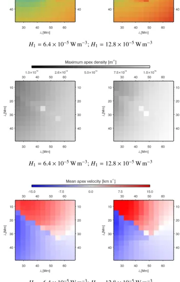
Figure 12 shows the maximum of the averaged apex temperature and density and the mean apex velocity. The temperature and density reached are similar to those of the other loops, but we clearly see the large range covered by the CC events (high temperature and high density). The velocities are close to the ones observed for loopB, but the pattern we observed for loopsA andB, i.e., higher velocities for small heating scale heights, is not as clear here.
3. The Occurrence of TNE
3.1. Conditions That Favor TNE and Constraints on the Heating
Scanning the parameter space of heating configurations for different loop geometries, we have noticed that the distribu-tion of the occurrence of TNE depends on the loop geometry. However, from this study, it seems that we are able to
produce TNE-favorable conditions for any loop geometry. TNE will occur if the heating strength is sufficient to produce a loop dense enough to create a thermal runaway at high altitudes, and if this heating is deposited on specific scale heights.
From the heating parameter-space scan that we conducted with three different loop geometries, we can conclude that a stratified heating is a necessary condition to produce TNE, but it is not sufficient, as already found by many authors (e.g., Müller2004; Susino et al.2010; Mikić et al.2013). For each
loop geometry, the system undergoes TNE cycles for specific heating stratifications:
1. l1l2 for loopA; 2. λ1>λ2for loopB;
3. for loopC, we observe two behaviors: λ1∼λ2when H1
is small,λ1or λ2>8.3 Mm when H1is large.
Figure 10. Evolution of the maximum temperature and density, and mean velocity around the loop apex within the heating parameter space(λ1,λ2, and
H1) for the simulations with the loopA geometry. Temperature and density are
averaged around the apex before determining the maximum. The velocity is displayed between 110 km s-1.
Figure 11. Same as Figure 10, but for the simulations using the loopB geometry. The velocity is displayed between 15 km s-1.
As stated before, in this paper we present only a subfield of the parameter space that we scanned. For each loop geometry, we also tested smaller and larger values of H1than the values
presented here. However, when H1 is too small, we do not
reach typical coronal loop temperatures and densities, and a large majority of the loops do not show any TNE cycles. When the H1are too large, the temperature of the loops is too high
(>4 MK) compared to the warm pulsating loops observed with AIA.
For all the loop geometries, the more heating (H1) is
applied at the footpoints, the less the system requires heating symmetry to achieve TNE cycles. In other words, higher H1
leads to more TNE within the parameter space. Higher H1
induces more chromospheric evaporation, which results in denser plasma at coronal altitudes, favoring the thermal runaway. Indeed, the input heating H1has to be sufficient to
inject the density required for triggering TNE events. The loops that we are modeling in this paper are quite large(367 and 139 Mm), and thus a large chromospheric evaporation is needed to inject enough density, which can explain the large Q0 values required to have TNE cycles (see values in
Table 1).
It is worth remembering that the loopC geometry is extracted from afield line corresponding to a loop bundle that is not undergoing cycles in the observations. Interestingly, it is for this loop geometry that the TNE cycles have the highest probability10to occur, according to our simulation results with the highest H1 tested. If our model (quasi-steady stratified
heating) is indeed correct, it would mean that we can constrain the heating for these particular loops. That would mean that loopC, which is not showing any pulsations in the AIA data, is not heated enough at the footpoints to inject the excess of density needed in the loop bundle to trigger the thermal runaway, and/or that the heating is very stratified. In the same way, loopB is showing pulsations in the AIA data, so we can guess that for this loop bundle the heating is asymmetric, stratified, and relatively important.
3.2. Exploration De-correlated from the Magnetic Field Strength
For each of the geometries tested, not all the stratified heating configurations lead to TNE. The area where TNE occurs is limited to some range in the heating parameter space. This leads to the question as to whether the area explored within the parameter space is realistic. In particular, the heating is somewhat correlated to the magneticfield strength (see, e.g., turbulent models in Rappazzo et al. 2007), and therefore we
may have explored heating parameters that are unrealistic. On the other hand, the strength of the magneticfield along the loops does not take into account the magnetic topology, which necessarily influences the heating as well (formation of separatrices, preferential reconnection sites; e.g., Aly & Amari 1997; Pariat et al. 2009; Parnell et al. 2010; Wyper et al. 2012). The heating parameter-space scan for loopB
shows that we can produce TNE cycles for this loop geometry only with asymmetric heating profiles. This heating configura-tion was validated a posteriori in PaperI by the magnetic topology found around the eastern footpoints of this loop bundle, which can favor continuous reconnection and thus enhanced heating.
3.3. Common Characteristics of TNE Events
From the analysis of the flows, using in particular the averaged apex velocity (see Section2.3), we noticed that the
siphonflows are more intense for short heating scale heights. Moreover, they tend to be weaker close to the TNE conditions (see Figures13–15).
We examine also some characteristics of the cycles of the TNE cases. Figures 13–15 show, for each simulation, the periods of the cycles and time lags between the temperature and density averaged around the apex.
Period of the TNE cycles—We can notice an evident dependence on the loop length. The periods are from 2.5 to 15.5hr for loopA, and from 5.5 to 15.5hr loopB, which are both 367Mm long, and from 2.4 to 5.9hr for loopC, which is 139Mm long. This dependence has already been seen in the EIT event statistics of Auchère et al. (2014), the AIA event
statistics of Froment (2016), and the three events of Froment
et al. (2015). For loopA, the period of the cycles increases
along the diagonal of each H1-constant grid and between two
grids, i.e., when Q0, and thus the maximum Teat the apex, is
Figure 12. Same as Figure 10, but for the simulations using the loopC geometry. The velocity is displayed between 15 km s-1.
10
increasing. For the other loops, we find the same general dependence, but the detailed behavior is more complex. The period increases with Q0andL.
Time lag between Te and ne—We compute the time lag
between the temperature and density evolution. This delay is also a characteristic of TNE cycles; it is a signature of TNE when combined with the periodicity. It also explains the systematic cooling pattern observed between EUV channels, the intensity peakingfirst in the hotter channels and then in the cooler ones (e.g., Viall & Klimchuk 2012). In case of TNE
events this observed cooling can be explained by a faster rise of the temperature than the temperature fall combined with, or only if, the density is low during the heating phase compared to the cooling phase(see Section 3.2.3 in PaperIfor more details). This time lag is given here by the peak of the cross-correlation between the average temperature and density curves around the loop apex. We choose to display them as a fraction of the period in order to compare the cases more easily. We explore systematically positive time delays between 0% and 60% of the TNE cycle period. Indeed, to our knowledge, no TNE simulations have been reported to show an increasing of the density before the temperature and the signal being periodic
we avoid in that way to detected spurious negative time lags between Teand ne. For loopA, we notice that there are very
long delays when there are very strong CCs. In some cases this delay is close to the period (see the notes in Table 1).
Moreover, for some CC cases the shapes of the temperature and density curves are very different, which leads to poor cross-correlation values and underestimated time lags (not catching the strongest density peak). For loopsBandC the time lags tend to be maximum close to symmetric heating cases, otherwise becoming quite uniform within the TNE domain, i.e., about 20%–30% of the period, which is what was observed in Froment et al.(2015).
4. Loop Behaviors in These Simulations and Comparison with the Observations
4.1. EUV Pulsations and Coronal Rain
Figure16shows three TNE cases for loopB. We display the temperature, density, and velocity evolution along the loop, for 3 days of simulation, i.e., about eight evaporation/ condensation cycles (giving thus a period close to the one detected for event 1 in Froment et al.2015). These simulations Figure 13.Evolution of different properties of the TNE cases within the heating parameter space(λ1,λ2, and H1) for the simulations with the loopA geometry. The
black areas designate simulations where we do not detect TNE cycles. Top: period of the TNE cycles. Bottom: time lag between Teand nearound the loop apex,
are extracted from Figure 6 and thus correspond to H1=
´ -
-12.8 10 5W m 3. They are indicated by a red dot in Figure 6. They all have similar heating conditions. However, and as discussed earlier, these simulations are repeated using the unmodified Spitzer conductivity and 100,000 mesh points, as in PaperI.
The first simulation is an IC case for which λ1=40.4 Mm
andλ2=33.0 Mm. Note that this simulation is not the same as
the one presented in PaperI (with λ1=50 Mm and
λ2=20 Mm) that has the same loop geometry. The two other
simulations present CCs, with different locations of the condensations. For the middle simulation, λ1=44.0 Mm and
λ2=29.4 Mm, and the condensations form close to the apex.
For the last simulation,λ1=40.4 Mm and λ2=29.4 Mm, and
the condensations form closer to the eastern footpoint. At t1, we
display the loop profiles when the temperature reaches a maximum at the apex for one of the cycles, and at t2the profiles
when the temperature reaches a local minimum. These three loops have a maximum apex temperature around 3MK. During the cooling phase, when the condensations are established, the temperature drops to ∼1MK in the eastern leg of the IC simulation, while the density increases by a factor of ∼2. For the CC simulations, the temperature drops locally to 0.01MK and the density increases by a factor of 10.
We also notice a larger velocity for CC (up to 140 km s−1) compared to the IC case (about 10 km s−1 at the footpoints), probably due to the increase of the density of the condensation that falls compared to the density of the loop itself. The velocity is also higher when the CC starts closer to the apex, due to the longer acceleration time. We notice periodic siphon flows for both the IC and the CC cases, the ones for CCs being stronger.
As already indicated before, around the apex, the amplitudes of the temperature (and even the density) evolution are not dramatically different for the complete and incomplete cases. The CC, which is triggered in the eastern leg, outside of the apex area, has a minimal effect on the temperature evolution around the apex. It is thus not possible to use the evolution of the parameters at the apex to distinguish between complete and incomplete cases.
In Figure17, we trace the evolution of the EUV intensity as it would have been seen in the 171, 193, and 335Åchannels of AIA(see Section 3.2.1 of PaperIfor computation details), for these three loop systems(noted as IC, CC 1, and CC 2). As in PaperI, we used the AIA response functions to isothermal plasma for each channel, calculated with CHIANTI version 8.0 (Del Zanna et al.2015). For comparison, we add the same plot
from the AIA observations. The intensity is given along the loop defined by a smoothed version of the orange contour11 displayed in Figure 1. However, as we already pointed out in detail in PaperI, the synthetic intensity can only be examined in the coronal part of the loop (due to the limitations of the model, we exclude the chromosphere and the low-transition region of the intensity analysis). We will discuss in more detail the intensity variation and values along the observed contour in the next section.
The overall pulsating behavior is well reproduced in the three simulations. In both complete and incomplete cases we can find the same global cooling pattern, with the intensity peakingfirst at 335 Å, then 193 Å, and finally 171 Å, following the order of the peak responses of the channels. Note that we choose these three simulations because they show condensa-tions to the eastern footpoint and thus match the intensity pattern(higher intensities close to the eastern footpoint) along the observed loop bundle. The simulation presented in PaperI
showed condensations to the western leg of the loop. This heating case showed the most convincing intensity light curves at the apex (and directly comparable to the observed light curves) among the simulations of the parameter space explored. However, the IC case chosen in the present paper shows a more convincing pattern along the loop for the reason detailed above (asymmetry of the intensity between the two loop legs).
Between the IC and CC simulations, the biggest differ-ences12 occur at the location of the triggering of the condensations, where we can see another 335 Å peak, corresponding to the 0.2MK peak of that band.13 However, it seems quite challenging to look for this smaller peak in AIA data, as it is probably hidden in the line-of-sight integration to distinguish between CC and IC cases.
The pulsations that we observed in Froment et al. (2015)
may also include co-spatial and simultaneous coronal rain events. However, it is quite difficult to distinguish between complete and incomplete cases using only the coronal channel of AIA, as discussed in Froment et al.(2017). It also remains
difficult to conclude firmly for on-disk observations. However,
Figure 14. Same as Figure 13, but for the simulations using the loopB geometry.
11
Note that the length of the observed loop is then a bit shorter than the length of the simulated loops(derived from LFFF extrapolations). It does not affect our analysis, as we discard the synthetic intensities from the simulated footpoints.
12
We notice also smaller intensity values for the cooling phases of the CCs cases than for the ones of the IC case, but with only one loop it can be delicate to focus on absolute values.
13
The peak at lower temperature(OIIIto OVlines) has been accounted for in the AIA response function since February 2013(version 4), following the measurement of Soufli et al. (2012).
the time lag between the 171 Å and 131 Å channels can help to identify the nature of the condensations even if we only have access to the mean behavior of the loop bundles. In Auchère et al. (2018), the authors detect long-period EUV pulsations
coincident with coronal rain, in a region observed off-limb. In this study the 131 Å intensity peaks after 171 Å, which was not the case for the events studied on-disk in Froment et al.(2015).
We found no time lag between these channels, which indicates that the temperature of the plasma did not decrease on average below the peak response of 171(around 0.8 MK).
4.2. Are All the Results of These Simulations Realistic? We have previously seen that some of the TNE cases can reproduce very well the average behavior observed with AIA, in the case of long-period intensity pulsations (see also the results of PaperI). Looking beyond the TNE cases, we can ask
ourselves whether the non-TNE cases produced in the parameter space are realistic. Only a few simulations are hydrostatic, and most of the non-TNE simulations are dominated by continuous siphon flows lasting for most of the 3 days of the simulations. For these cases the simulated intensity would not show any temporal variations, which is inconsistent with observed EUV loops. In this regard, we have to bear in mind that in this simplified analysis we have
modeled the average behavior of loop systems and have not included the variability of the heating that is likely to occur in the corona. Further studies, including an exploration of the temporal variations of the heating and/or loop geometry, are needed to quantify the dynamics of these systems and their stability.
One way to check whether the densities produced by our simulations are consistent with observations is to compare the observed AIA intensities with the simulated ones. In Figure17, we display the intensity along loopB for three different simulations, as it would be seen with AIA, considering a radius of the cross section of the loop bundle of 100km at s=0. The intensity values in DN s−1 are between 0.1 and 10, except during the cooling phases. Considering that the loop intensity is about 10% above the background emission (Del Zanna & Mason 2003; Viall & Klimchuk 2011), this is consistent with
the intensity counts derived from AIA observations (between about 1 and 100 DN s−1) displayed in the same figure. The fact that we model only one loop also explains why we can easily identify the condensations in the profiles. In contrast, in the AIA observations the difference of intensity between the heating and cooling phase profiles chosen at t1and t2is quite
small. The signature of the condensations is probably hidden by the background and foreground emission.
Figure 16.Evolution of the temperature Te, density ne, and longitudinal velocity v for three simulations using the loopB geometry. These simulations use the same
heating parameters as the simulations indicated by red dots in Figure6( =H1 12.8´10-5W m-3). They are repeated here using the classic Spitzer conductivity and 100,000 mesh points. First column: incomplete condensation simulation (IC), with λ1=40.4 Mm and λ2=33.0 Mm. Second column: complete condensation
simulation withλ1=44.0 Mm and λ2=29.4 Mm (CC 1). Third column: complete condensation simulation with λ1=40.4 Mm and λ2=29.4 Mm (CC 2). Each
line represents respectively the evolution of Te, ne, and v along the loop during the 72 hr of the simulation(in the style of Figure 4 of PaperI). On the right of the 2D
plots, we display the evolution of respectively Te, ne, and v around the loop apex(mean value between the two dotted bars in the bottom panel). On the bottom of the
2D plots, we show two profiles (solid and dashed lines, corresponding respectively to the hot phase at t1and the cool phase at t2, indicated by the solid and dashed
lines in the right panels). Note that t1and t2are different for each simulation. For the velocity, red(positive) is for flows from the eastern footpoint to the western one,
Figure 17.Comparison between the synthetic AIA intensities for the IC and CC simulations presented in Figure16and the observed intensity evolution along the pulsating loop bundle. The 171Åchannel is plotted in red, 193 Åin green, and 335 Åin blue. The average intensities, normalized to variance, are plotted on the right of each 2D plot. The t1and t2profiles are plotted under each 2D plot, in the same way as in Figure16. The black area in the 2D plots and the gray hashed regions on
the loop profiles, i.e., the parts of the loop under s=70Mm and above s=350Mm, are not considered, as the simulations and the intensity calculation are only correct in the coronal part of the loop(see Section 3.2.2. in PaperI). The actual AIA intensities are extracted from a smoothed version of the orange contour of
Figure1. We also trace the evolution of the intensity in a portion around the loop apex(looking at the profiles along the contour), and the intensity profiles in the same way as for the simulations. Note that the range of intensities displayed is not the same as for the profiles from the simulations.
5. Summary
In this paper, we explored a large range of dynamics, scanning different regimes of thermal nonequilibrium (TNE) and other behaviors in coronal loops. Several parameter-space studies regarding TNE cycles have already been conducted (e.g., Müller2004; Susino et al.2010; Mikić et al.2013). Our
study takes into account the recent discovery that long-period intensity pulsations are commonly observed in coronal loops.
The 1D hydrodynamic description of loops we used allows us to rapidly scan the parameter space. The model presented is rather simple but captures the highly nonlinear dynamics of coronal loops. Indeed, we are able to nicely summarize the thermo-dynamic evolution of loops, even though the transition region and chromospheric behavior cannot be examined in detail.
For this extensive study we chose to explore a broad range of heating configurations, without explicitly limiting the heating profiles to a function of the magnetic field strength. We present in this paper a subset of this study, showing the results of 1020 simulations.
We found TNE events in specific regions of the parameter space explored. With the different loop geometries (one semicircular and two from LFFF extrapolations) used for the heating parameter scan, we conclude the following:
1. Any loop geometry seems suitable for a loop system to undergo TNE cycles.
2. However, for each loop geometry the heating require-ments to obtain TNE cycles are not the same.
3. A stratified heating is a necessary condition, but it is not sufficient to produce TNE. For each loop geometry, the heating parameter domain where we obtain TNE is different.
4. The domain where wefind TNE in the heating parameter space is limited.
5. The more the heating is important at the footpoints, the more the loop is likely to undergo TNE cycles and in particular complete condensations (CCs), rather than incomplete condensations (ICs), due to the high density of the plasma injected in the loop from chromospheric evaporations.
These conclusions might at first sight imply that any loop system could undergo condensation and evaporation cycles. However, this is not the case. In reality, the geometry and heating conditions vary from point to point. For a given loop, only one set of heating parameters exists. TNE is only possible when there is a specific match between the loop geometry and the heating conditions.
Indeed, the long-period intensity pulsations reported by Auchère et al.(2014) and identified as TNE cycles by Froment
et al.(2015,2017) are widely observed in the corona but not in
every loop bundle. There are probably many more cases of such cycles in loops, with heating conditions that change too much over time, producing more limited and irregular cycles. The Auchère et al. (2014) technique was designed to detect
regular intensity pulsations and is thus most sensitive to TNE events with stable pulsations. The detection of the probably more frequent cases in which coronal conditions evolve with time would require a different method.
Our work presents several limitations, in particular, simple input heating, poor treatment in the chromosphere and the transition region, simulation of a single loop, and no time dependence of the heating. However, it aims to be a first step
toward the exploration of the complex parameter space we only merely touched on. More parameters could play an important role in triggering and maintaining evaporation and condensation cycles. Eventually, elaborate simulations, possibly multidimen-sional, with a proper forward modeling could help to constrain the heating of the loop observed by comparing their behavior (cycles or not, period, time lag between the temperature and the density evolution, etc.) with the results of such simulations.
This extensive parameter-space study also allowed us to explore some characteristics of the TNE events. These characteristics are summarized in Table 1 and Figures 13–15. We found that the period(from 2.4 to 15.5 hr) is increasing with the length of the loop and with the maximum temperature reached. These periods also tend to be longer for CC compared to IC for the same loop geometry. The time delay between the temperature and density evolution, characteristic of TNE events when combined with the periodicity, is constant to within 20%–30% of the period for most of the simulations (strong CC cases are an exception). We found also that some loop geometries are more favorable to CC cases (see loop C). Moreover, looking at IC and CC cases in more detail, we show that both are exhibiting siphonflows during the cooling phases. For CCs theseflows are stronger. This is consistent with 2.5D magnetohydrodynamic simulations of Fang et al.(2013,2015).
To conclude, we presented a unified picture of numerical simulations of cooling/heating in loops. We reaffirm in particular that coronal rain and long-period intensity pulsations are two manifestations of the same phenomenon, as demonstrated observationally by Auchère et al.(2018).
This work is an outgrowth of the work presented during the VII Coronal Loop Workshop and at Hinode 9. The authors acknowledge useful comments from attendees of these conferences. The authors would like to thank Jim Klimchuk and Patrick Antolin for fruitful discussions on thermal nonequilibrium and long-period pulsations in loops. The SDO/AIA and SDO/HMI data are available courtesy of NASA/SDO and the AIA and HMI science teams. This work used data provided by the MEDOC data and operations center (CNES/CNRS/Univ. Paris-Sud),http://medoc.ias.u-psud.fr/. Z.M. was supported by NASA Heliophysics Supporting Research grant NNX16AH03G. This research was supported by the Research Council of Norway, project no. 250810, and through its Centres of Excellence scheme, project no. 262622.
ORCID iDs C. Froment https://orcid.org/0000-0001-5315-2890 F. Auchère https://orcid.org/0000-0003-0972-7022 Z. Mikić https://orcid.org/0000-0002-3164-930X G. Aulanier https://orcid.org/0000-0001-5810-1566 K. Bocchialini https://orcid.org/0000-0001-9426-8558 E. Buchlin https://orcid.org/0000-0003-4290-1897 E. Soubrié https://orcid.org/0000-0001-9295-1863 References
Aly, J. J., & Amari, T. 1997, A&A,319, 699
Antiochos, S. K., & Klimchuk, J. A. 1991,ApJ,378, 372
Antiochos, S. K., MacNeice, P. J., & Spicer, D. S. 2000,ApJ,536, 494
Antiochos, S. K., MacNeice, P. J., Spicer, D. S., & Klimchuk, J. A. 1999,ApJ,
512, 985
Antolin, P., & Rouppe van der Voort, L. 2012,ApJ,745, 152
Antolin, P., Vissers, G., Pereira, T. M. D., Voort, L. R. v. d., & Scullion, E. 2015,ApJ,806, 81
Antolin, P., Vissers, G., & Rouppe van der Voort, L. 2012,SoPh,280, 457
Auchère, F., Bocchialini, K., Solomon, J., & Tison, E. 2014,A&A,563, A8
Auchère, F., Froment, C., Bocchialini, K., Buchlin, E., & Solomon, J. 2016a,
ApJ,825, 110
Auchère, F., Froment, C., Bocchialini, K., Buchlin, E., & Solomon, J. 2016b,
ApJ,827, 152
Auchère, F., Froment, C., Soubrié, E., et al. 2018,ApJ,853, 176
Boerner, P., Edwards, C., Lemen, J., et al. 2012,SoPh,275, 41
De Groof, A., Bastiaensen, C., Müller, D. A. N., Berghmans, D., & Poedts, S. 2005,A&A,443, 319
De Groof, A., Berghmans, D., van Driel-Gesztelyi, L., & Poedts, S. 2004,
A&A,415, 1141
Delaboudinière, J.-P., Artzner, G. E., Brunaud, J., et al. 1995, SoPh,162, 291
Del Zanna, G., Dere, K. P., Young, P. R., Landi, E., & Mason, H. E. 2015,
A&A,582, A56
Del Zanna, G., & Mason, H. E. 2003,A&A,406, 1089
Domingo, V., Fleck, B., & Poland, A. I. 1995,SoPh,162, 1
Fang, X., Xia, C., & Keppens, R. 2013,ApJL,771, L29
Fang, X., Xia, C., Keppens, R., & Van Doorsselaere, T. 2015,ApJ,807, 142
Froment, C. 2016, PhD thesis, Université Paris-Saclay, Université Paris-Sud, Institut d’Astrophysique Spatiale
Froment, C., Auchère, F., Aulanier, G., et al. 2017,ApJ,835, 272
Froment, C., Auchère, F., Bocchialini, K., et al. 2015,ApJ,807, 158
Guennou, C., Auchère, F., Klimchuk, J. A., Bocchialini, K., & Parenti, S. 2013,
ApJ,774, 31
Guennou, C., Auchère, F., Soubrié, E., et al. 2012a,ApJS,203, 25
Guennou, C., Auchère, F., Soubrié, E., et al. 2012b,ApJS,203, 26
Karpen, J. T., & Antiochos, S. K. 2008,ApJ,676, 658
Karpen, J. T., Antiochos, S. K., & Klimchuk, J. A. 2006,ApJ,637, 531
Klimchuk, J. A., Karpen, J. T., & Antiochos, S. K. 2010,ApJ,714, 1239
Kuin, N. P. M., & Martens, P. C. H. 1982, A&A,108, L1
Lemen, J. R., Title, A. M., Akin, D. J., et al. 2012,SoPh,275, 17
Lionello, R., Alexander, C. E., Winebarger, A. R., Linker, J. A., & Mikić, Z. 2016,ApJ,818, 129
Lionello, R., Linker, J. A., & Mikić, Z. 2009,ApJ,690, 902
Lionello, R., Winebarger, A. R., Mok, Y., Linker, J. A., & Mikić, Z. 2013,
ApJ,773, 134
Mendoza-Briceño, C. A., Sigalotti, L. D. G., & Erdélyi, R. 2005,ApJ,624, 1080
Mikić, Z., Lionello, R., Mok, Y., Linker, J. A., & Winebarger, A. R. 2013,
ApJ,773, 94
Mok, Y., Mikić, Z., Lionello, R., Downs, C., & Linker, J. A. 2016,ApJ,817, 15
Mok, Y., Mikić, Z., Lionello, R., & Linker, J. A. 2008,ApJL,679, L161
Müller, D. A. N. 2004, PhD thesis, Kiepenheuer Institute for Solar Physics, Freiburg and Institute of Theoretical Astrophysics, Oslo
Müller, D. A. N., De Groof, A., Hansteen, V. H., & Peter, H. 2005,A&A,
436, 1067
Müller, D. A. N., Hansteen, V. H., & Peter, H. 2003,A&A,411, 605
Müller, D. A. N., Peter, H., & Hansteen, V. H. 2004,A&A,424, 289
Pariat, E., Masson, S., & Aulanier, G. 2009,ApJ,701, 1911
Parnell, C. E., Haynes, A. L., & Galsgaard, K. 2010,JGRA,115, A02102
Pesnell, W. D., Thompson, B. J., & Chamberlin, P. C. 2012,SoPh,275, 3
Rappazzo, A. F., Velli, M., Einaudi, G., & Dahlburg, R. B. 2007, ApJL,
657, L47
Reale, F. 2014,LRSP,11, 4
Scherrer, P. H., Schou, J., Bush, R. I., et al. 2012,SoPh,275, 207
Schrijver, C. J. 2001,SoPh,198, 325
Soufli, R., Spiller, E., Windt, D. L., et al. 2012,Proc. SPIE,8443, 84433C
Susino, R., Lanzafame, A. C., Lanza, A. F., & Spadaro, D. 2010,ApJ,709, 499
Vashalomidze, Z., Kukhianidze, V., Zaqarashvili, T. V., et al. 2015,A&A,
577, A136
Viall, N. M., & Klimchuk, J. A. 2011,ApJ,738, 24
Viall, N. M., & Klimchuk, J. A. 2012,ApJ,753, 35
Winebarger, A. R., Lionello, R., Mok, Y., Linker, J. A., & Mikić, Z. 2014,
ApJ,795, 138
Wyper, P. F., Jain, R., & Pontin, D. I. 2012,A&A,545, A78
Xia, C., Chen, P. F., Keppens, R., & van Marle, A. J. 2011,ApJ,737, 27